A Spectral Method for the Eigenvalue Problem for Elliptic Equations

Kendall Atkinson Affiliation: Departments of Mathematics & Computer Science Affiliation: The University of Iowa Olaf Hansen Affiliation: Department of Mathematics Affiliation: California State University San Marcos

Abstract

Let $\Omega$ be an open, simply connected, and bounded region in $\mathbb{R}^{d}$ , $d\geq 2$ , and assume its boundary $\partial\Omega$ is smooth. Consider solving the eigenvalue problem $Lu=\lambda u$ for an elliptic partial differential operator $L$ over $\Omega$ with zero values for either Dirichlet or Neumann boundary conditions. We propose, analyze, and illustrate a ‘spectral method’ for solving numerically such an eigenvalue problem. This is an extension of the methods presented earlier in [5], [6].

1 INTRODUCTION

We consider the numerical solution of the eigenvalue problem

Lu(s)\equiv-\sum_{k,\ell=1}^{d}\frac{\partial}{\partial s_{k}}\left(a_{k,\ell}(s)\frac{\partial u(s)}{\partial s_{\ell}}\right)+\gamma(s)u(s)=\lambda u(s),\quad\quad s\in\Omega\subseteq\mathbb{R}^{d}

(1)

with the Dirichlet boundary condition

u(s)\equiv 0,\quad\quad s\in\partial\Omega.

(2)

Assume $d\geq 2$ . Let $\Omega$ be an open, simply–connected, and bounded region in $\mathbb{R}^{d}$ , and assume that its boundary $\partial\Omega$ is smooth and sufficiently differentiable. Similarly, assume the functions $\gamma(s)$ and $a_{i,j}(s)$ , $1\leq i,j\leq d$ , are several times continuously differentiable over $\overline{\Omega}$ . As usual, assume the matrix $A(s)=\left[a_{i,j}(s)\right]$ is symmetric and satisfies the strong ellipticity condition,

\xi^{\text{T}}A(s)\xi\geq c_{0}\xi^{\text{T}}\xi,\quad\quad s\in\overline{\Omega},\quad\xi\in\mathbb{R}^{d}

(3)

with $c_{0}>0$ . For convenience and without loss of generality, we assume $\gamma(s)\geq 0$ , $s\in\Omega$ ; for otherwise, we can add a multiple of $u(s)$ to both sides of (1), shifting the eigenvalues by a known constant.

In the earlier papers [5] and [6] we introduced a spectral method for the numerical solution of elliptic problems over $\Omega$ with Dirichlet and Neumann boundary conditions, respectively. In the present work, this spectral method is extended to the numerical solution of the eigenvalue problem for (1)–(2), and in a later section it is also extended to the Neumann problem

	$\displaystyle-\Delta u(s)$	$\displaystyle=\lambda u(s),\quad\quad s\in\Omega\vskip 3.0pt plus 1.0pt minus 1.0pt$
	$\displaystyle\frac{\partial u}{\partial n}$	$\displaystyle=0,\quad\quad s\in\partial\Omega.$

2 The Dirichlet problem

Our spectral method is based on polynomial approximation on the unit ball $B_{d}$ in $\mathbb{R}^{d}$ . To transform a problem defined on $\Omega$ to an equivalent problem defined on $B_{d}$ , we review some ideas from [5] and [6], modifying them as appropriate for this paper.

Assume the existence of a function

\Phi:\overline{B}_{d}\underset{onto}{\overset{1-1}{\longrightarrow}}\overline{\Omega}

(4)

with $\Phi$ a twice–differentiable mapping, and let $\Psi=\Phi^{-1}:\overline{\Omega}\underset{onto}{\overset{1-1}{\longrightarrow}}\overline{B}_{d}$ . For $v\in L^{2}\left(\Omega\right)$ , let

\widetilde{v}(x)=v\left(\Phi\left(x\right)\right),\quad\quad x\in\overline{B}_{d}\subseteq\mathbb{R}^{d}

(5)

and conversely,

v(s)=\widetilde{v}\left(\Psi\left(s\right)\right),\quad\quad s\in\overline{\Omega}\subseteq\mathbb{R}^{d}.

(6)

Assuming $v\in H^{1}\left(\Omega\right)$ , we can show

\nabla_{x}\widetilde{v}\left(x\right)=J\left(x\right)^{\text{T}}\nabla_{s}v\left(s\right),\quad\quad s=\Phi\left(x\right)

with $J\left(x\right)$ the Jacobian matrix for $\Phi$ over the unit ball $B_{d}$ ,

J(x)\equiv\left(D\Phi\right)(x)=\left[\frac{\partial\varphi_{i}(x)}{\partial x_{j}}\right]_{i,j=1}^{d},\quad\quad x\in\overline{B}_{d}.

(7)

To use our method for problems over a region $\Omega$ , it is necessary to know explicitly the functions $\Phi$ and $J$ . We assume

\det J(x)\neq 0,\quad\quad x\in\overline{B}_{d}.

(8)

Similarly,

\nabla_{s}v(s)=K(s)^{\text{T}}\nabla_{x}\widetilde{v}(x),\quad\quad x=\Psi(s)

with $K(s)$ the Jacobian matrix for $\Psi$ over $\Omega$ . By differentiating the identity

\Psi\left(\Phi\left(x\right)\right)=x,\quad\quad x\in\overline{B}_{d}

we obtain

K\left(\Phi\left(x\right)\right)=J\left(x\right)^{-1}.

(9)

Assumptions about the differentiability of $\widetilde{v}\left(x\right)$ can be related back to assumptions on the differentiability of $v(s)$ and $\Phi(x)$ .

Lemma 1

If $\Phi\in C^{k}\left(\overline{B}_{d}\right)$ and $v\in C^{m}\left(\overline{\Omega}\right)$ , then $\widetilde{v}\in C^{q}\left(\overline{B}_{d}\right)$ with $q=\min\left\{k,m\right\}$ .

Proof. A proof is straightforward using (5).

A converse statement can be made as regards $\widetilde{v}$ , $v$ , and $\Psi$ in (6).

Consider now the nonhomogeneous problem $Lu=f$ ,

Lu(s)\equiv-\sum_{k,\ell=1}^{d}\frac{\partial}{\partial s_{k}}\left(a_{k,\ell}(s)\frac{\partial u(s)}{\partial s_{\ell}}\right)+\gamma(s)u(s)=f(s),\quad\quad s\in\Omega\subseteq\mathbb{R}^{d}.

(10)

Using the transformation (4), it is shown in [5, Thm 2] that (10) is equivalent to

\begin{array}[c]{r}-{\displaystyle\sum\limits_{k,\ell=1}^{d}}\dfrac{\partial}{\partial x_{k}}\left(\widetilde{a}_{k,\ell}(x)\det\left(J(x)\right)\dfrac{\partial\widetilde{v}(x)}{\partial x_{\ell}}\right)+\left[\widetilde{\gamma}(x)\det J(x)\right]\,\widetilde{u}(x)\\ =\widetilde{f}\left(x\right)\det J(x),\quad\quad x\in B_{d}\end{array}

(11)

with the matrix $\widetilde{A}\left(x\right)\equiv\left[\widetilde{a}_{i,j}(x)\right]$ given by

\widetilde{A}\left(x\right)=J\left(x\right)^{-1}A\left(\Phi\left(x\right)\right)J\left(x\right)^{-\text{T}}.

(12)

The matrix $\widetilde{A}$ satisfies the analogue of (3), but over $B_{d}$ . Thus the original eigenvalue problem (1)–(2) can be replaced by

\begin{array}[c]{r}-{\displaystyle\sum\limits_{k,\ell=1}^{d}}\dfrac{\partial}{\partial x_{k}}\left(\widetilde{a}_{k,\ell}(x)\det\left(J(x)\right)\dfrac{\partial\widetilde{u}(x)}{\partial x_{\ell}}\right)+\left[\widetilde{\gamma}(x)\det J(x)\right]\,\widetilde{u}(x)\\ =\lambda\widetilde{u}(x)\det J(x),\quad\quad x\in B_{d}\end{array}

(13)

As a consequence of this transformation, we can work with an elliptic problem defined over $B_{d}$ rather than over the original region $\Omega$ .

2.1 The variational framework

To develop our numerical method, we need a variational framework for (10) with the Dirichlet condition $u=0$ on $\partial\Omega$ . As usual, multiply both sides of (10) by an arbitary $v\in H_{0}^{1}\left(\Omega\right)$ , integrate over $\Omega$ , and apply integration by parts. This yields the problem of finding $u\in H_{0}^{1}\left(\Omega\right)$ such that

\mathcal{A}\left(u,v\right)=\left(f,v\right)\equiv\ell\left(v\right),\quad\quad\text{for all }v\in H_{0}^{1}\left(\Omega\right)

(14)

with

\mathcal{A}\left(v,w\right)=\int_{\Omega}\left[\sum_{k,\ell=1}^{d}a_{k,\ell}(s)\frac{\partial v(s)}{\partial s_{\ell}}\frac{\partial w(s)}{\partial s_{k}}+\gamma(s)v(s)w(s)\right]ds,\quad v,w\in H_{0}^{1}\left(\Omega\right).

(15)

The right side of (14) uses the inner product $\left(\cdot,\cdot\right)$ of $L^{2}\left(\Omega\right)$ . The operators $L$ and $\mathcal{A}$ are related by

\left(Lu,v\right)=\mathcal{A}\left(u,v\right),\quad\quad u\in H^{2}\left(\Omega\right),\quad v\in H_{0}^{1}\left(\Omega\right),

(16)

an identity we use later. The function $\mathcal{A}$ is an inner product and it satisfies

\left|\mathcal{A}\left(v,w\right)\right|\leq c_{\mathcal{A}}\left\|v\right\|_{1}\left\|w\right\|_{1},\quad\quad v,w\in H_{0}^{1}\left(\Omega\right)

(17)

\mathcal{A}\left(v,v\right)\geq c_{e}\|v\|_{1}^{2},\quad\quad v\in H_{0}^{1}\left(\Omega\right)

(18)

for some positive constants $c_{\mathcal{A}}$ and $c_{e}$ .

Associated with the Dirichlet problem

	$\displaystyle Lu(x)$	$\displaystyle=f(x),\quad\quad x\in\Omega,\quad f\in L^{2}\left(\Omega\right)$		(19)
	$\displaystyle u(x)$	$\displaystyle=0,\quad\quad x\in\partial\Omega$		(20)

is the Green’s function integral operator

u(x)=\mathcal{G}f(x).

(21)

Lemma 2

The operator $\mathcal{G}$ is a bounded and self–adjoint operator from $L^{2}\left(\Omega\right)$ into $H_{0}^{2}\left(\Omega\right)$ . Moreover, it is a compact operator from $L^{2}\left(\Omega\right)$ into $H_{0}^{1}\left(\Omega\right)$ , and more particularly, it is a compact operator from $H_{0}^{1}\left(\Omega\right)$ into $H_{0}^{1}\left(\Omega\right)$ .

Proof. A proof can be based on [16, §6.3, Thm. 5] together with the fact that the embedding of $H_{0}^{2}\left(\Omega\right)$ into $H_{0}^{1}\left(\Omega\right)$ is compact. The symmetry follows from the self–adjointness of the original problem (19)–(20).

We convert (16) to

\left(f,v\right)=\mathcal{A}\left(\mathcal{G}f,v\right),\quad\quad v\in H_{0}^{1}\left(\Omega\right),\quad f\in L^{2}\left(\Omega\right).

(22)

The problem (19)–(20) has the following variational reformulation: find $u\in H_{0}^{1}\left(\Omega\right)$ such that

\mathcal{A}\left(u,v\right)=\ell(v),\quad\quad\forall v\in H_{0}^{1}\left(\Omega\right).

(23)

This problem can be shown to have a unique solution $u$ by using the Lax–Milgram Theorem to imply its existence; see [7, Thm. 8.3.4]. In addition,

\|u\|_{1}\leq\frac{1}{c_{e}}\|\ell\|

with $\|\ell\|$ denoting the operator norm for $\ell$ regarded as a linear functional on $H_{0}^{1}\left(\Omega\right)$ .

2.2 The approximation scheme

Denote by $\Pi_{n}$ the space of polynomials in $d$ variables that are of degree $\leq n$ : $p\in\Pi_{n}$ if it has the form

p(x)=\sum_{\left|i\right|\leq n}a_{i}x_{1}^{i_{1}}x_{2}^{i_{2}}\dots x_{d}^{i_{d}}

with $i$ a multi–integer, $i=\left(i_{1},\dots,i_{d}\right)$ , and $\left|i\right|=i_{1}+\cdots+i_{d}$ . Over $B_{d}$ , our approximation subspace is

\widetilde{\mathcal{X}}_{n}=\left\{\left(1-\left\|x\right\|_{2}^{2}\right)p(x)\mid p\in\Pi_{n}\right\}

(24)

with $\left\|x\right\|_{2}^{2}=x_{1}^{2}+\cdots+x_{d}^{2}$ . The subspaces $\Pi_{n}$ and $\widetilde{\mathcal{X}}_{n}$ have dimension

N\equiv N_{n}=\binom{n+d}{d}

However our problem (14) is defined over $\Omega$ , and thus we use a modification of $\widetilde{\mathcal{X}}_{n}$ :

\mathcal{X}_{n}=\left\{\psi\left(s\right)=\widetilde{\psi}\left(\Psi\left(s\right)\right):\widetilde{\psi}\in\widetilde{\mathcal{X}}_{n}\right\}

(25)

The finite dimensional set $\mathcal{X}_{n}\subseteq H_{0}^{1}\left(\Omega\right)$ . This set of functions is used in the initial definition of our numerical scheme and for its convergence analysis; but the simpler space $\widetilde{\mathcal{X}}_{n}$ is used in the actual implementation of the method.

To solve (23) (and thus (19)–(20)) approximately, we use the Galerkin method with trial space $\mathcal{X}_{n}$ to find $u_{n}\in\mathcal{X}_{n}$ for which

\mathcal{A}\left(u_{n},v\right)=\ell(v),\quad\quad\forall v\in\mathcal{X}_{n}.

(26)

For the eigenvalue problem (1), find $u_{n}\in\mathcal{X}_{n}$ for which

\mathcal{A}\left(u_{n},v\right)=\lambda\left(u_{n},v\right),\quad\quad\forall v\in\mathcal{X}_{n}.

(27)

Write

u_{n}\left(s\right)=\sum_{j=1}^{N}\alpha_{j}\psi_{j}\left(s\right)

(28)

with $\left\{\psi_{j}\right\}_{j=1}^{N}$ a basis of $\mathcal{X}_{n}$ . Then (27) becomes

\sum_{j=1}^{N}\alpha_{j}\mathcal{A}\left(\psi_{j},\psi_{i}\right)=\lambda\sum_{j=1}^{N}\alpha_{j}\left(\psi_{j},\psi_{i}\right),\quad i=1,\dots,N

(29)

The coefficients can be related back to a polynomial basis for $\widetilde{\mathcal{X}}_{n}$ and to integrals over $B_{d}$ . Let $\left\{\widetilde{\psi}_{j}\right\}$ denote the basis of $\widetilde{\mathcal{X}}_{n}$ corresponding to the basis $\left\{\psi_{j}\right\}$ for $\mathcal{X}_{n}$ . Using the transformation $s=\Phi(x)$ ,

	$\displaystyle\left(\psi_{j},\psi_{i}\right)$	$\displaystyle=\int_{\Omega}\psi_{j}\left(s\right)\psi_{i}\left(s\right)\,ds$
		$\displaystyle=\int_{B_{d}}\widetilde{\psi}_{j}\left(x\right)\widetilde{\psi}_{i}\left(x\right)\left\|\det J\left(x\right)\right\|\,dx$		(30)

	$\displaystyle\mathcal{A}\left(\psi_{j},\psi_{i}\right)$	$\displaystyle=\int_{\Omega}\left[\sum_{k,\ell=1}^{d}a_{k,\ell}\left(s\right)\frac{\partial\psi_{j}(s)}{\partial s_{k}}\frac{\partial\psi_{i}(s)}{\partial s_{\ell}}+\gamma(s)\psi_{j}(s)\psi_{i}(s)\right]\,ds$
		$\displaystyle=\int_{\Omega}\left[\left\{\nabla_{s}\psi_{i}\left(s\right)\right\}^{\text{T}}A(s)\left\{\nabla_{s}\psi_{j}\left(s\right)\right\}+\gamma(s)\psi_{j}(s)\psi_{i}(s)\right]\,ds$
		$\displaystyle=\int_{\Omega}\left[\left\{K(\Phi\left(x\right))^{\text{T}}\nabla_{x}\widetilde{\psi}_{i}\left(x\right)\right\}^{\text{T}}A\left(\Phi\left(x\right)\right)\left\{K(\Phi\left(x\right))^{\text{T}}\nabla_{x}\widetilde{\psi}_{j}\left(x\right)\right\}\right.$
		$\displaystyle\left.\quad\quad\quad+\widetilde{\gamma}(x)\widetilde{\psi}_{j}(x)\widetilde{\psi}_{i}(x)\right]\left\|\det J\left(x\right)\right\|\,dx$
		$\displaystyle=\int_{B_{d}}\left[\nabla_{x}\widetilde{\psi}_{i}\left(x\right)^{\text{T}}\widetilde{A}(x)\nabla_{x}\widetilde{\psi}_{j}\left(x\right)+\widetilde{\gamma}(x)\widetilde{\psi}_{i}\left(x\right)\widetilde{\psi}_{j}\left(x\right)\right]\left\|\det J\left(x\right)\right\|\,dx$

with the matrix $\widetilde{A}(x)$ given in (12). With these evaluations of the coefficients, it is straightforward to show that (29) is equivalent to a Galerkin method for (12) using the standard inner product of $L^{2}\left(B_{d}\right)$ and the approximating subspace $\widetilde{\mathcal{X}}_{n}$ .

2.3 Convergence analysis

The scheme (29) is implicitly a numerical approximation of the integral equation eigenvalue problem

\lambda\mathcal{G}u=u.

(31)

Lemma 3

The numerical method (27) is equivalent to the Galerkin method approximation of the integral equation (31), with the Galerkin method based on the inner product $\mathcal{A}\left(\cdot,\cdot\right)$ for $H_{0}^{1}\left(\Omega\right)$ .

Proof. For the Galerkin solution of (31) we seek a function $u_{n}$ in the form (28), and we force the residual to be orthogonal to $\mathcal{X}_{n}$ . This leads to

\lambda\sum_{j=1}^{N}\alpha_{j}\mathcal{A}\left(\mathcal{G}\psi_{j},\psi_{i}\right)=\sum_{j=1}^{N}\alpha_{j}\mathcal{A}\left(\psi_{j},\psi_{i}\right)

(32)

for $i=1,\dots,N$ . From (22), we have $\mathcal{A}\left(\mathcal{G}\psi_{j},\psi_{i}\right)=\left(\psi_{j},\psi_{i}\right)$ , and thus

\lambda\sum_{j=1}^{N}\alpha_{j}\left(\psi_{j},\psi_{i}\right)=\sum_{j=1}^{N}\alpha_{j}\mathcal{A}\left(\psi_{j},\psi_{i}\right)

This is exactly the same as (29).

Let $\mathcal{P}_{n}$ be the orthogonal projection of $H_{0}^{1}\left(B\right)$ onto $\mathcal{X}_{n}$ , based on the inner product $\mathcal{A}\left(\cdot,\cdot\right)$ . Then (32) is the Galerkin approximation,

\mathcal{P}_{n}\mathcal{G}u_{n}=\frac{1}{\lambda}u_{n},\quad u_{n}\in\mathcal{X}_{n}

(33)

for the integral equation eigenvalue problem (31). Much is known about such schemes, as we discuss below. The conversion of the eigenvalue problem (27) into the equivalent eigenvalue problem (33) is motivated by a similar idea used in Osborn [25].

The numerical solution of eigenvalue problems for compact integral operators has been studied by many people for over a century. With Galerkin methods, we note particularly the early work of Krasnoselskii [20, p. 178]. The book of Chatelin [14] presents and summarizes much of the literature on the numerical solution of such eigenvalue problems for compact operators. For our work we use the results given in [2], [3] for pointwise convergent operator approximations that are collectively compact.

We begin with some preliminary lemmas.

Lemma 4

For suitable positive constants $c_{1}$ and $c_{2}$ ,

c_{1}\|\widetilde{v}\|_{H_{0}^{1}\left(B_{d}\right)}\leq\|v\|_{H_{0}^{1}\left(\Omega\right)}\leq c_{2}\|\widetilde{v}\|_{H_{0}^{1}\left(B_{d}\right)}

for all functions $v\in H_{0}^{1}\left(\Omega\right)$ , with $\widetilde{v}$ the corresponding function of (5). Thus, for a sequence $\left\{v_{n}\right\}$ in $H_{0}^{1}\left(\Omega\right)$ ,

v_{n}\rightarrow v\text{\hskip 10.22217ptin }H_{0}^{1}\left(\Omega\right)\iff\widetilde{v}_{n}\rightarrow\widetilde{v}\text{\hskip 10.22217ptin }H_{0}^{1}\left(B_{d}\right)

(34)

with $\left\{\widetilde{v}_{n}\right\}$ the corresponding sequence in $H_{0}^{1}\left(B_{d}\right)$ .

Proof. Begin by noting that there is a 1-1 correspondence between $H_{0}^{1}\left(\Omega\right)$ and $H_{0}^{1}\left(B_{d}\right)$ based on using (4)–(6). Next,

	$\displaystyle\\|v\\|_{H_{0}^{1}\left(\Omega\right)}^{2}$	$\displaystyle=\int_{\Omega}\left[\left\|\nabla v\left(s\right)\right\|^{2}+\left\|v(s)\right\|^{2}\right]ds$
		$\displaystyle=\int_{B_{d}}\left[\left\|\nabla\widetilde{v}\left(x\right)^{\text{T}}J\left(x\right)^{-1}J\left(x\right)^{-\text{T}}\nabla\widetilde{v}\left(x\right)\right\|+\left\|\widetilde{v}(x)\right\|^{2}\right]\left\|\det J(x)\right\|\,dx$
		$\displaystyle\leq\left[\max_{x\in B}\left\|\det J(x)\right\|\right]\max\left\{\max_{x\in B}\\|J\left(x\right)^{-1}\\|^{2},1\right\}\int_{B_{d}}\left[\left\|\nabla\widetilde{v}\left(x\right)\right\|^{2}+\left\|\widetilde{v}(x)\right\|^{2}\right]\,dx$

\|v\|_{H_{0}^{1}\left(\Omega\right)}\leq c_{2}\|\widetilde{v}\|_{H_{0}^{1}\left(B_{d}\right)}

(35)

for a suitable constant $c_{2}\left(\Omega\right)$ . The reverse inequality, with the roles of $\|\widetilde{v}\|_{H_{0}^{1}\left(B_{d}\right)}$ and $\|v\|_{H_{0}^{1}\left(\Omega\right)}$ reversed, follows by an analogous argument.

Lemma 5

The set $\cup_{n\geq 1}\mathcal{X}_{n}$ is dense in $H_{0}^{1}\left(\Omega\right)$ .

Proof. The set $\cup_{n\geq 1}\widetilde{\mathcal{X}}_{n}$ is dense in $H_{0}^{1}\left(B_{d}\right)$ , a result shown in [5, see (15)]. We can then use the correspondence between $H_{0}^{1}\left(\Omega\right)$ and $H_{0}^{1}\left(B_{d}\right)$ , given in Lemma 4, to show that $\cup_{n\geq 1}\mathcal{X}_{n}$ is dense in $H_{0}^{1}\left(\Omega\right).\ \left.{}\right.\hfill$

Lemma 6

The standard norm $\|\cdot\|_{1}$ on $H_{0}^{1}\left(\Omega\right)$ and the norm $\|v\|_{\mathcal{A}}=\sqrt{\mathcal{A}\left(v,v\right)}$ are equivalent in the topology they generate. More precisely,

\sqrt{c_{e}}\|v\|_{1}\leq\|v\|_{\mathcal{A}}\leq\sqrt{c_{\mathcal{A}}}\|v\|_{1},\quad\quad v\in H_{0}^{1}\left(\Omega\right).

(36)

with the constants $c_{\mathcal{A}}$ , $c_{e}$ taken from (17) and (18), respectively. Convergence of sequences $\left\{v_{n}\right\}$ is equivalent in the two norms.

Proof. It is immediate from (18) and (17).

Lemma 7

For the orthogonal projection operator $\mathcal{P}_{n}$ ,

\mathcal{P}_{n}v\rightarrow v\quad\quad\text{as\hskip 10.22217pt}n\rightarrow\infty,\quad\quad\text{for all }v\in H_{0}^{1}\left(\Omega\right).

(37)

Proof. This follows from the definition of an orthogonal projection operator and using the result that $\cup_{n\geq 1}\mathcal{X}_{n}$ is dense in $H_{0}^{1}\left(\Omega\right)$ .

Corollary 8

For the integral operator $\mathcal{G}$ ,

\left\|\left(I-\mathcal{P}_{n}\right)\mathcal{G}\right\|\rightarrow 0\quad\text{as\hskip 10.22217pt}n\rightarrow\infty

(38)

using the norm for operators from $H_{0}^{1}\left(\Omega\right)$ into $H_{0}^{1}\left(\Omega\right)$ .

Proof. Consider $\mathcal{G}$ and $\mathcal{P}_{n}$ as operators on $H_{0}^{1}\left(\Omega\right)$ into $H_{0}^{1}\left(\Omega\right)$ . The result follows from the compactness of $\mathcal{G}$ and the pointwise convergence in (37); see [4, Lemma 3.1.2].

Lemma 9

$\left\{\mathcal{P}_{n}\mathcal{G}\right\}$ is collectively compact on $H_{0}^{1}\left(\Omega\right)$ .

Proof. This follows for all such families $\left\{\mathcal{P}_{n}\mathcal{G}\right\}$ with $\mathcal{G}$ compact on a Banach space $\mathcal{Y}$ and $\left\{\mathcal{P}_{n}\right\}$ pointwise convergent on $\mathcal{Y}$ . To prove this requires showing

\left\{\mathcal{P}_{n}\mathcal{G}v\mid\|v\|_{1}\leq 1,\,n\geq 1\right\}

has compact closure in $H_{0}^{1}\left(\Omega\right)$ . This can be done by showing that the set is totally bounded. We omit the details of the proof.

Summarizing, $\left\{\mathcal{P}_{n}\mathcal{G}\right\}$ is a collectively compact family that is pointwise convergent on $H_{0}^{1}\left(\Omega\right)$ . With this, the results in [2], [3] can be applied to (33) as a numerical approximation to the eigenvalue problem (31). We summarize the application of those results to (33).

Theorem 10

Let $\lambda$ be an eigenvalue for the problem (1)–(2), say of multiplicity $\nu$ , and let $\chi^{(1)},\dots,\chi^{(\nu)}$ be a basis for the associated eigenfunction subspace. Let $\varepsilon>0$ be chosen such that there are no other eigenvalues of (1)–(2) within a distance $\varepsilon$ of $\lambda$ . Let $\sigma_{n}$ denote the eigenvalue solutions of (27) that are within $\varepsilon$ of $\lambda$ . Then for all sufficiently large $n$ , say $n\geq n_{0}$ , the sum of the multiplicities of the approximating eigenvalues within $\sigma_{n}$ equals $\nu$ . Moreover,

\max_{\lambda_{n}\in\sigma_{n}}\left|\lambda-\lambda_{n}\right|\leq c\,\max_{1\leq k\leq\nu}\|\left(I-\mathcal{P}_{n}\right)\chi^{(k)}\|_{1}

(39)

Let $u$ be an eigenfunction of (1)–(2) associated with $\lambda$ . Let $\mathcal{W}_{n}$ be the direct sum of the eigenfunction subspaces associated with the eigenvalues $\lambda_{n}\in\sigma_{n}$ , and let $\left\{u_{n}^{(1)},\dots,u_{n}^{(\nu)}\right\}$ be a basis for $\mathcal{W}_{n}$ . Then there is a sequence

u_{n}=\sum_{k=1}^{\nu}\alpha_{n,k}u_{n}^{(k)}\in\mathcal{W}_{n}

for which

\left\|u-u_{n}\right\|_{1}\leq c\,\max_{1\leq k\leq\nu}\|\left(I-\mathcal{P}_{n}\right)\chi^{(k)}\|_{1}

(40)

for some constant $c>0$ dependent on $\lambda$ .

Proof. This is a direct consequence of results in [2], [3], together with the compactness of $\mathcal{G}$ on $H_{0}^{1}\left(\Omega\right)$ . It also uses the equivalence of norms given in (36).

The norms $\|\left(I-\mathcal{P}_{n}\right)\chi^{(k)}\|_{1}$ can be bounded using results from Ragozin [26], just as was done in [5]. We begin with the following result from [26]. The corresponding result that is needed with the Neumann problem can be obtained from [9].

Lemma 11

Assume $w\in C^{k+2}\left(\overline{B}_{d}\right)$ for some $k>0$ , and assume $\left.w\right|_{\partial B}=0$ . Then there is a polynomial $q_{n}\in\widetilde{\mathcal{X}}_{n}$ for which

\left\|w-q_{n}\right\|_{\infty}\leq D\left(k,d\right)n^{-k}\left(n^{-1}\left\|w\right\|_{\infty,k+2}+\omega\left(w^{(k+2)},1/n\right)\right)

(41)

In this,

\left\|w\right\|_{\infty,k+2}=\sum_{\left|i\right|\leq k+2}\left\|\partial^{i}w\right\|_{\infty}

\omega\left(g,\delta\right)=\sup_{\left|x-y\right|\leq\delta}\left|g\left(x\right)-g\left(y\right)\right|

\omega\left(w^{(k+2)},\delta\right)=\sum_{\left|i\right|=k+2}\omega\left(\partial^{i}w,\delta\right)

Theorem 12

Recall the notation and assumptions of Theorem 10. Assume the eigenfunction basis functions $\chi^{(k)}\in C^{m+2}\left(\Omega\right)$ and assume $\Phi\in C^{m+2}\left(B_{d}\right)$ , for some $m\geq 1$ . Then

\max_{\lambda_{n}\in\sigma_{n}}\left|\lambda-\lambda_{n}\right|=\mathcal{O}\left(n^{-m}\right)

\left\|u-u_{n}\right\|_{1}=\mathcal{O}\left(n^{-m}\right)

Proof. Begin with (39)–(40). To obtain the bounds for $\|\left(I-\mathcal{P}_{n}\right)u^{(k)}\|_{1}$ given above using Lemma 11, refer to the argument given in [5].

3 Implementation

Consider the implementation of the Galerkin method of (27) for the eigenvalue problem (1). We are to find the function $u_{n}\in\mathcal{X}_{n}$ satisfying (29). To do so, we begin by selecting a basis for $\Pi_{n}$ that is orthonormal in $L^{2}\left(B_{d}\right)$ , denoting it by $\left\{\widetilde{\varphi}_{1},\dots,\widetilde{\varphi}_{N}\right\}$ , with $N\equiv N_{n}=\dim\Pi_{n}$ . Choosing such an orthonormal basis is an attempt to have the matrix associated with the left side of the linear system in (29) be better conditioned. Next, let

\widetilde{\psi}_{i}(x)=\left(1-\left\|x\right\|_{2}^{2}\right)\widetilde{\varphi}_{i}(x),\quad\quad i=1,\dots,N_{n}

(42)

to form a basis for $\widetilde{\mathcal{X}}_{n}$ . As in (25), let $\left\{\psi_{1},\dots,\psi_{N}\right\}$ be the corresponding basis of $\mathcal{X}_{n}$ .

We seek

u_{n}(s)=\sum_{j=1}^{N}\alpha_{j}\psi_{j}(s)

(43)

Then following the change of variable $s=\Phi\left(x\right)$ , (29) becomes

\begin{array}[c]{r}{\displaystyle\sum\limits_{j=1}^{N}}\alpha_{j}{\displaystyle\int_{B_{d}}}\left[\nabla\widetilde{\psi}_{j}\left(x\right)^{\text{T}}\widetilde{A}(x)\nabla\widetilde{\psi}_{i}\left(x\right)+\widetilde{\gamma}(x)\widetilde{\psi}_{j}\left(x\right)\widetilde{\psi}_{i}\left(x\right)\right]\left|\det J\left(x\right)\right|\,dx\\ =\lambda{\displaystyle\sum\limits_{j=1}^{N}}\alpha_{j}{\displaystyle\int_{B_{d}}}\widetilde{\psi}_{j}\left(x\right)\widetilde{\psi}_{i}\left(x\right)\left|\det J\left(x\right)\right|\,dx,\quad\quad i=1,\dots,N\end{array}

(44)

We need to calculate the orthonormal polynomials and their first partial derivatives; and we also need to approximate the integrals in the linear system. For an introduction to the topic of multivariate orthogonal polynomials, see Dunkl and Xu [15] and Xu [30]. For multivariate quadrature over the unit ball in $\mathbb{R}^{d}$ , see Stroud [28].

3.1 The planar case

The dimension of $\Pi_{n}$ is

N_{n}=\frac{1}{2}\left(n+1\right)\left(n+2\right)

(45)

For notation, we replace $x$ with $\left(x,y\right)$ . How do we choose the orthonormal basis $\left\{\widetilde{\varphi}_{\ell}(x,y)\right\}_{\ell=1}^{N}$ for $\Pi_{n}$ ? Unlike the situation for the single variable case, there are many possible orthonormal bases over $B=D$ , the unit disk in $\mathbb{R}^{2}$ . We have chosen one that is particularly convenient for our computations. These are the ”ridge polynomials” introduced by Logan and Shepp [22] for solving an image reconstruction problem. We summarize here the results needed for our work.

Let

\mathcal{V}_{n}=\left\{P\in\Pi_{n}:\left(P,Q\right)=0\quad\forall Q\in\Pi_{n-1}\right\}

the polynomials of degree $n$ that are orthogonal to all elements of $\Pi_{n-1}$ . Then the dimension of $\mathcal{V}_{n}$ is $n+1$ ; moreover,

\Pi_{n}=\mathcal{V}_{0}\oplus\mathcal{V}_{1}\oplus\cdots\oplus\mathcal{V}_{n}

(46)

It is standard to construct orthonormal bases of each $\mathcal{V}_{n}$ and to then combine them to form an orthonormal basis of $\Pi_{n}$ using the latter decomposition. As an orthonormal basis of $\mathcal{V}_{n}$ we use

\widetilde{\varphi}_{n,k}(x,y)=\frac{1}{\sqrt{\pi}}U_{n}\left(x\cos\left(kh\right)+y\sin\left(kh\right)\right),\quad\left(x,y\right)\in D,\quad h=\frac{\pi}{n+1}

(47)

for $k=0,1,\dots,n$ . The function $U_{n}$ is the Chebyshev polynomial of the second kind of degree $n$ :

U_{n}(t)=\frac{\sin\left(n+1\right)\theta}{\sin\theta},\quad\quad t=\cos\theta,\quad-1\leq t\leq 1,\quad n=0,1,\dots

(48)

The family $\left\{\widetilde{\varphi}_{n,k}\right\}_{k=0}^{n}$ is an orthonormal basis of $\mathcal{V}_{n}$ . As a basis of $\Pi_{n}$ , we order $\left\{\widetilde{\varphi}_{n,k}\right\}$ lexicographically based on the ordering in (47) and (46):

\left\{\widetilde{\varphi}_{\ell}\right\}_{\ell=1}^{N}=\left\{\widetilde{\varphi}_{0,0},\,\widetilde{\varphi}_{1,0},\,\widetilde{\varphi}_{1,1},\,\widetilde{\varphi}_{2,0},\,\dots,\,\widetilde{\varphi}_{n,0},\,\dots,\widetilde{\varphi}_{n,n}\right\}

Returning to (42), we define

\widetilde{\psi}_{n,k}(x,y)=\left(1-x^{2}-y^{2}\right)\widetilde{\varphi}_{n,k}(x,y)

(49)

To calculate the first order partial derivatives of $\widetilde{\psi}_{n,k}(x,y)$ , we need $U_{n}^{{}^{\prime}}(t)$ . The values of $U_{n}(t)$ and $U_{n}^{{}^{\prime}}(t)$ are evaluated using the standard triple recursion relations

	$\displaystyle U_{n+1}(t)$	$\displaystyle=2tU_{n}(t)-U_{n-1}(t)$
	$\displaystyle U_{n+1}^{{}^{\prime}}(t)$	$\displaystyle=2U_{n}(t)+2tU_{n}^{{}^{\prime}}(t)-U_{n-1}^{{}^{\prime}}(t)$

For the numerical approximation of the integrals in (44), which are over $B$ being the unit disk, we use the formula

\int_{B}g(x,y)\,dx\,dy\approx\sum_{l=0}^{q}\sum_{m=0}^{2q}g\left(r_{l},\frac{2\pi\,m}{2q+1}\right)\omega_{l}\frac{2\pi}{2q+1}r_{l}

(50)

Here the numbers $\omega_{l}$ are the weights of the $\left(q+1\right)$ -point Gauss-Legendre quadrature formula on $[0,1]$ . Note that

\int_{0}^{1}p(x)dx=\sum_{l=0}^{q}p(r_{l})\omega_{l},

for all single-variable polynomials $p(x)$ with $\deg\left(p\right)\leq 2q+1$ . The formula (50) uses the trapezoidal rule with $2q+1$ subdivisions for the integration over $\overline{B}$ in the azimuthal variable. This quadrature (50) is exact for all polynomials $g\in\Pi_{2q}$ . This formula is also the basis of the hyperinterpolation formula discussed in [18].

3.2 The three–dimensional case

In $\mathbb{R}^{3}$ , the dimension of $\Pi_{n}$ is

N_{n}=\binom{n+3}{3}=\frac{1}{6}\left(n+1\right)\left(n+2\right)\left(n+3\right)

Here we choose orthonormal polynomials on the unit ball as described in [15],

$\displaystyle\widetilde{\varphi}_{m,j,\beta}(x)$	$\displaystyle=c_{m,j}p_{j}^{(0,m-2j+\frac{1}{2})}(2\\|x\\|^{2}-1)S_{\beta,m-2j}\left(\frac{x}{\\|x\\|}\right)\vskip 6.0pt plus 2.0pt minus 2.0pt$
	$\displaystyle=c_{m,j}\\|x\\|^{m-2j}p_{j}^{(0,m-2j+\frac{1}{2})}(2\\|x\\|^{2}-1)S_{\beta,m-2j}\left(\frac{x}{\\|x\\|}\right),\vskip 6.0pt plus 2.0pt minus 2.0pt$	(51)
$\displaystyle j$	$\displaystyle=0,\ldots,\lfloor m/2\rfloor,\quad\beta=0,1,\ldots,2(m-2j),\quad m=0,1,\ldots,n$

Here $c_{m,j}=2^{\frac{5}{4}+\frac{m}{2}-j}$ is a constant, and $p_{j}^{(0,m-2j+\frac{1}{2})}$ , $j\in\mathbb{N}_{0}$ , are the normalized Jabobi polynomials which are orthonormal on $[-1,1]$ with respect to the inner product

(v,w)=\int_{-1}^{1}(1+t)^{m-2j+\frac{1}{2}}v(t)w(t)\;dt,

see for example [1], [17]. The functions $S_{\beta,m-2j}$ are spherical harmonic functions, and they are given in spherical coordinates by

S_{\beta,k}(\phi,\theta)=\widetilde{c}_{\beta,k}\left\{\begin{array}[c]{ll}\cos(\frac{\beta}{2}\phi)T_{k}^{\frac{\beta}{2}}(\cos\theta),&\beta\text{ even}\\ \sin(\frac{\beta+1}{2}\phi)T_{k}^{\frac{\beta+1}{2}}(\cos\theta),&\beta\text{ odd}\end{array}\right.

The constant $\widetilde{c}_{\beta,k}$ is chosen in such a way that the functions are orthonormal on the unit sphere $S^{2}$ in $\mathbb{R}^{3}$ :

\int_{S^{2}}S_{\beta,k}(x)\,S_{\widetilde{\beta},\widetilde{k}}(x)\,dS=\delta_{\beta,\widetilde{\beta}}\,\delta_{k,\widetilde{k}}

The functions $T_{k}^{l}$ are the associated Legendre polynomials, see [19], [23]. According to (42) we define the basis for our space of trial functions by

\widetilde{\psi}_{m,j,\beta}(x)=(1-\|x\|^{2})\widetilde{\varphi}_{m,j,\beta}(x)

and we can order the basis lexicographically. To calculate all of the above functions we can use recursive algorithms similar to the one used for the Chebyshev polynomials. These algorithms also allow the calculation of the derivatives of each of these functions, see [17], [32]

For the numerical approximation of the integrals in (44) we use a quadrature formula for the unit ball $B$

	$\displaystyle\int_{B}g(x)\,dx$	$\displaystyle=\int_{0}^{1}\int_{0}^{2\pi}\int_{0}^{\pi}\widetilde{g}(r,\theta,\phi)\,r^{2}\sin(\phi)\,d\phi\,d\theta\,dr\approx Q_{q}[g]\vskip 6.0pt plus 2.0pt minus 2.0pt$
	$\displaystyle Q_{q}[g]$	$\displaystyle:=\sum_{i=1}^{2q}\sum_{j=1}^{q}\sum_{k=1}^{q}\frac{\pi}{q}\,\omega_{j}\,\nu_{k}\widetilde{g}\left(\frac{\zeta_{k}+1}{2},\frac{\pi\;i}{2q},\arccos(\xi_{j})\right)$		(52)

Here $\widetilde{g}(r,\theta,\phi)=g(x)$ is the representation of $g$ in spherical coordinates. For the $\theta$ integration we use the trapezoidal rule, because the function is $2\pi-$ periodic in $\theta$ . For the $r$ direction we use the transformation

	$\displaystyle\int_{0}^{1}r^{2}v(r)\;dr$	$\displaystyle=\int_{-1}^{1}\left(\frac{t+1}{2}\right)^{2}v\left(\frac{t+1}{2}\right)\frac{dt}{2}\vskip 6.0pt plus 2.0pt minus 2.0pt$
		$\displaystyle=\frac{1}{8}\int_{-1}^{1}(t+1)^{2}v\left(\frac{t+1}{2}\right)\;dt\vskip 6.0pt plus 2.0pt minus 2.0pt$
		$\displaystyle\approx\sum_{k=1}^{q}\underset{{}_{=:\nu_{k}}}{\underbrace{\frac{1}{8}\nu_{k}^{\prime}}}v\left(\frac{\zeta_{k}+1}{2}\right)$

where the $\nu_{k}^{\prime}$ and $\zeta_{k}$ are the weights and the nodes of the Gauss quadrature with $q$ nodes on $[-1,1]$ with respect to the inner product

(v,w)=\int_{-1}^{1}(1+t)^{2}v(t)w(t)\,dt

The weights and nodes also depend on $q$ but we omit this index. For the $\phi$ direction we use the transformation

	$\displaystyle\int_{0}^{\pi}\sin(\phi)v(\phi)\,d\phi$	$\displaystyle=\int_{-1}^{1}v(\arccos(\phi))\,d\phi\vskip 6.0pt plus 2.0pt minus 2.0pt$
		$\displaystyle\approx\sum_{j=1}^{q}\omega_{j}v(\arccos(\xi_{j}))$

where the $\omega_{j}$ and $\xi_{j}$ are the nodes and weights for the Gauss–Legendre quadrature on $[-1,1]$ . For more information on this quadrature rule on the unit ball in $\mathbb{R}^{3}$ , see [28].

Finally we need the gradient in Cartesian coordinates to approximate the integral in (44), but the function $\widetilde{\varphi}_{m,j,\beta}(x)$ in (51) is given in spherical coordinates. Here we simply use the chain rule, with $x=\left(x,y,z\right)$ ,

	$\displaystyle\frac{\partial}{\partial x}v(r,\theta,\phi)$	$\displaystyle=\frac{\partial}{\partial r}v(r,\theta,\phi)\cos(\theta)\sin(\phi)-\frac{\partial}{\partial\theta}v(r,\theta,\phi)\frac{\sin(\theta)}{r\sin(\phi)}\vskip 6.0pt plus 2.0pt minus 2.0pt$
		$\displaystyle+\frac{\partial}{\partial\phi}v(r,\theta,\phi)\frac{\cos(\theta)\cos(\phi)}{r}$

and similarly for $\frac{\partial}{\partial y}$ and $\frac{\partial}{\partial z}$ .

4 Numerical example

Refer to caption — Figure 1: Images of (55), with $a=0.5$ , for lines of constant radius and constant azimuth on the unit disk.

Our programs are written in Matlab. The transformations have been so chosen that we can invert explicitly the mapping $\Phi$ , to be able to better construct our test examples. This is not needed when applying the method; but it simplified the construction of our test cases. The eigenvalue problem being solved is

Lu(\mathbf{s})\equiv-\Delta u=\lambda u(\mathbf{s}),\quad\quad\mathbf{s}\in\text{$\Omega$}\subseteq\mathbb{R}^{d}

(53)

which corresponds to choosing $A=I$ . Then we need to calculate

\widetilde{A}\left(\mathbf{x}\right)=J\left(\mathbf{x}\right)^{-1}J\left(\mathbf{x}\right)^{-\text{T}}

(54)

4.1 The planar case

For our variables, we replace a point $x\in B_{2}$ with $\left(x,y\right)$ , and we replace a point $s\in\Omega$ with $\left(s,t\right)$ . Define the mapping $\Phi:\overline{B}_{2}\rightarrow\overline{\Omega}$ by $\left(s,t\right)=\Phi\left(x,y\right)$ ,

\begin{array}[c]{l}s=x-y+ax^{2}\\ t=x+y\end{array}

(55)

with $0<a<1$ . It can be shown that $\Phi$ is a 1-1 mapping from the unit disk $\overline{B}$ . In particular, the inverse mapping $\Psi:\overline{\Omega}\rightarrow\overline{B}$ is given by

\begin{array}[c]{l}x=\dfrac{1}{a}\left[-1+\sqrt{1+a\left(s+t\right)}\right]\\ y=\dfrac{1}{a}\left[at-\left(-1+\sqrt{1+a\left(s+t\right)}\right)\right]\end{array}

(56)

In Figure 1, we give the images in $\overline{\Omega}$ of the circles $r=j/10$ , $j=1,\dots,10$ and the azimuthal lines $\theta=j\pi/10$ , $j=1,\dots,20$ .

The following information is needed when implementing the transformation from $-\Delta u=\lambda u$ on $\Omega$ to a new equation on $B_{2}$ :

D\Phi=J\left(x,y\right)=\left(\begin{array}[c]{cc}1+2ax&-1\\ 1&1\end{array}\right)

\det\left(J\right)=2\left(1+ax\right)

J\left(x\right)^{-1}=\frac{1}{2\left(1+ax\right)}\left(\begin{array}[c]{cc}1&1\\ -1&1+2ax\end{array}\right)

A=J\left(x\right)^{-1}J\left(x\right)^{-\text{T}}=\frac{1}{2\left(1+ax\right)^{2}}\left(\begin{array}[c]{cc}1&ax\\ ax&2a^{2}x^{2}+2ax+1\end{array}\right)

We give an example for this region $\Omega\,\$ with $a=0.5$ . Figures 2 and 3 contain the computed eigenfunctions for the two smallest eigenvalues; these are based on the degree $n=8$ approximation.

Because the true eigenfunctions and eigenvalues are unknown for almost all cases (with the unit ball as an exception), we used other methods for studying experimentally the rate of convergence. Let $\lambda_{n}^{(k)}$ denote the value of the $k^{th}$ eigenvalue based on the degree $n$ polynomial approximation, with the eigenvalues taken in increasing order. Let $u_{n}^{(k)}$ denote a corresponding eigenfunction,

\widetilde{u}_{n}^{(k)}\left(x\right)=\sum_{j=1}^{N_{n}}\alpha_{j}^{(n)}\widetilde{\psi}_{j}(x)

with $\alpha^{(n)}\equiv\left[\alpha_{1}^{(n)},\dots,\alpha_{N}^{(n)}\right]$ the eigenvector of (44) associated with the eigenvalue $\lambda_{n}^{(k)}$ . We normalize the eigenvectors by requiring $\|\alpha^{(n)}\|_{\infty}=1$ . Define

\Lambda_{n}=\left|\lambda_{n+1}^{(k)}-\lambda_{n}^{(k)}\right|

D_{n}=\|u_{n+1}^{(k)}-u_{n}^{(k)}\|_{\infty}

Figures 4 and 5 show the decrease, respectively, of $\Lambda_{n}$ and $D_{n}$ as $n$ increases. In both cases, we use a semi-log scale. Also, consider the residual

R_{n}^{(k)}=-\Delta u_{n}^{(k)}-\lambda_{n}^{(k)}u_{n}^{(k)}

Figure 6 shows the decrease of $\|R_{n}^{(k)}\|_{\infty}$ , again on a semi-log scale.

These numerical results all indicate an exponential rate of convergence as a function of the degree $n$ of the approximations $\left\{\lambda_{n}^{(k)}:n\geq 1\right\}$ and $\left\{u_{n}^{(k)}:n\geq 1\right\}$ . In Figure 4, the maximum accuracy for $\lambda^{(1)}$ appears to have been found with the degree $n=12$ , approximately. For larger degrees, rounding errors dominate. We also see that the accuracy for the first eigenvalue-eigenfunction pair is better than that for the second such pair.

4.2 The three–dimensional case

Here we consider the problem of finding eigenvalues and eigenfunctions for the Neumann problem in $\Omega\subset{\mathbb{R}}^{3}$ :

\begin{array}[c]{rcll}-\Delta u(s)&=&\lambda u(s),&s\in\Omega\\ \dfrac{\partial u(s)}{\partial n}&=&0,&s\in\partial\Omega\end{array}

(57)

Problem (57) is equivalent to

\begin{array}[c]{rcll}-\Delta u(s)+u(s)&=&(\lambda+1)u(s),&s\in\Omega\\ \dfrac{\partial u(s)}{\partial n}&=&0,&s\in\partial\Omega\end{array}

(58)

and $-\Delta+I:\,D_{N}\mapsto L^{2}(\Omega)$ is an invertible self–adjoint operator with

D_{L}=\left\{u\in H^{2}(\Omega)\,\left|\,\frac{\partial u(s)}{\partial n}=0,\,s\in\partial\Omega\right.\right\}

So there is a continuous solution operator $G:L^{2}(\Omega)\mapsto D_{L}$ , such that

(-\Delta+I)\circ G|_{L^{2}(\Omega)}=I

with $I$ the identity operator on $L^{2}\left(\Omega\right)$ . If we consider $G:H^{1}(\Omega)\mapsto H^{1}(\Omega)$ , then $G$ is a compact operator, because of the compact imbedding $H^{1}(\Omega)\hookrightarrow L^{2}(\Omega)$ or $H^{2}(\Omega)\hookrightarrow H^{1}(\Omega)$ ; see [21] or [29].

We follow now Section 2.1 to present the variational framework. A solution of the inhomogeneous problem

Lu=f,\quad\quad f\in L^{2}(\Omega)

(59)

satisfies

\int_{\Omega}\left(-\sum_{j=1}^{3}\frac{\partial^{2}}{\partial s_{j}^{2}}u(s)+u(s)\right)v(s)\,ds=\int_{\Omega}f(s)v(s)\,ds\quad\text{for all }v\in H^{1}(\Omega)

Applying integration by parts and using the fact that the normal derivative of $u\in D_{L}$ is zero on $\partial\Omega$ we derive

\int_{\Omega}\nabla_{s}u(s)\nabla_{s}v(s)+u(s)v(s)\,ds=\int_{\Omega}f(s)v(s)\,ds\quad\text{for all }v\in H^{1}(\Omega)

We denote the left hand side of this equation by $\mathcal{A}(u,v)$ and from the Cauchy–Schwartz inequality we derive

\mathcal{A}(u,v)\leq\|u\|_{H^{1}(\Omega)}\,\|v\|_{H^{1}(\Omega)}

and we have the equality

\mathcal{A}(u,u)=\|u\|_{H^{1}(\Omega)}^{2}

Because we assumed that the boundary $\partial\Omega$ is at least $C^{2}$ , regularity theory shows that a solution $u\in H^{1}(\Omega)$ of the variational problem

\mathcal{A}(u,v)=(f,v)\quad\text{for all }v\in H^{1}(\Omega)

(60)

fulfills $u\in D_{L}$ ; see again [21] or [29]. So the problems (59) and (60) are equivalent.

Instead of (58) we consider the equivalent variational problem to find $u\in H^{1}(\Omega)$ which solves

\mathcal{A}(u,v)=(\lambda+1)\int_{\Omega}u(s)v(s)\,ds\quad\text{for all }v\in H^{1}(\Omega)

and this is equivalent to

\int_{\Omega}\nabla_{s}u(s)\nabla_{s}v(s)\,ds=\lambda\,\int_{\Omega}u(s)v(s)\,ds\quad\text{for all }v\in H^{1}(\Omega)

(61)

Equation (61) is the starting point for our numerical approximation scheme, see also 27. First we transfer equation (61) to an equation on the domain $B_{3}$ with the help of a transformation $\Phi:B_{3}\mapsto\Omega$ . So (61) becomes

\begin{array}[c]{l}{\displaystyle\int_{B_{3}}}\nabla_{x}\widetilde{u}(x)\widetilde{A}(x)\nabla_{x}\widetilde{v}(x)|\det(J(x)|\,dx\\ \left.\quad\right.=\lambda{\displaystyle\int_{B_{3}}}\widetilde{u}(x)\widetilde{v}(x)|\det(J(x)|\,dx\quad\text{for all }\widetilde{v}\in H^{1}(B_{3})\end{array}

(62)

where $\widetilde{A}(x)=J(x)^{-1}J(x)^{-T}$ ; see (5)–(7) for the definition of the functions and $J(x)$ . According to Section 2.2 we need a sequence of subspaces $\widetilde{\mathcal{X}}_{n}\subset\widetilde{\mathcal{X}}_{n+1}\subset H^{1}(B_{3})$ with

\overline{\bigcup_{n=1}^{\infty}\widetilde{\mathcal{X}}_{n}}=H_{1}(B_{3})

Because there are no boundary conditions imposed on $H^{1}(B_{3})$ we can use

\mathcal{X}_{n}=\{p(x)\;|\;p\in\Pi_{n}\}

where $\Pi_{n}$ is the space of polynomials in $3$ variables of degree $n$ or less. As a basis we choose

\{\widetilde{\varphi}_{i}(x)\;|\;i=1,\ldots,N_{n}\},\quad N_{n}={\binom{n+3}{3}}

where $\left\{\widetilde{\varphi}_{i}\right\}$ is an enumeration of the orthogonal basis $\left\{\widetilde{\varphi}_{m,j,\beta}\right\}$ given in (51). To approximate the solutions $\widetilde{u}(x)$ of (62) we use

\widetilde{u}_{n}^{(i)}(x)=\sum_{j=1}^{N_{n}}\alpha_{j}^{(i)}\widetilde{\varphi}_{j}(x),:i=,\ldots,N_{n}

and the coefficients $\alpha_{j}^{(i)}$ for the eigenvalue approximation $\lambda_{n}^{(i)}$ are given as solutions of the finite eigenvalue problem

\begin{array}[c]{l}{\displaystyle\sum\limits_{j=1}^{N_{n}}}\left({\displaystyle\int_{B_{3}}}\nabla_{x}\widetilde{\varphi}_{j}(x)\widetilde{A}(x)\nabla_{x}\widetilde{\varphi}_{k}(x)|\det(J(x))|\,dx\right)\alpha_{j}^{(i)}\\ \left.\quad\right.=\lambda_{n}^{(i)}{\displaystyle\sum\limits_{j=1}^{N_{n}}}\left({\displaystyle\int_{B_{3}}}\widetilde{\varphi}_{j}(x)\widetilde{\varphi}_{k}(x)|\det(J(x))|\,dx\right)\alpha_{j}^{(i)},\quad k=1,\dots,N_{n}\end{array}

(63)

The functions $\nabla_{x}\widetilde{\varphi}_{j}(x)$ can be calculated explicitly and all integrals in formula (63) are approximated by the quadrature formula (52) with $q=n$ . The convergence analysis of Section 2.3 can be used without any modifications.

To test our method we use two different domains. Let $B_{3}$ denote the closed unit ball in $\mathbb{R}^{3}$ . The domain $\Omega_{1}=\Phi_{1}(B_{3})$ is given by

s=\Phi_{1}(x)\equiv\left(\begin{array}[c]{c}x_{1}-3x_{2}\\ 2x_{1}+x_{2}\\ x_{1}+x_{2}+x_{3}\end{array}\right)

so $B_{3}$ is transformed to an ellipsoid $\Omega_{1}$ ; see Figure 7. The domain $\Omega_{2}$ is given by

\Phi_{2}\left(\begin{array}[c]{r}\rho\\ \phi\\ \theta\end{array}\right)=\left(\begin{array}[c]{c}(1-t(\rho))\rho+t(\rho)S(\phi,\theta)\\ \phi\\ \theta\end{array}\right)

(64)

where we used polar coordinates $(\rho,\phi,\theta)\in[0,1]\times[0,2\pi]\times[0,\pi]$ to define the mapping $\Phi_{2}$ . Here the function $S:S^{2}=\partial B_{3}\mapsto(1,\infty)$ is a function which determines the boundary of a star shaped domain $\Omega_{2}$ . The restriction $S(\phi,\theta)>1$ guarantees that $\Phi_{2}$ is injective, and this can always be assumed after a suitable scaling of $\Omega_{2}$ . For our numerical example we use

S(\theta,\phi)=2+\frac{3}{4}\cos(2\phi)\sin(\theta)^{2}(7\cos(\theta)^{2}-1)

Finally the function $t$ is defined by

t(\rho)\equiv\left\{\begin{array}[c]{cc}0,&0\leq\rho\leq\frac{1}{2},\\ 2^{5}(\rho-\frac{1}{2})^{5},&\frac{1}{2}<\rho\leq 1.\end{array}\right.

where the exponent $5$ implies $\Phi_{2}\in C^{4}(B_{1}(0))$ . See [6] for a more detailed description of $\Phi_{2}$ ; one perspective of the surface $\Omega_{2}$ is shown in Figure 8.

Table 1: Numerical results for

\Omega_{1}

h=0.0001

to approximate

R^{(i)}_{n}

$n$	$N_{n}$	$\|\lambda_{n}^{(1)}-\lambda_{15}^{(1)}\|$	$\|\lambda_{n}^{(2)}-\lambda_{15}^{(2)}\|$	$\angle(u_{n}^{(1)},u_{15}^{(1)})$	$\angle(u_{n}^{(2)},u_{15}^{(2)})$	$R_{n}^{(1)}$	$R_{n}^{(2)}$
$1$	$4$	$4.26E-2$	$1.00E-1$	$9.93E-2$	$1.31E-1$	$1.45E-1$	$2.63E-1$
$2$	$10$	$4.26E-2$	$1.00E-1$	$9.93E-2$	$1.31E-1$	$1.45E-1$	$2.63E-1$
$3$	$20$	$1.42E-4$	$5.67E-4$	$5.47E-3$	$1.01E-2$	$2.28E-2$	$5.15E-2$
$4$	$35$	$1.42E-4$	$5.67E-4$	$5.47E-3$	$1.01E-2$	$2.28E-2$	$5.15E-2$
$5$	$56$	$1.06E-7$	$8.38E-7$	$1.04E-4$	$2.72E-4$	$1.22E-3$	$3.54E-3$
$6$	$84$	$1.06E-7$	$8.38E-7$	$1.04E-4$	$2.72E-4$	$1.22E-3$	$3.54E-3$
$7$	$120$	$2.53E-11$	$4.31E-10$	$1.24E-6$	$4.85E-6$	$3.02E-5$	$1.08E-4$
$8$	$165$	$2.53E-11$	$4.31E-10$	$1.24E-6$	$4.85E-6$	$3.02E-5$	$1.08E-4$
$9$	$220$	$2.22E-11$	$6.78E-14$	$0$	$6.32E-8$	$4.25E-7$	$1.80E-6$
$10$	$286$	$4.47E-11$	$1.81E-13$	$0$	$5.77E-8$	$4.21E-7$	$1.80E-6$
$11$	$364$	$1.84E-13$	$5.19E-13$	$0$	$0$	$1.48E-8$	$4.15E-8$
$12$	$455$	$2.07E-13$	$1.18E-13$	$0$	$0$	$2.21E-9$	$1.88E-8$
$13$	$560$	$1.52E-13$	$1.91E-13$	$0$	$0$	$5.81E-9$	$3.43E-8$
$14$	$680$	$4.64E-13$	$5.56E-14$	$0$	$0$	$1.21E-8$	$4.26E-8$

Table 2: Numerical results for

\Omega_{2}

$n$	$N_{n}$	$\|\lambda_{n}^{(1)}-\lambda_{15}^{(1)}\|$	$\|\lambda_{n}^{(2)}-\lambda_{15}^{(2)}\|$	$\angle(u_{n}^{(1)},u_{15}^{(1)})$	$\angle(u_{n}^{(2)},u_{15}^{(2)})$
$1$	$4$	$3.60E-1$	$3.21E-1$	$2.86E-1$	$3.31E-1$
$2$	$10$	$3.60E-1$	$3.21E-1$	$2.86E-1$	$3.31E-1$
$3$	$20$	$8.16E-2$	$8.53E-2$	$8.32E-2$	$1.05E-1$
$4$	$35$	$8.16E-2$	$8.53E-2$	$8.32E-2$	$1.05E-1$
$5$	$56$	$1.99E-2$	$2.27E-2$	$2.84E-2$	$3.11E-2$
$6$	$84$	$1.99E-2$	$2.27E-2$	$2.84E-2$	$3.11E-2$
$7$	$120$	$1.48E-2$	$1.56E-2$	$2.49E-2$	$2.71E-2$
$8$	$165$	$1.48E-2$	$1.56E-2$	$2.49E-2$	$2.71E-2$
$9$	$220$	$4.77E-3$	$5.96E-3$	$1.14E-2$	$1.47E-2$
$10$	$286$	$4.77E-3$	$5.96E-3$	$1.14E-2$	$1.47E-2$
$11$	$364$	$8.34E-4$	$1.28E-3$	$3.25E-3$	$4.76E-3$
$12$	$455$	$8.34E-4$	$1.28E-3$	$3.25E-3$	$4.76E-3$
$13$	$560$	$1.88E-4$	$2.55E-4$	$1.33E-3$	$1.62E-3$
$14$	$680$	$1.88E-4$	$2.55E-4$	$1.33E-3$	$1.62E-3$

For each domain we calculate the approximate eigenvalues $\lambda_{n}^{(i)}$ , $\lambda_{n}^{(0)}=0<\lambda_{n}^{(1)}\leq\lambda_{n}^{(2)}\leq\ldots$ and eigenfunctions $u_{n}^{(i)}$ , $i=1,\ldots,N_{n}$ , for the degrees $n=1,\ldots,15$ (here we do not indicate dependence on the domain $\Omega$ ). To analyze the convergence we calculate several numbers. First we estimate the speed of convergence for the first two eigenvalues by calculating $|\lambda_{15}^{(i)}-\lambda_{n}^{(i)}|$ , $i=1,2$ , $n=1,\ldots,14$ . Then to estimate the speed of convergence of the eigenfunctions we calculate the angle (in $L^{2}(\Omega)$ ) between the current approximation and the most accurate approximation $\angle(u_{n}^{(i)},u_{15}^{(i)})$ , $i=1,2$ , $n=1,\ldots,14$ . Finally, an independent estimate of the quality of our approximation is given by

R_{n}^{(i)}\equiv|-\Delta u_{n}^{(i)}(s)-\lambda_{n}^{(i)}u(s)|

where we use only one $s\in\Omega$ , given by $\Phi(1/10,1/10,1/10)$ . To approximate the Laplace operator we use a second order difference scheme with $h=0.0001$ for $\Omega_{1}$ and $h=0.01$ for $\Omega_{2}$ . The reason for the latter choice of $h$ is that our approximations for the eigenfunctions on $\Omega_{2}$ are only accurate up three to four digits, so if we divide by $h^{2}$ the discretization errors are magnified to the order of $1$ .

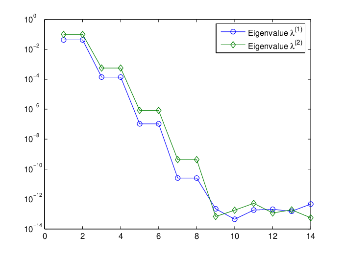
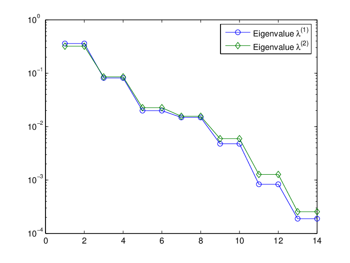
The numerical results for $\Omega_{1}$ are given in table 1. The graphs in Figures 9–11, seem to indicate exponential convergence. For the graphs of $\angle(u_{n}^{(i)},u_{15}^{(i)})$ , see Figure 10. We remark that we use the function $\arccos(x)$ to calculate the angle, and for $n\approx 9$ the numerical calculations give $x=1$ , so the calculated angle becomes $0$ . For the approximation of $R_{n}^{(i)}$ one has to remember that we use a difference method of order $O(h^{2})$ to approximate the Laplace operator, so we can not expect any result better than $10^{-8}$ if we use $h=0.0001$ .

As we expect, the approximations for $\Omega_{2}$ with the transformation $\Phi_{2}$ present a bigger problem for our method. Still from the graphs in Figure 12 and 13 we might infer that the convergence is exponential, but with a smaller exponent than for $\Omega_{1}$ . Because $\Phi_{2}\in C^{4}(B_{3})$ we know that the transformed eigenfunctions on $B_{3}$ are in general only $C^{4}$ , so we can only expect a convergence of $O(n^{-4})$ . The values of $n$ which we use are too small to show what we believe is the true behavior of the $R_{n}^{(i)}$ , although the values for $n=10\ldots 14$ seem to indicate some convergence of the type we would expect.

The poorer convergence for $\Omega_{2}$ as compared to $\Omega_{1}$ illustrates a general problem. When defining a surface $\partial\Omega$ by giving it as the image of a 1-1 mapping from the unit sphere $S^{2}$ into $\mathbb{R}^{3}$ , how does one extend it to a smooth mapping from the unit ball to $\Omega$ ? The mapping in (64) is smooth, but it has large changes in its derivatives, and this affects the rate of convergence of our spectral method. We are working at present on this problem, developing a numerical method to find a well-behaved polynomial mapping $\Phi$ when given only its restriction to $S^{2}$ .

References

[1] M. Abramowitz, I.A. Stegun, Handbook of Mathematical Functions, Dover Publications, Inc., New York, 1965.
[2] K. Atkinson. The numerical solution of the eigenvalue problem for compact integral operators, Trans. Amer. Math. Soc. 129 (1967), 458-465.
[3] K. Atkinson. Convergence rates for approximate eigenvalues of compact integral operators, SIAM J. Num. Anal. 12 (1975), 213-222.
[4] K. Atkinson. The Numerical Solution of Integral Equations of the Second Kind, Cambridge Univ. Press, 1997.
[5] K. Atkinson, D. Chien, and O. Hansen. A Spectral Method for Elliptic Equations: The Dirichlet Problem, Advances in Computational Mathematics, DOI: 10.1007/s10444-009-9125-8, to appear.
[6] K. Atkinson, D. Chien, and O. Hansen. A Spectral Method for Elliptic Equations: The Neumann Problem, submitted for publication. Available from http://arxiv.org/PS_cache/arxiv/pdf/0907/0907.1270v1.pdf.
[7] K. Atkinson and W. Han. Theoretical Numerical Analysis: A Functional Analysis Framework, 2 ${}^{\text{nd}}$ ed., Springer-Verlag, New York, 2005.
[8] K. Atkinson and O. Hansen. Solving the nonlinear Poisson equation on the unit disk, Journal of Integral Equations & Applications, 17 (2005), 223-241.
[9] T. Bagby, L. Bos, and N. Levenberg, Multivariate simultaneous approximation, Constructive Approximation, 18 (2002), pp. 569-577.
[10] J. Boyd. Chebyshev and Fourier Spectral Methods, 2 ${}^{\text{nd}}$ ed., Dover Pub., New York, 2000.
[11] S. Brenner and L. R. Scott. The Mathematical Theory of Finite Element Methods, 2 ${}^{\text{nd}}$ ed., Springer-Verlag, New York, 2002.
[12] C. Canuto, A. Quarteroni, My. Hussaini, and T. Zang, Spectral Methods in Fluid Mechanics, Springer-Verlag, 1988.
[13] C. Canuto, A. Quarteroni, My. Hussaini, and T. Zang, Spectral Methods - Fundamentals in Single Domains, Springer-Verlag, 2006.
[14] F. Chatelin. Spectral Approximation of Linear Operators, Academic Press, 1983.
[15] C. Dunkl and Y. Xu. Orthogonal Polynomials of Several Variables, Cambridge Univ. Press, Cambridge, 2001.
[16] L. Evans. Partial Differential Equations, Amer. Math. Soc., 1998.
[17] W. Gautschi, Orthogonal Polynomials, Oxford University Press, Oxford, 2004.
[18] O. Hansen, K. Atkinson, and D. Chien. On the norm of the hyperinterpolation operator on the unit disk and its use for the solution of the nonlinear Poisson equation, IMA J. Numerical Analysis 29 (2009), 257-283, DOI: 10.1093/imanum/drm052.
[19] E.W. Hobson, The Theory of Spherical and Ellipsoidal Harmonics, Chelsea Publishing Company, New York, 1965.
[20] M. Krasnoselskii. Topological Methods in the Theory of Nonlinear Integral Equations, Pergamon Press, 1964.
[21] O. Ladyzhenskaya and N. Uralt’seva. Linear and Quasilinear Elliptic Equations, Academic Press, 1973.
[22] B. Logan. and L. Shepp. Optimal reconstruction of a function from its projections, Duke Mathematical Journal 42, (1975), 645–659.
[23] T. M. MacRobert, Spherical Harmonics, Dover Publications, Inc., New York, 1948.
[24] S. Mikhlin. Mathematical Physics: An Advanced Course, North-Holland, 1970.
[25] J. Osborn. Spectral approximation for compact operators, Mathematics of Computation 29 (1975), 712-725.
[26] D. Ragozin. Constructive polynomial approximation on spheres and projective spaces, Trans. Amer. Math. Soc. 162 (1971), 157-170.
[27] J. Shen and T. Tang. Spectral and High-Order Methods with Applications, Science Press, Beijing, 2006.
[28] A. Stroud. Approximate Calculation of Multiple Integrals, Prentice-Hall, Inc., Englewood Cliffs, N.J., 1971.
[29] H. Triebel. Higher Analysis, Hüthig Pub. Ltd., 1997.
[30] Yuan Xu. Lecture notes on orthogonal polynomials of several variables, in Advances in the Theory of Special Functions and Orthogonal Polynomials, Nova Science Publishers, 2004, 135-188.
[31] Yuan Xu. Analysis on the unit ball and on the simplex, Electronic Trans. on Numer. Anal. 25 (2006), 284-301.
[32] S. Zhang, J. Jin, Computation of Special Functions, John Wiley & Sons, Inc., New York, 1996.

	$\displaystyle\\|v\\|_{H_{0}^{1}\left(\Omega\right)}^{2}$	$\displaystyle=\int_{\Omega}\left[\left\|\nabla v\left(s\right)\right\|^{2}+\left\|v(s)\right\|^{2}\right]ds$
		$\displaystyle=\int_{B_{d}}\left[\left\|\nabla\widetilde{v}\left(x\right)^{\text{T}}J\left(x\right)^{-1}J\left(x\right)^{-\text{T}}\nabla\widetilde{v}\left(x\right)\right\|+\left\|\widetilde{v}(x)\right\|^{2}\right]\left\|\det J(x)\right\|\,dx$
		$\displaystyle\leq\left[\max_{x\in B}\left\|\det J(x)\right\|\right]\max\left\{\max_{x\in B}\\|J\left(x\right)^{-1}\\|^{2},1\right\}\int_{B_{d}}\left[\left\|\nabla\widetilde{v}\left(x\right)\right\|^{2}+\left\|\widetilde{v}(x)\right\|^{2}\right]\,dx$