跳到论文正文
W Papers独立论文阅读器 arXiv:0909.3121 论文正文 计算阅读时间 · 0%
引用这篇论文根据当前论文元数据生成,正式投稿前建议核对。


License: arXiv.org perpetual non-exclusive license
arXiv:0909.3121v1 [hep-ph] 16 Sep 2009

Pion photoproduction in a nonrelativistic theory

Andreas Fuhrer Address: University of California, San Diego
9500 Gilman Drive, La Jolla, CA 92093–0319
Abstract

The pion and nucleon mass differences generate a very pronounced cusp in the photoproduction reaction of a single pion on the nucleon. A nonrelativistic effective field theory to describe this reaction is constructed. The approach is rigorous in the sense that it is an effective field theory with a consistent power counting scheme. Expressions for the SS- and PP-wave multipole amplitudes for all four reaction channels at two loops are given.

Keywords: 
Chiral symmetries , Meson production , Pion-baryon interactions
PACS
11.30.Rd, 13.60.Le, 13.75.Gx

1. Isospin breaking effects have recently received a considerable amount of attention. This was triggered by the observation of a cusp-like structure in the decay rate of K→3​πK\to 3\pi decays [1], which originates from isospin breaking. Since the strength of this cusp is intimately related to the π​π\pi\pi scattering lengths, another possibility to measure the π​π\pi\pi-scattering lengths – beside Ke​4K_{e4} decays [2, 3] and the lifetime of the pionium atom [4] – was established. It is amusing to note that the same effect that is responsible for the cusp in K→3​πK\to 3\pi decays also leads to a correction to the π​π\pi\pi-scattering phase shifts from Ke​4K_{e4} decays [5].
The photoproduction reaction of neutral pions on the proton is a reaction where isospin breaking corrections have not yet been calculated in a fully systematic approach. On the other hand, it has been known for a long time that this reaction shows a very strong effect due to isospin breaking: the electric multipole E0+E_{0+} exhibits an exceptionally strong cusp at the π+​n\pi^{+}n threshold (see for instance Ref. [6]). In much the same way as in K→3​πK\to 3\pi decays, a nonrelativistic theory – adapted in this letter to the photoproduction reaction of pions on nucleons – provides a rigorous framework which yields quantum field theoretical matrix elements with the effective range parameters of pion-nucleon scattering and the threshold parameters of the photoproduction reaction as free parameters. Furthermore, the framework allows one to include radiative corrections in a standard manner at a later stage.

The cusp in neutral pion photoproduction has been studied before. Ref. [7] introduces a two-parameter model, which captures the most important leading effect of the cusp. In Ref. [8], a coupled channel SS-matrix approach is used to investigate the cusp structure.

In a first step, the nonrelativistic Lagrangian is written down and the power counting is discussed. Then, the coupling constants are matched to the pertinent threshold parameters. The calculation of the multipole amplitudes up to two-loop order is then straightforward. The representation of the amplitudes correctly reproduces the analytical structure in the low energy region. As an application, the relation of the phase of the electric multipole E0+E_{0+} to the phase of the SS-wave of π0​p→π0​p\pi^{0}p\to\pi^{0}p scattering is discussed.

2. Some basic relations and definitions used in the analysis of pion photoproduction are collected. We calculate the matrix element for the process N⁡(p1)+γ⁡(k)→N⁡(p2)+π0,±​(q)N(p_{1})+\gamma(k)\to N(p_{2})+\pi^{0,\pm}(q) for all four channels at leading order in the electromagnetic coupling ee,

⟨p2,qout|p1,kin⟩\displaystyle\langle p_{2},q\,\,\mathrm{out}|p_{1},k\,\,\mathrm{in}\rangle =−i​(2​π)4​δ(4)​(Pf−Pi)​u¯​(p2,t′)​ϵμ​Jμ​u​(p1,t),\displaystyle=-i(2\pi)^{4}\delta^{(4)}(P_{f}-P_{i})\,\bar{u}(p_{2},t^{\prime})\epsilon_{\mu}J^{\mu}u(p_{1},t)\,, (1)

where NN denotes either a proton or a neutron, PiP_{i} and PfP_{f} denote the total four momentum in the initial and in the final state, respectively and ϵμ\epsilon^{\mu} stands for the polarization vector of the photon. In the following, the four reaction channels will be abbreviated as

γ​p→p​π0\displaystyle\gamma p\to p\pi^{0} :(p​0),\displaystyle:(p0)\,, γ​p→n​π+\displaystyle\gamma p\to n\pi^{+} :(n+),\displaystyle:(n+)\,, γ​n→n​π0\displaystyle\gamma n\to n\pi^{0} :(n​0),\displaystyle:(n0)\,, γ​n→p​π−\displaystyle\gamma n\to p\pi^{-} :(p−).\displaystyle:(p-)\,.

To analyze the photoproduction reaction of pions, electric and magnetic multipoles are usually introduced. To this end, the amplitude is written in terms of two component spinors ξt\xi_{t} and Pauli matrices τk\tau^{k} [9],

ℳ\displaystyle\mathcal{M} =8​π​s​ξt′†​ℱ​ξt,\displaystyle=8\pi\sqrt{s}\,\xi^{\dagger}_{t^{\prime}}\,\mathcal{F}\,\xi_{t}\,,
ℱ\displaystyle\mathcal{F} =i​𝝉⋅ϵ​ℱ1+𝝉⋅𝐪^​𝝉⋅(𝐤^×ϵ)​ℱ2+i​𝝉⋅𝐤^​𝐪^⋅ϵ​ℱ3+i​𝝉⋅𝐪^​𝐪^⋅ϵ​ℱ4.\displaystyle=i\boldsymbol{\tau}\cdot\boldsymbol{\epsilon}\,\mathcal{F}_{1}+\boldsymbol{\tau}\cdot\hat{{\bf q}}\,\boldsymbol{\tau}\cdot(\hat{{\bf k}}\times\boldsymbol{\epsilon})\,\mathcal{F}_{2}+i\boldsymbol{\tau}\cdot\hat{{\bf k}}\,\hat{{\bf q}}\cdot\boldsymbol{\epsilon}\,\mathcal{F}_{3}+i\boldsymbol{\tau}\cdot\hat{{\bf q}}\,\hat{{\bf q}}\cdot\boldsymbol{\epsilon}\,\mathcal{F}_{4}\,. (2)

The hat denotes unit vectors. The ℱi\mathcal{F}_{i} are decomposed into electric and magnetic multipoles with the help of derivatives of the Legendre polynomials Pl​(z)P_{l}(z) [9],

ℱ1\displaystyle\mathcal{F}_{1} =∑l=0[l​Ml++El+]​Pl+1′​(z)+[(l+1)​Ml−+El−]​Pl−1′​(z),\displaystyle=\sum_{l=0}\,[lM_{l+}+E_{l+}]P_{l+1}^{\prime}(z)+[(l+1)M_{l-}+E_{l-}]P_{l-1}^{\prime}(z)\,,
ℱ2\displaystyle\mathcal{F}_{2} =∑l=1[(l+1)​Ml++l​Ml−]​Pl′​(z),\displaystyle=\sum_{l=1}\,[(l+1)M_{l+}+lM_{l-}]P_{l}^{\prime}(z)\,,
ℱ3\displaystyle\mathcal{F}_{3} =∑l=1[El+−Ml+]​Pl+1′′​(z)+[El−+Ml−]​Pl−1′′​(z),\displaystyle=\sum_{l=1}\,[E_{l+}-M_{l+}]P_{l+1}^{\prime\prime}(z)+[E_{l-}+M_{l-}]P_{l-1}^{\prime\prime}(z)\,,
ℱ4\displaystyle\mathcal{F}_{4} =∑l=1[Ml+−El+−Ml−−El−]​Pl′′​(z).\displaystyle=\sum_{l=1}\,[M_{l+}-E_{l+}-M_{l-}-E_{l-}]P_{l}^{\prime\prime}(z)\,. (3)

The discussion is restrained to the center of mass frame in the rest of the article.

3. To describe the behavior of the multipoles close to threshold – where the energy of the produced pion and of the nucleon are small – a nonrelativistic calculation is justified. Furthermore, it offers the advantage that all the masses can be set to their physical value. Therefore, all the poles and branch points appear at the correct place in the Mandelstam plane. Moreover, the interaction of the nucleon and the pion is described by effective range parameters, which allows one to directly access the pion-nucleon scattering lengths.

The covariant formulation of nonrelativistic field theories introduced inRefs. [10, 11, 12] is used here since it incorporates the correct relativistic dispersion law for the particles. The nonrelativistic proton, neutron and pion fields are denoted by ψ\psi, χ\chi and πk\pi_{k}, respectively. The kinetic part of the Lagrangian after minimal substitution takes the form (see Ref. [13])

ℒk​i​n\displaystyle\mathcal{L}_{kin} =∑±(i​π±†​Dt​𝒲±​π±−i​(Dt​𝒲±​π±)†​π±−2​π±†​𝒲±2​π±)\displaystyle=\sum_{\pm}\Bigl(i\pi_{\pm}^{\dagger}D_{t}{\cal W}_{\pm}\pi_{\pm}-i(D_{t}{\cal W}_{\pm}\pi_{\pm})^{\dagger}\pi_{\pm}-2\pi_{\pm}^{\dagger}{\cal W}_{\pm}^{2}\pi_{\pm}\Bigr)
+i​ψ†​Dt​𝒲p​ψ−i​(Dt​𝒲p​ψ)†​ψ−2​ψ†​𝒲p2​ψ\displaystyle+i\psi^{\dagger}D_{t}{\cal W}_{p}\psi-i(D_{t}{\cal W}_{p}\psi)^{\dagger}\psi-2\psi^{\dagger}{\cal W}_{p}^{2}\psi
+2χ†Wn(i∂t−Wn)χ+2π0†W0(i∂t−W0)π0,\displaystyle+2\chi^{\dagger}W_{n}(i\partial_{t}-W_{n})\chi+2\pi_{0}^{\dagger}W_{0}(i\partial_{t}-W_{0})\pi_{0}\,, (4)

with

W0\displaystyle W_{0} =Mπ02−△,\displaystyle=\sqrt{M_{\pi^{0}}^{2}-\triangle}\,, Wn\displaystyle W_{n} =mn2−△,\displaystyle=\sqrt{m_{n}^{2}-\triangle}\,, Dt​π±\displaystyle D_{t}\pi_{\pm} =(∂t∓ieA0)π±,\displaystyle=(\partial_{t}\mp ieA_{0})\pi_{\pm}\,,
Dt​ψ\displaystyle D_{t}\psi =(∂t−ieA0)ψ,\displaystyle=(\partial_{t}-ieA_{0})\psi\,, 𝒲±\displaystyle{\cal W}_{\pm} =Mπ2−𝐃2,\displaystyle=\sqrt{M_{\pi}^{2}-{\bf D}^{2}}\,, 𝒲p\displaystyle{\cal W}_{p} =mp2−𝐃2,\displaystyle=\sqrt{m_{p}^{2}-{\bf D}^{2}}\,,
𝐃​π±\displaystyle{\bf D}\pi_{\pm} =(∇±i​e​𝐀)​π±,\displaystyle=(\nabla\pm ie{\bf A})\pi_{\pm}\,, 𝐃​ψ\displaystyle{\bf D}\psi =(∇+i​e​𝐀)​ψ.\displaystyle=(\nabla+ie{\bf A})\psi\,. (5)

Note that since the photon is treated as an external field, its kinetic term is absent.

4. Consider the reaction11 1 The arguments remain of course the same for the other three channel. p⁡(p1)+γ⁡(k)→p⁡(p2)+π0​(q)p(p_{1})+\gamma(k)\to p(p_{2})+\pi^{0}(q). Close to threshold, the momenta of the incoming proton and photon are of the order of the pion mass whereas the outgoing particles have very small momenta. Therefore, we count momenta of the outgoing pion and the outgoing proton as a small quantity of O⁡(ϵ)O(\epsilon) and the momenta of the incoming proton and of the photon as O⁡(1)O(1). All the masses are counted as O⁡(1)O(1). The mass differences of the charged and neutral pion, Δπ≡Mπ2−Mπ02\Delta_{\pi}\equiv M_{\pi}^{2}-M_{\pi^{0}}^{2} and of the proton and the neutron, ΔN≡mn2−mp2\Delta_{N}\equiv m_{n}^{2}-m_{p}^{2} are counted as O⁡(ϵ2)O(\epsilon^{2}). We refrain from counting the pion mass as a small quantity with respect to the nucleon mass, since considering a particle as light and nonetheless describing it nonrelativistically seems inconsistent (see also Ref. [14]).
At first sight, this counting scheme seems to lead to infinitely many terms already in the leading order p+γ→p+π0p+\gamma\to p+\pi^{0} Lagrangian ℒγ\mathcal{L}_{\gamma} because derivatives on the incoming fields are not suppressed in ϵ\epsilon. However, since the the modulus of the momentum of the incoming particles, |𝐤||{\bf k}|, can be expanded in the small momentum |𝐪||{\bf q}|,

|𝐤|\displaystyle|{\bf k}| =∑nkn​𝐪2​n,\displaystyle=\sum_{n}k_{n}{\bf q}^{2n}\,, k0\displaystyle k_{0} =Mπ02​2+y1+y,\displaystyle=\frac{M_{\pi^{0}}}{2}\,\frac{2+y}{1+y}\,, k1\displaystyle k_{1} =y2+2​y+24​Mπ0​(1+y),\displaystyle=\frac{y^{2}+2y+2}{4M_{\pi^{0}}(1+y)}\,, y\displaystyle y =Mπ0mp,\displaystyle=\frac{M_{\pi^{0}}}{m_{p}}\,, (6)

one obtains a valid power counting scheme: Consider the Feynman rule in momentum space of an operator of order O⁡(ϵ0)O(\epsilon^{0}) with a given arbitrary number of derivatives. This expression can be expanded in a sum of one term of order O⁡(ϵ0)O(\epsilon^{0}) without any momenta of the incoming particles present and subsequent higher order terms. Doing this for every operator of O⁡(ϵ0)O(\epsilon^{0}), all the resulting leading order terms without any momentum dependence can be described by one operator of order O⁡(ϵ0)O(\epsilon^{0}) in the interaction Lagrangian. The same procedure leads to finite numbers of operators at any given higher order in ϵ\epsilon. The derivatives on the incoming fields are only needed to generate unit vectors in the direction of the incoming photon. This shows that the nonrelativistic theory is not capable of predicting the dependence on |𝐤||{\bf k}| even at threshold.
An additional generic parameter aa is introduced to count the pion-nucleon scattering vertices. Every pion-nucleon interaction vertex counts as a quantity of order O⁡(a)O(a) since the coupling constants are proportional to the pion-nucleon scattering threshold parameters, which are small. The perturbative expansion is therefore a combined expansion in ϵ\epsilon and aa.

5. The Lagrangian needed for the calculation of the amplitudes for pion photoproduction reads ℒ=ℒk​i​n+ℒγ+ℒπ​N\mathcal{L}=\mathcal{L}_{kin}+\mathcal{L}_{\gamma}+\mathcal{L}_{\pi N}, where ℒk​i​n\mathcal{L}_{kin} denotes the kinetic part, ℒγ\mathcal{L}_{\gamma} incorporates the interaction with the photon field and and ℒπ​N\mathcal{L}_{\pi N} describes the pion-nucleon sector.

In the pion nucleon sector, the leading terms of the Lagrangian have been given before in Ref. [15]. First, some notation is introduced in order to write the Lagrangian in a compact form. For every channel nn, we collect the charges of the outgoing and the incoming pions in the variables vv and ww, (n,v,w)(n;v,w): (0;0,0),(1;0,+),(2;+,+),(3;0,0),(4;−,0),(5;−,−)(0;0,0),(1;0,+),\,(2;+,+),\,(3;0,0),\,(4;-,0),\,(5;-,-), thereby assigning unique values to the variables vv and ww once nn is given. The Lagrangian reads

ℒπ​N\displaystyle\mathcal{L}_{\pi N} =(ψ†​χ†)​(T{0,5}T{1,4}T{1,4}†T{2,3})​(ψχ),\displaystyle=\left(\psi^{\dagger}\,\,\chi^{\dagger}\right)\left(\begin{array}[]{cc}T_{\{0,5\}}&T_{\{1,4\}}\\ T_{\{1,4\}}^{\dagger}&T_{\{2,3\}}\end{array}\right)\left(\begin{array}[]{c}\psi\\ \chi\end{array}\right)\,,
T𝒞\displaystyle T_{\mathcal{C}} =∑n∈𝒞[Cn​πv†​πw+Dn(1)​∇kπv†​∇kπw+Dn(2)​πv†​△↔​πw+i​Dn(3)​τk​ϵi​j​k​∇iπv†​∇jπw]\displaystyle=\sum_{n\in\,\mathcal{C}}\left[C_{n}\pi_{v}^{\dagger}\pi_{w}+D_{n}^{(1)}\nabla^{k}\pi^{\dagger}_{v}\nabla^{k}\pi_{w}+D_{n}^{(2)}\pi^{\dagger}_{v}\overleftrightarrow{\triangle}\pi_{w}+iD_{n}^{(3)}\tau^{k}\epsilon^{ijk}\nabla^{i}\pi^{\dagger}_{v}\nabla^{j}\pi_{w}\right]

with the abbreviation f​△↔​g≡f​△​g+(△​f)​gf\overleftrightarrow{\triangle}g\equiv f\triangle g+(\triangle f)g.
For ℒγ\mathcal{L}_{\gamma}, the photon is treated as an external vector field 𝐀{\bf A} which is odd under parity and time-reversal transformations. Gauge invariance requires that it can only appear in covariant derivatives and through the Maxwell equations in the electric and magnetic field 𝐄=−∇A0−𝐀˙{\bf E}=-\boldsymbol{\nabla}A^{0}-\dot{{\bf A}} and 𝐁=∇×𝐀{\bf B}=\boldsymbol{\nabla}\times{\bf A}. The interaction Lagrangian can be read off from the nonrelativistically reduced and multipole expanded matrix element, Eq. (2) and the known threshold behavior of the multipoles, El±,Ml±∼|𝐪|lE_{l\pm},M_{l\pm}\sim|{\bf q}|^{l}. As already mentioned, the effective theory fails to predict the dependence on |𝐤||{\bf k}| even at threshold. Factors of |𝐤||{\bf k}| can always be obtained by a redefinition of the coupling constants of the Lagrangian. Of course, all the terms have to be invariant under space rotations, parity and time reversal transformations. This leads to the following expression for the Lagrangian ℒγ\mathcal{L}_{\gamma}. The upper index on the coupling constants counts the number of derivatives on the external vector field and is introduced for later convenience.

ℒγ(0)\displaystyle\mathcal{L}^{(0)}_{\gamma} =−i​G0(1)​ψ†​τk​ψ​Ek​π0†\displaystyle=-iG_{0}^{(1)}\psi^{\dagger}\tau^{k}\psi\,E^{k}\,\pi_{0}^{\dagger}
ℒγ(1)\displaystyle\mathcal{L}^{(1)}_{\gamma} =−i​G1(2)​ψ†​τk​ψ​∇jEk​∇jπ0†+i​G2(1)​ψ†​τm​τl​ψ​Bl​∇mπ0†\displaystyle=-iG_{1}^{(2)}\,\psi^{\dagger}\tau^{k}\psi\,\nabla^{j}E^{k}\,\nabla^{j}\pi_{0}^{\dagger}+iG_{2}^{(1)}\,\psi^{\dagger}\tau^{m}\tau^{l}\psi\,B^{l}\,\nabla^{m}\pi_{0}^{\dagger}
−i​G3(2)​ψ†​τj​ψ​∇jEk​∇kπ0†\displaystyle-iG_{3}^{(2)}\,\psi^{\dagger}\tau^{j}\psi\,\nabla^{j}E^{k}\,\nabla^{k}\pi_{0}^{\dagger}
ℒγ(2)\displaystyle\mathcal{L}^{(2)}_{\gamma} =−i​G4(3)​ψ†​τk​ψ​∇j​lEk​∇j​lπ0†−i​G5(1)​ψ†​τk​ψ​Ek​△​π0†\displaystyle=-iG_{4}^{(3)}\psi^{\dagger}\tau^{k}\psi\nabla^{jl}E^{k}\nabla^{jl}\pi_{0}^{\dagger}-iG_{5}^{(1)}\psi^{\dagger}\tau^{k}\psi E^{k}\triangle\pi_{0}^{\dagger}
+i​G6(2)​ψ†​τm​τl​ψ​∇nBl​∇m​nπ0†−i​G7(3)​ψ†​τj​ψ​∇j​lEk​∇k​lπ0†\displaystyle+iG_{6}^{(2)}\psi^{\dagger}\tau^{m}\tau^{l}\psi\nabla^{n}B^{l}\nabla^{mn}\pi_{0}^{\dagger}-iG_{7}^{(3)}\psi^{\dagger}\tau^{j}\psi\nabla^{jl}E^{k}\nabla^{kl}\pi_{0}^{\dagger}
−i​G8(1)​ψ†​τj​ψ​Ek​∇j​kπ0†\displaystyle-iG_{8}^{(1)}\psi^{\dagger}\tau^{j}\psi E^{k}\nabla^{jk}\pi_{0}^{\dagger}
ℒγ(3)\displaystyle\mathcal{L}^{(3)}_{\gamma} =−i​G9(2)​ψ†​τk​ψ​∇jEk​△​∇jπ0†−i​G10(4)​ψ†​τk​ψ​∇l​m​nEk​∇l​m​nπ0†\displaystyle=-iG_{9}^{(2)}\psi^{\dagger}\tau^{k}\psi\nabla^{j}E^{k}\triangle\nabla^{j}\pi_{0}^{\dagger}-iG_{10}^{(4)}\psi^{\dagger}\tau^{k}\psi\nabla^{lmn}E^{k}\nabla^{lmn}\pi_{0}^{\dagger}
+i​G11(1)​ψ†​τm​τl​ψ​Bl​△​∇mπ0†+i​G12(3)​ψ†​τm​τl​ψ​∇i​nBl​∇m​i​nπ0†\displaystyle+iG_{11}^{(1)}\psi^{\dagger}\tau^{m}\tau^{l}\psi B^{l}\triangle\nabla^{m}\pi_{0}^{\dagger}+iG_{12}^{(3)}\psi^{\dagger}\tau^{m}\tau^{l}\psi\nabla^{in}B^{l}\nabla^{min}\pi_{0}^{\dagger}
−i​G13(2)​ψ†​τj​ψ​∇jEk​△​∇kπ0†−i​G14(4)​ψ†​τj​ψ​∇j​l​mEk​∇k​l​mπ0†\displaystyle-iG_{13}^{(2)}\psi^{\dagger}\tau^{j}\psi\nabla^{j}E^{k}\triangle\nabla^{k}\pi_{0}^{\dagger}-iG_{14}^{(4)}\psi^{\dagger}\tau^{j}\psi\nabla^{jlm}E^{k}\nabla^{klm}\pi_{0}^{\dagger}
−i​G15(2)​ψ†​τj​ψ​∇lEk​∇j​k​lπ0†\displaystyle-iG_{15}^{(2)}\psi^{\dagger}\tau^{j}\psi\nabla^{l}E^{k}\nabla^{jkl}\pi_{0}^{\dagger} (11)

Here, the notation ∇i1​i2​…​ik≡∇i1∇i2⋯∇ik\nabla^{i_{1}i_{2}\ldots i_{k}}\equiv\nabla^{i_{1}}\nabla^{i_{2}}\cdots\nabla^{i_{k}} is used. Since the structure of the Lagrangian for the remaining channels stays the same, one only has to replace the coupling constants and the field operators,

(n+)\displaystyle(n+) :{ψ†,π0†,Gi(n)}→{χ†,π+†,Hi(n)},\displaystyle:\{\psi^{\dagger},\pi_{0}^{\dagger},G_{i}^{(n)}\}\to\{\chi^{\dagger},\pi_{+}^{\dagger},H_{i}^{(n)}\}\,, (n​0)\displaystyle(n0) :{ψ,ψ†,Gi(n)}→{χ,χ†,Li(n)},\displaystyle:\{\psi,\psi^{\dagger},G_{i}^{(n)}\}\to\{\chi,\chi^{\dagger},L_{i}^{(n)}\}\,,
(p−)\displaystyle(p-) :{ψ,π0†,Gi(n)}→{χ,π−†,Ki(n)}.\displaystyle:\{\psi,\pi_{0}^{\dagger},G_{i}^{(n)}\}\to\{\chi,\pi_{-}^{\dagger},K_{i}^{(n)}\}\,. (12)

The full interaction Lagrangian ℒγ\mathcal{L}_{\gamma} is then given by adding the ℒγ(i)\mathcal{L}^{(i)}_{\gamma} of all four channels.

Here, a remark about the structure of the interaction terms seems in order. Since the interaction Lagrangian contains by construction no π​N​N\pi NN couplings, there is no nucleon pole diagram.

Refer to caption
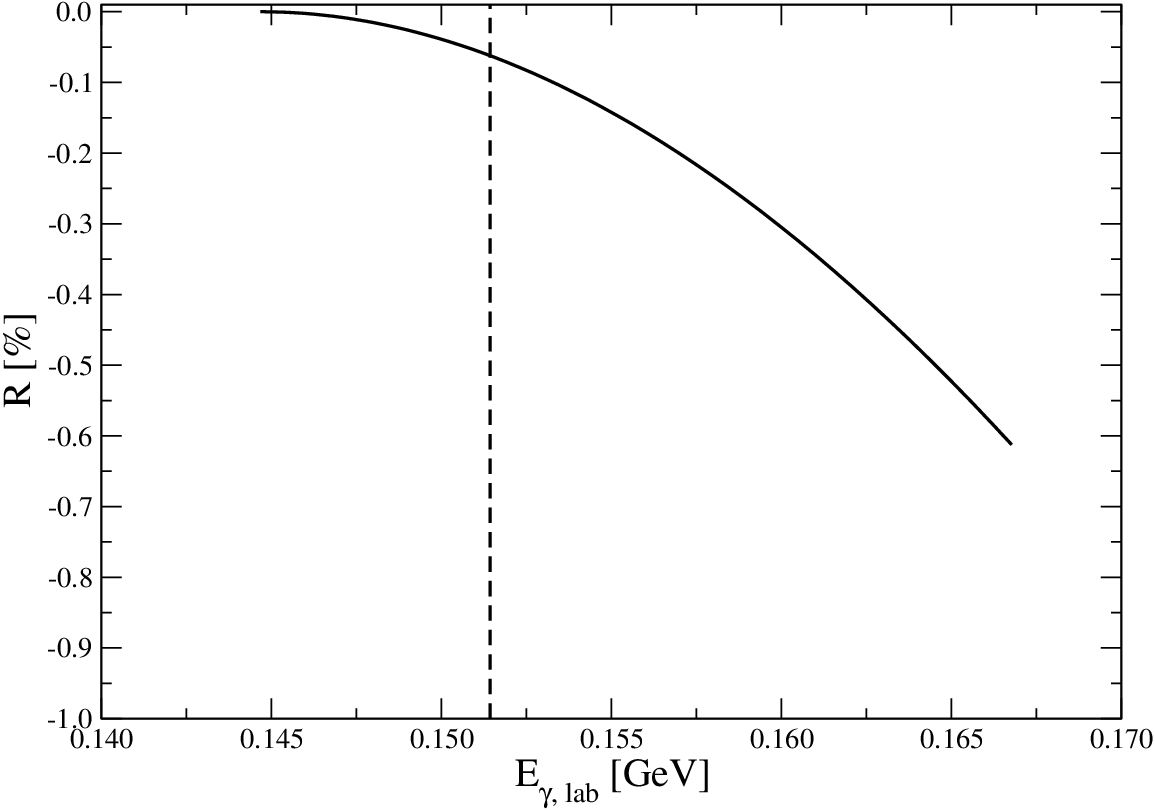
Figure 1: The ratio RR plotted as a function of the photon energy in the lab frame. The dashed line shows the n​π+n\pi^{+} threshold.

Therefore one might be worried that an expansion in powers of the momentum 𝐪{\bf q} does not converge sufficiently fast even in a vicinity of the threshold. However, we check explicitly that the nucleon pole in the ss channel can be approximated by a polynomial in 𝐪{\bf q}. The tree level expressions of E0+E_{0+} in the channel (p​0)(p0) (taken from Ref. [7]) expanded up to and including terms of order 𝐪2{\bf q}^{2} yields a good approximation of the full tree level result. In Fig. 1, the ratio R=(E0+exp.−E0+)/E0+R=(E_{0+}^{\mathrm{exp.}}-E_{0+})/E_{0+} is plotted as a function of the photon energy in the rest frame of the proton. In view of this result, we also conclude that there is no reason to be concerned about singularities from resonances like the ρ\rho in the tt channel or the Δ⁡(1232)\Delta(1232) in the ss channel, which are almost as close to threshold.

6. In the pion-nucleon sector, the coupling constants of the nonrelativistic Lagrangian, CiC_{i} and Di(k)D^{(k)}_{i} can be expressed in terms of pion-nucleon scattering lengths of the SS-wave and PP-wave, a0+a_{0+} and a1±a_{1\pm} and effective range parameters b0+b_{0+}, respectively. Adopting the notation of Ref. [16], in the isospin limit, the isospin decomposition of the π​N\pi N scattering amplitudes reads

Tp​π0→p​π0\displaystyle T_{p\pi^{0}\to p\pi^{0}} =Tn​π0→n​π0=T+,\displaystyle=T_{n\pi^{0}\to n\pi^{0}}=T^{+}\,, Tp​π0→n​π+\displaystyle T_{p\pi^{0}\to n\pi^{+}} =Tn​π0→p​π−=−2​T−,\displaystyle=T_{n\pi^{0}\to p\pi^{-}}=-\sqrt{2}\,T^{-}\,,
Tn​π+→n​π+\displaystyle T_{n\pi^{+}\to n\pi^{+}} =Tp​π−→p​π−=T++T−.\displaystyle=T_{p\pi^{-}\to p\pi^{-}}=T^{+}+T^{-}\,. (13)

Defining 𝒩=4​π​(mp+Mπ)\mathcal{N}=4\pi(m_{p}+M_{\pi}), one finds

C0\displaystyle C_{0} =2​𝒩​a0++,\displaystyle=2\,\mathcal{N}a_{0+}^{+}\,, C1\displaystyle C_{1} =2​2​𝒩​a0+−,\displaystyle=2\sqrt{2}\,\mathcal{N}a_{0+}^{-}\,, C2\displaystyle C_{2} =2​𝒩​(a0+++a0+−),\displaystyle=2\,\mathcal{N}(a_{0+}^{+}+a_{0+}^{-})\,,
C3\displaystyle C_{3} =C0,\displaystyle=C_{0}\,, C4\displaystyle C_{4} =C1,\displaystyle=C_{1}\,, C5\displaystyle C_{5} =C2.\displaystyle=C_{2}\,. (14)

The matching conditions for the Di(k)D_{i}^{(k)} are given in a generic form only. The isospin index of the threshold parameters can be inferred from Eq. (13)22 2 Note that we use the Condon-Shortley phase convention..

Di(1)\displaystyle D^{(1)}_{i} =2​𝒩​(2​a1++a1−),\displaystyle=2\mathcal{N}(2a_{1+}+a_{1-})\,, Di(2)\displaystyle D^{(2)}_{i} =−𝒩⁡(a0+2​mp​Mπ+b0+),\displaystyle=-\mathcal{N}\left(\frac{a_{0+}}{2m_{p}M_{\pi}}+b_{0+}\right)\,,
Di(3)\displaystyle D^{(3)}_{i} =2​𝒩​(a1−−a1+).\displaystyle=2\mathcal{N}\ (a_{1-}-a_{1+})\,. (15)

Here, higher order terms in the threshold parameters have been dropped. The corrections to these relations which appear due to isospin breaking have to be calculated within the underlying relativistic theory. For the CiC_{i}, they can be found in Refs. [17, 18, 19]. Note that the second line in Eq. (14) is only true in the isospin limit.

The constants Gi(n)G^{(n)}_{i}, Hi(n)H^{(n)}_{i}, Ki(n)K^{(n)}_{i} and Li(n)L^{(n)}_{i} on the other hand are related to the threshold parameters of the electric and magnetic multipoles of the pertinent channel. In the isospin limit, the expansion of the real part of the multipole Xl±X_{l\pm} close to threshold is written in the form

Re​Xl±​(s)\displaystyle\mathrm{Re}X_{l\pm}(s) =∑k=0∞X¯l±,2​k​|𝐪|l+2​k,\displaystyle=\sum_{k=0}^{\infty}\bar{X}_{l\pm,2k}|{\bf q}|^{l+2k}\,, (16)

which defines the threshold parameters X¯l±,2​k\bar{X}_{l\pm,2k}. In the following, the relations of the coupling constants Gi(n)G^{(n)}_{i} to these threshold parameters is given at leading order in the pion nucleon threshold parameters. Since the nonrelativistic theory is not suited for the study of the dependence of the multipoles on |𝐤||{\bf k}|, in this analysis, all vectors 𝐤{\bf k} are turned into unit vectors by the pertinent redefinition of the coupling constants,

Gi(n)=𝒩0​k0−n​Gi,𝒩0=4​π​(mp+Mπ0).G_{i}^{(n)}=\mathcal{N}_{0}k_{0}^{-n}G_{i}\,,\qquad\mathcal{N}_{0}=4\pi(m_{p}+M_{\pi^{0}})\,. (17)

Note that the higher order corrections due to Eq. (6) are taken care of in the matching relations. Again, these relations pick up isospin breaking corrections which have to be evaluated in the underlying relativistic theory.

Only the matching equations for the couplings of the Lagrangians ℒγ(0)\mathcal{L}_{\gamma}^{(0)} and ℒγ(1)\mathcal{L}_{\gamma}^{(1)} are indicated in the main text, the remaining relations are relegated to appendix A. To ease notation, X¯i±≡X¯i±,0\bar{X}_{i\pm}\equiv\bar{X}_{i\pm,0} is used.

G0\displaystyle G_{0} =2​E¯0+,\displaystyle=2\bar{E}_{0+}\,, G1\displaystyle G_{1} =6​(E¯+1+M¯+1),\displaystyle=6(\bar{E}_{+1}+\bar{M}_{+1})\,,
G2\displaystyle G_{2} =−2​(M¯−1+2​M¯+1),\displaystyle=-2(\bar{M}_{-1}+2\bar{M}_{+1})\,, G3\displaystyle G_{3} =6​(E¯1+−M¯1+).\displaystyle=6(\bar{E}_{1+}-\bar{M}_{1+})\,. (18)

For the coupling constants HiH_{i}, KiK_{i} and LiL_{i}, the algebraic form of the relations is identical. However, the multipoles of the pertinent channels appear and the masses in Eq. (17) have to be adjusted.

Upon the inclusion of dynamical photons, the nonrelativistic coupling constants pick up an imaginary part due to γ​N\gamma N intermediate states (see Ref. [14] for a discussion of this issue). For the coupling constants CiC_{i}, the imaginary part can be obtained from Ref. [19]. The imaginary part of the coupling constants G0G_{0} and H0H_{0} in the photoproduction Lagrangian ℒγ\mathcal{L}_{\gamma} follows from the imaginary parts of E0+E_{0+} at threshold. A calculation at leading order in chiral perturbation theory [20] yields

Im​E0+\displaystyle\mathrm{Im}E_{0+} =e3​g​y​(y+2)64​π2​F​(1+y)112​[1−(y+1)3​ln⁡(1+y)]\displaystyle=\frac{e^{3}g\,y(y+2)}{64\pi^{2}F(1+y)^{\frac{11}{2}}}\bigg[1-(y+1)^{3}\ln(1+y)\bigg] (19)

for the channel (p​0)(p0) and

Im​E0+\displaystyle\mathrm{Im}E_{0+} =e3​g​(y+2)2​ 32​π2​F​(1+y)112​[112​(2​y+5)​(y2+2)−(y+1)3​ln⁡(1+y)]\displaystyle=\frac{e^{3}g(y+2)}{\sqrt{2}\,32\pi^{2}F(1+y)^{\frac{11}{2}}}\bigg[\frac{1}{12}(2y+5)(y^{2}+2)-(y+1)^{3}\ln(1+y)\bigg] (20)

for the channel (n+)(n+). Here, FF and gg denote the pion decay constant and the axial coupling, both in the chiral limit. A comparison with the real part at threshold – which is estimated taking the experimental results from Refs. [21, 22] – shows that the imaginary part is indeed of the generic order of electromagnetic corrections,

Im​G0Re​G0\displaystyle\frac{\mathrm{Im}\,G_{0}}{\mathrm{Re}\,G_{0}} ≃O⁡(10−2),\displaystyle\simeq O(10^{-2})\,, Im​H0Re​H0\displaystyle\frac{\mathrm{Im}\,H_{0}}{\mathrm{Re}\,H_{0}} ≃O⁡(10−3).\displaystyle\simeq O(10^{-3})\,. (21)

In the following, we assume that the coupling constants are real.

7. In the following, we provide the expressions for the electric and magnetic multipoles El+E_{l+} for l=0,1l=0,1 and Ml±M_{l\pm} for l=1l=1 for the channel (p​0)(p0). The result is written in the form

Xl,±​(s)\displaystyle X_{l,\pm}(s) =Xl±tree​(s)+Xl±1​L​o​o​p​(s)+Xl±2​L​o​o​p​(s)+⋯\displaystyle=X_{l\pm}^{\mathrm{tree}}(s)+X_{l\pm}^{\mathrm{1Loop}}(s)+X_{l\pm}^{\mathrm{2Loop}}(s)\cdots (22)

where s=(p1+k)2s=(p_{1}+k)^{2} and the ellipsis denote higher order terms in the expansion in ϵ\epsilon and aa. The results for the other channels can be recovered by a simple replacement of the coupling constants which will be given later. Writing

Xl±tree​(s)\displaystyle X^{\mathrm{tree}}_{l\pm}(s) =Xl±t​𝐪l+Xl±,2t​𝐪2+l+⋯.\displaystyle=X^{t}_{l\pm}{\bf q}^{l}+X^{t}_{l\pm,2}{\bf q}^{2+l}+\cdots\,. (23)

one finds

E0+t\displaystyle E^{t}_{0+} =G0,\displaystyle=G_{0}\,, 3​E0+,2t\displaystyle 3E^{t}_{0+,2} =G4−3​G5+G6−G8,\displaystyle=G_{4}-3G_{5}+G_{6}-G_{8}\,,
6​M1+t\displaystyle 6M^{t}_{1+} =G1−G3,\displaystyle=G_{1}-G_{3}\,, M1+,2t\displaystyle M^{t}_{1+,2} =−16​G9+110​G10+115​G12+16​G13−130​G14,\displaystyle=-\tfrac{1}{6}G_{9}+\tfrac{1}{10}G_{10}+\tfrac{1}{15}G_{12}+\tfrac{1}{6}G_{13}-\tfrac{1}{30}G_{14}\,,
3​M1−t\displaystyle 3M^{t}_{1-} =G3−G1−3​G2,\displaystyle=G_{3}-G_{1}-3G_{2}\,, M1−,2t\displaystyle M^{t}_{1-,2} =13​G9−15​G10+G11−13​G12\displaystyle=\tfrac{1}{3}G_{9}-\tfrac{1}{5}G_{10}+G_{11}-\tfrac{1}{3}G_{12}
−13​G13+115​G14,\displaystyle-\tfrac{1}{3}G_{13}+\tfrac{1}{15}G_{14}\,,
6​E1+t\displaystyle 6E^{t}_{1+} =G1+G3,\displaystyle=G_{1}+G_{3}\,, E1+,2t\displaystyle E^{t}_{1+,2} =−16​G9+110​G10+115​G12−16​G13\displaystyle=-\tfrac{1}{6}G_{9}+\tfrac{1}{10}G_{10}+\tfrac{1}{15}G_{12}-\tfrac{1}{6}G_{13}
+130​G14−115​G15.\displaystyle+\tfrac{1}{30}G_{14}-\tfrac{1}{15}G_{15}\,. (24)

One observes that DD-waves appear naturally at order ϵ2\epsilon^{2} in this framework (see also Ref.[23]).

8. All the one-loop contributions are proportional to the basic integral

Ja​b​(P2)\displaystyle J_{ab}(P^{2}) =∫dD​li​(2​π)D​12​ωa​(𝐥)​2​ωb​(𝐏−𝐥)​1(ωa​(𝐥)−l0)​(ωb​(𝐏−𝐥)−P0+l0),\displaystyle=\int\frac{d^{D}l}{i(2\pi)^{D}}\frac{1}{2\omega_{a}({\bf l})2\omega_{b}({\bf P}-{\bf l})}\,\frac{1}{(\omega_{a}({\bf l})-l_{0})(\omega_{b}({\bf P}-{\bf l})-P_{0}+l_{0})}\,,
ω±​(𝐩)\displaystyle\omega_{\pm}({\bf p}) =Mπ2+𝐩2,\displaystyle=\sqrt{M_{\pi}^{2}+{\bf p}^{2}}\,, ωi​(𝐩)\displaystyle\omega_{i}({\bf p}) =mi2+𝐩2,i=n,p\displaystyle=\sqrt{m_{i}^{2}+{\bf p}^{2}}\,,\qquad i=n,p
ω0​(𝐩)\displaystyle\omega_{0}({\bf p}) =Mπ02+𝐩2,\displaystyle=\sqrt{M_{\pi^{0}}^{2}+{\bf p}^{2}}\,, P2\displaystyle P^{2} =P02−𝐏2.\displaystyle=P_{0}^{2}-{\bf P}^{2}\,. (25)

In the limit D→4D\to 4,

Ja​b​(P2)=i16​π​s​(s−(ma+Mπb)2)​(s−(ma−Mπb)2),J_{ab}(P^{2})=\frac{i}{16\pi s}\sqrt{(s-(m_{a}+M_{\pi^{b}})^{2})(s-(m_{a}-M_{\pi^{b}})^{2})}\,, (26)

which is a quantity of order ϵ\epsilon.

Refer to caption Refer to caption
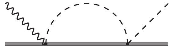
Figure 2: One- and two loop topologies needed to calculate the amplitude. The double line generically denotes a nucleon, the dashed line a pion and the wiggly line indicates the external electromagnetic field.

The one-loop result for channel (c)(c) up to and including order O⁡(a​ϵ4)O(a\epsilon^{4}) reads

(E0+1​L​o​o​p​(s)1|𝐪|​M1+1​L​o​o​p​(s)1|𝐪|​M1−1​L​o​o​p​(s)1|𝐪|​E1+1​L​o​o​p​(s))\displaystyle\left(\begin{array}[]{c}E_{0+}^{\mathrm{1Loop}}(s)\\ \frac{1}{|{\bf q}|}M_{1+}^{\mathrm{1Loop}}(s)\\ \frac{1}{|{\bf q}|}M_{1-}^{\mathrm{1Loop}}(s)\\ \frac{1}{|{\bf q}|}E_{1+}^{\mathrm{1Loop}}(s)\end{array}\right) =(P11(c)P12(c)P21(c)P22(c)P31(c)P32(c)P41(c)P42(c))​(Ja​b​(s)Jc​d​(s)),\displaystyle=\left(\begin{array}[]{cc}P^{(c)}_{11}&P^{(c)}_{12}\\ P_{21}^{(c)}&P^{(c)}_{22}\\ P^{(c)}_{31}&P^{(c)}_{32}\\ P^{(c)}_{41}&P^{(c)}_{42}\end{array}\right)\left(\begin{array}[]{c}J_{ab}(s)\\ J_{cd}(s)\end{array}\right)\,,

where ma,Mπbm_{a},M_{\pi^{b}} denote the masses of the final state of the pertinent channel and mc,Mπdm_{c},M_{\pi^{d}} stands for the masses of the intermediate state that differ from the final state masses. The elements Pi​k(c)P^{(c)}_{ik} are functions of the pion momentum 𝐪{\bf q} and the coupling constants of the Lagrangian. For the channel (p​0)(p0), one finds

P11(p​0)\displaystyle P_{11}^{(p0)} =G0​C0+𝐪2​(C0​E0+,2(p​0),t−2​D0(2)​G0),\displaystyle=G_{0}C_{0}+{\bf q}^{2}\left(C_{0}E^{(p0),t}_{0+,2}-2D_{0}^{(2)}G_{0}\right)\,,
P12(p​0)\displaystyle P_{12}^{(p0)} =C1​H0+h2​(s,mc,Mπd)​(C1​E0+,2(n+),t−D1(2)​H0)−𝐪2​D1(2)​H0,\displaystyle=C_{1}H_{0}+h^{2}(s,m_{c},M_{\pi^{d}})\left(C_{1}E^{(n+),t}_{0+,2}-D_{1}^{(2)}H_{0}\right)-{\bf q}^{2}D_{1}^{(2)}H_{0}\,,
18​P21(p​0)\displaystyle 18P_{21}^{(p0)} =𝐪2​(D0(1)−D0(3))​(G1−G3),\displaystyle={\bf q}^{2}\left(D^{(1)}_{0}-D^{(3)}_{0}\right)(G_{1}-G_{3})\,,
18​P22(p​0)\displaystyle 18P_{22}^{(p0)} =h2​(s,mc,Mπd)​(D1(1)−D1(3))​(H1−H3),\displaystyle=h^{2}(s,m_{c},M_{\pi^{d}})\left(D^{(1)}_{1}-D^{(3)}_{1}\right)(H_{1}-H_{3})\,,
9​P31(p​0)\displaystyle 9P_{31}^{(p0)} =𝐪2​(D0(1)+2​D0(3))​(G3−G1−3​G2),\displaystyle={\bf q}^{2}\left(D^{(1)}_{0}+2D^{(3)}_{0}\right)(G_{3}-G_{1}-3G_{2})\,,
9​P32(p​0)\displaystyle 9P_{32}^{(p0)} =h2​(s,mc,Mπd)​(D1(1)+2​D1(3))​(H3−H1−3​H2),\displaystyle=h^{2}(s,m_{c},M_{\pi^{d}})\left(D^{(1)}_{1}+2D^{(3)}_{1}\right)(H_{3}-H_{1}-3H_{2})\,,
18​P41(p​0)\displaystyle 18P_{41}^{(p0)} =𝐪2​(D0(1)−D0(3))​(G1+G3),\displaystyle={\bf q}^{2}\left(D^{(1)}_{0}-D^{(3)}_{0}\right)(G_{1}+G_{3})\,,
18​P42(p​0)\displaystyle 18P_{42}^{(p0)} =h2​(s,mc,Mπd)​(D1(1)−D1(3))​(H1+H3),\displaystyle=h^{2}(s,m_{c},M_{\pi^{d}})\left(D^{(1)}_{1}-D^{(3)}_{1}\right)(H_{1}+H_{3})\,, (37)

where E0+,2(c),tE^{(c),t}_{0+,2} denotes the pertinent coefficient of the tree level result of channel (c)(c), see Eq. (23), and h2​(s,mc,Mπd)h^{2}(s,m_{c},M_{\pi^{d}}) is given by

h2​(s,mc,Mπd)\displaystyle h^{2}(s,m_{c},M_{\pi^{d}}) =(s−(mc+Mπd)2)​(s−(mc−Mπd)2)4​s,\displaystyle=\frac{\left(s-(m_{c}+M_{\pi^{d}})^{2}\right)\left(s-(m_{c}-M_{\pi^{d}})^{2}\right)}{4s}\,, (38)

which is a quantity of order ϵ2\epsilon^{2}. Eq. (Pion photoproduction in a nonrelativistic theory) and (Pion photoproduction in a nonrelativistic theory) clearly show the advantage of the nonrelativistic description: The strength of the cusp in the channel (p​0)(p0) is parameterized in terms of the coupling constant C1C_{1} and the ratio H0/G0H_{0}/G_{0}.

9. The two-loop corrections all have the topology shown in Fig. 2 and can therefore be cast into the form

E0+2​L​o​o​p​(s)\displaystyle E_{0+}^{\mathrm{2Loop}}(s) =(Ja​b​(s)​Jc​d​(s))​(T11(c)T12(c)T12(c)T22(c))​(Ja​b​(s)Jc​d​(s)),\displaystyle=\big(J_{ab}(s)\,\,\,J_{cd}(s)\big)\left(\begin{array}[]{cc}T^{(c)}_{11}&T^{(c)}_{12}\\ T_{12}^{(c)}&T^{(c)}_{22}\end{array}\right)\left(\begin{array}[]{c}J_{ab}(s)\\ J_{cd}(s)\end{array}\right)\,,

where the Ti​j(c)T^{(c)}_{ij} for the channel (p​0)(p0) read

T11(p​0)\displaystyle T_{11}^{(p0)} =C02​G0+C02​E0+,2(p​0),t​𝐪2−4​C0​G0​D0(2)​𝐪2,\displaystyle=C^{2}_{0}G_{0}+C^{2}_{0}E^{(p0),t}_{0+,2}{\bf q}^{2}-4C_{0}G_{0}D_{0}^{(2)}{\bf q}^{2}\,,
T12(p​0)\displaystyle T_{12}^{(p0)} =12​C12​G0+12​C0​C1​H0+12​C12​E0+,2(p​0),t​𝐪2−C1​H0​D0(2)​𝐪2−C1​G0​D1(2)​𝐪2\displaystyle=\frac{1}{2}C_{1}^{2}\,G_{0}+\frac{1}{2}C_{0}\,C_{1}\,H_{0}+\frac{1}{2}C_{1}^{2}\,E^{(p0),t}_{0+,2}{\bf q}^{2}-C_{1}\,H_{0}\,D_{0}^{(2)}{\bf q}^{2}-C_{1}\,G_{0}\,D_{1}^{(2)}{\bf q}^{2}
−12​C0​H0​D1(2)​𝐪2+12​C0​C1​E0+,2(n+),t​h2​(s,mc,Mπd)\displaystyle-\frac{1}{2}C_{0}\,H_{0}\,D_{1}^{(2)}{\bf q}^{2}+\frac{1}{2}C_{0}\,C_{1}\,E^{(n+),t}_{0+,2}\,h^{2}(s,m_{c},M_{\pi^{d}})
−C1​G0​D1(2)​h2​(s,mc,Mπd)−12​C0​H0​D1(2)​h2​(s,mc,Mπd),\displaystyle-C_{1}\,G_{0}\,D_{1}^{(2)}\,h^{2}(s,m_{c},M_{\pi^{d}})-\frac{1}{2}C_{0}\,H_{0}\,D_{1}^{(2)}\,h^{2}(s,m_{c},M_{\pi^{d}})\,,
T22(p​0)\displaystyle T_{22}^{(p0)} =C1​C2​H0−C2​H0​D1(2)​𝐪2+C1​C2​E0+,2(n+),t​h2​(s,mc,Mπd)\displaystyle=C_{1}C_{2}H_{0}-C_{2}H_{0}D_{1}^{(2)}{\bf q}^{2}+C_{1}C_{2}E^{(n+),t}_{0+,2}h^{2}(s,m_{c},M_{\pi^{d}})
−C2​H0​D1(2)​h2​(s,mc,Mπd)−2​C1​H0​D2(2)​h2​(s,mc,Mπd).\displaystyle-C_{2}H_{0}D_{1}^{(2)}h^{2}(s,m_{c},M_{\pi^{d}})-2C_{1}H_{0}D_{2}^{(2)}h^{2}(s,m_{c},M_{\pi^{d}})\,. (43)

Up to and including order O⁡(a2​ϵ5)O(a^{2}\epsilon^{5}), the two-loop corrections are independent of the scattering angle cos⁡Θ\cos\Theta and only contribute to the amplitude ℱ1\mathcal{F}_{1}. Therefore, at the order considered here, the electric multipole E0+E_{0+} is the only quantity which receives two-loop corrections.

10. The result for the other channels are obtained from the tree level result of channel (p​0)(p0) and the coefficients Pi​j(p​0)P_{ij}^{(p0)} and Ti​j(p​0)T_{ij}^{(p0)} by the replacements

(n+)\displaystyle(n+) :{Gi,Hi,C0,C2}→{Hi,Gi,C2,C0},\displaystyle:\{G_{i},H_{i},C_{0},C_{2}\}\to\{H_{i},G_{i},C_{2},C_{0}\}\,,
(n​0)\displaystyle(n0) :{Gi,Hi,C0,C1,C2}→{Li,Ki,C3,C4,C5},\displaystyle:\{G_{i},H_{i},C_{0},C_{1},C_{2}\}\to\{L_{i},K_{i},C_{3},C_{4},C_{5}\}\,,
(p−)\displaystyle(p-) :{Gi,Hi,C0,,C1,C2}→{Ki,Li,C5,C4,C3}.\displaystyle:\{G_{i},H_{i},C_{0},,C_{1},C_{2}\}\to\{K_{i},L_{i},C_{5},C_{4},C_{3}\}\,. (44)

The replacement indicated for the CxC_{x} has to be done also for the corresponding Dx(i)D^{(i)}_{x}.

11. In an isospin symmetric world, the phase of the multipole E0+E_{0+} is directly related to the phase shift of the SS-wave of pion-nucleon scattering by virtue of the Fermi-Watson theorem [24]. In Ref. [8], it is shown with a coupled channel SS-matrix approach that in the channel (p​0)(p0), to leading order in ee, below the π+​n\pi^{+}n threshold, the phase of the SS wave of π0​p→π0​p\pi^{0}p\to\pi^{0}p scattering is equal to the phase of E0+E_{0+},

tan⁡δp​π0→p​π0\displaystyle\tan\delta_{p\pi^{0}\to p\pi^{0}} =tan⁡Im​E0+Re​E0+≡tan⁡δE0+.\displaystyle=\tan\frac{\mathrm{Im\,}E_{0+}}{\mathrm{Re\,}E_{0+}}\equiv\tan\delta_{E_{0+}}\,. (45)

The framework developed here allows one to test this statement order by order in the perturbative expansion. To this end, the phase of E0+E_{0+} below the second threshold is calculated up to and including O⁡(a2​ϵ4)O(a^{2}\epsilon^{4}),

tan⁡δE0+\displaystyle\tan\delta_{E_{0+}} =C0​Im​Jp​0+C12​Jn+​Im​Jp​0−2​D0(2)​Im​Jp​0​𝐪2\displaystyle=C_{0}\,\mathrm{Im}J_{p0}+C_{1}^{2}J_{n+}\mathrm{Im}J_{p0}-2D_{0}^{(2)}\mathrm{Im}J_{p0}{\bf q}^{2} (46)
−2​C1​D1(2)​Jn+​Im​Jp​0​𝐪2−2​C1​D1(2)​Jn+​Im​Jp​0​h2​(s,mn,Mπ)+⋯.\displaystyle-2C_{1}D_{1}^{(2)}J_{n+}\mathrm{Im}J_{p0}\,{\bf q}^{2}-2C_{1}D_{1}^{(2)}J_{n+}\mathrm{Im}J_{p0}\,h^{2}(s,m_{n},M_{\pi})+\cdots\,.

Calculating π0​p→π0​p\pi^{0}p\to\pi^{0}p scattering to the same order with the Lagrangian given in Eq. (Pion photoproduction in a nonrelativistic theory), one finds that the phase of the SS-wave below the second threshold is indeed equal to Eq. (46). However, the main object of interest is the phase of the SS-wave of π0​p→π0​p\pi^{0}p\to\pi^{0}p scattering in the isospin symmetry limit,

tan⁡δ¯p​π0→p​π0\displaystyle\tan\bar{\delta}_{p\pi^{0}\to p\pi^{0}} =C0​Im​Jp​0+C12C0​Im​Jn+≃a0++​𝐪+2​a0+−2a0++​𝐪+⋯,\displaystyle=C_{0}\mathrm{Im}J_{p0}+\frac{C_{1}^{2}}{C_{0}}\mathrm{Im}J_{n+}\simeq a_{0+}^{+}{\bf q}+2\frac{a_{0+}^{-2}}{a_{0+}^{+}}{\bf q}+\cdots\,, (47)

which does not agree with δp​π0→p​π0\delta_{p\pi^{0}\to p\pi^{0}} in the presence of isospin violations already at leading order.

12. In this letter, the photoproduction reaction of pions on the nucleon is studied using a nonrelativistic framework. The electric and magnetic multipoles El+E_{l+} for l=0,1l=0,1 and M1±M_{1\pm} are calculated in a systematic double expansion in the final state pion- and nucleon momenta (counted as a small quantity of order ϵ\epsilon) and the threshold parameters of π​N\pi N scattering (denoted by aa). Explicit representations for the multipoles up to and including ϵ3\epsilon^{3}, ϵ4​a\epsilon^{4}a, ϵ4​a2\epsilon^{4}a^{2} are provided. The representation is valid in the low energy region, at least up to a photon energy in the lab frame of Eγ=165​MeVE_{\gamma}=165\,\mbox{MeV}. It accurately describes the cusp structure and allows one to determine the pion-nucleon threshold parameters from experimental data.

The relation of the phase of the electric multipole E0+E_{0+} in the (p​0)(p0) channel to the phase of the SS-wave of π0​p→π0​p\pi^{0}p\to\pi^{0}p scattering is discussed in the presence of isospin violation. A relation found in earlier work [8] is confirmed. We stress that the relation does not allow one to obtain the phase of π0​p→π0​p\pi^{0}p\to\pi^{0}p scattering in the isospin limit.

Acknowledgements. I would like to thank J. Gasser, B. Kubis, A. Manohar and U.-G. Meißner for informative discussions and B. Kubis for comments on the manuscript. This work was supported in part by the Department of Energy under Grant DE-FG03-97ER40546 and by the Swiss National Science Foundation.

Appendix A Matching relations

The matching relations of the nonrelativistic couplings to the threshold parameters defined in Eq. (16) read

G4\displaystyle G_{4} =15​(E¯2++2​M¯2+),\displaystyle=15(\bar{E}_{2+}+2\bar{M}_{2+})\,,
G5\displaystyle G_{5} =2​ζ​E¯0+−2​E¯2−−κ​E¯0+−2​E¯0+,2+3​(E¯2+−2​M¯2−+2​M¯2+),\displaystyle=2\zeta\bar{E}_{0+}-2\bar{E}_{2-}-\kappa\bar{E}_{0+}-2\bar{E}_{0+,2}+3(\bar{E}_{2+}-2\bar{M}_{2-}+2\bar{M}_{2+})\,,
G6\displaystyle G_{6} =−6​(3​M¯2++2​M¯2−),\displaystyle=-6(3\bar{M}_{2+}+2\bar{M}_{2-})\,,
G7\displaystyle G_{7} =30​(E¯2+−M¯2+),\displaystyle=30(\bar{E}_{2+}-\bar{M}_{2+})\,,
G8\displaystyle G_{8} =6​(E¯2−−M¯2++M¯2−+E¯2+),\displaystyle=6(\bar{E}_{2-}-\bar{M}_{2+}+\bar{M}_{2-}+\bar{E}_{2+})\,,
G9\displaystyle G_{9} =2​G1​ζ−6​E¯3−−3​κ​E¯1+−6​E¯1+,2+16​E¯3+−24​M¯3−−3​κ​M¯1+\displaystyle=2G_{1}\zeta-6\bar{E}_{3-}-3\kappa\bar{E}_{1+}-6\bar{E}_{1+,2}+16\bar{E}_{3+}-24\bar{M}_{3-}-3\kappa\bar{M}_{1+}
−6​M¯1+,2+45​M¯3+,\displaystyle-6\bar{M}_{1+,2}+45\bar{M}_{3+}\,,
G10\displaystyle G_{10} =35​(E¯3++3​M¯3+),\displaystyle=35(\bar{E}_{3+}+3\bar{M}_{3+})\,,
G11\displaystyle G_{11} =G2​ζ+κ​M¯1−+2​M¯1−,2−9​M¯3−+2​κ​M¯1++4​M¯1+,2−12​M¯3+,\displaystyle=G_{2}\zeta+\kappa\bar{M}_{1-}+2\bar{M}_{1-,2}-9\bar{M}_{3-}+2\kappa\bar{M}_{1+}+4\bar{M}_{1+,2}-12\bar{M}_{3+}\,,
G12\displaystyle G_{12} =−15​(3​M¯3−+4​M¯3+),\displaystyle=-15(3\bar{M}_{3-}+4\bar{M}_{3+})\,,
G13\displaystyle G_{13} =2​G3​ζ−6​E¯3−−3​κ​E¯1+−6​E¯1+,2+15​E¯3+−6​M¯3−+3​κ​M¯1+\displaystyle=2G_{3}\zeta-6\bar{E}_{3-}-3\kappa\bar{E}_{1+}-6\bar{E}_{1+,2}+15\bar{E}_{3+}-6\bar{M}_{3-}+3\kappa\bar{M}_{1+}
+6​M¯1+,2−15​M¯3+,\displaystyle+6\bar{M}_{1+,2}-15\bar{M}_{3+}\,,
G14\displaystyle G_{14} =105​(E¯3+−M¯3+),\displaystyle=105(\bar{E}_{3+}-\bar{M}_{3+})\,,
G15\displaystyle G_{15} =30​(M¯3−+E¯3−+E¯3+−M¯3+),\displaystyle=30(\bar{M}_{3-}+\bar{E}_{3-}+\bar{E}_{3+}-\bar{M}_{3+})\,, (A.1)

with κ=1Mπ0​mp\kappa=\frac{1}{M_{\pi^{0}}m_{p}} and ζ=k1k0\zeta=\frac{k_{1}}{k_{0}}.

References

  • [1] J. R. Batley et al. [NA48/2 Collaboration], Phys. Lett. B 633 (2006) 173 [arXiv:hep-ex/0511056].
  • [2] S. Pislak et al. [BNL-E865 Collaboration], Phys. Rev. Lett. 87 (2001) 221801 [arXiv:hep-ex/0106071].
  • [3] J. R. Batley et al. [NA48/2 Collaboration], Eur. Phys. J. C 54 (2008) 411.
  • [4] B. Adeva et al. [DIRAC Collaboration], Phys. Lett. B 619 (2005) 50 [arXiv:hep-ex/0504044].
  • [5] G. Colangelo, J. Gasser and A. Rusetsky, Eur. Phys. J. C 59 (2009) 777 [arXiv:0811.0775 [hep-ph]].
  • [6] A. M. Bernstein, M. W. Ahmed, S. Stave, Y. K. Wu and H. R. Weller, arXiv:0902.3650 [nucl-ex].
  • [7] V. Bernard, N. Kaiser and U. G. Meissner, Z. Phys. C 70 (1996) 483 [arXiv:hep-ph/9411287].
  • [8] A. M. Bernstein, Phys. Lett. B 442 (1998) 20 [arXiv:hep-ph/9810376].
  • [9] G. F. Chew, M. L. Goldberger, F. E. Low and Y. Nambu, Phys. Rev. 106 (1957) 1345.
  • [10] G. Colangelo, J. Gasser, B. Kubis and A. Rusetsky, Phys. Lett. B 638 (2006) 187 [arXiv:hep-ph/0604084].
  • [11] M. Bissegger, A. Fuhrer, J. Gasser, B. Kubis and A. Rusetsky, Phys. Lett. B 659 (2008) 576 [arXiv:0710.4456 [hep-ph]].
  • [12] B. Kubis and S. P. Schneider, Eur. Phys. J. C 62 (2009) 511 [arXiv:0904.1320 [hep-ph]].
  • [13] M. Bissegger, A. Fuhrer, J. Gasser, B. Kubis and A. Rusetsky, Nucl. Phys. B 806 (2009) 178 [arXiv:0807.0515 [hep-ph]].
  • [14] P. Zemp, Pionic Hydrogen in QCD+QED: Decay width at NNLO,
    PhD thesis, University of Bern, 2004.
  • [15] V. E. Lyubovitskij and A. Rusetsky, Phys. Lett. B 494 (2000) 9 [arXiv:hep-ph/0009206].
  • [16] G. Höhler, in Landolt-Börnstein, 9b2, ed. H. Schopper (Springer, Berlin, 1983).
  • [17] J. Gasser, M. A. Ivanov, E. Lipartia, M. Mojzis and A. Rusetsky, Eur. Phys. J. C 26 (2002) 13 [arXiv:hep-ph/0206068].
  • [18] U. G. Meissner, U. Raha and A. Rusetsky, Phys. Lett. B 639 (2006) 478 [arXiv:nucl-th/0512035].
  • [19] M. Hoferichter, B. Kubis and U. G. Meissner, Phys. Lett. B 678 (2009) 65 [arXiv:0903.3890 [hep-ph]].
  • [20] J. Gasser, M. E. Sainio and A. Svarc, Nucl. Phys. B 307 (1988) 779.
  • [21] A. Schmidt et al., Phys. Rev. Lett. 87 (2001) 232501 [arXiv:nucl-ex/0105010].
  • [22] E. Korkmaz et al., Phys. Rev. Lett. 83 (1999) 3609.
  • [23] C. Fernandez-Ramirez, A. M. Bernstein and T. W. Donnelly, arXiv:0907.3463 [nucl-th].
  • [24] E. Fermi, Suppl. Nuovo Cimento 2 (1955) 58, K. M. Watson, Phys. Rev. 95 (1954) 228.