Propagation of Neutrinos through Magnetized Gamma-Ray Burst Fireball

Preprint: ICN/000-03-HEP

Sarira Sahu¹ , Nissim Fraija¹ and Yong-Yeon Keum^2,3 Note: Email address: sarira@nucleares.unam.mx Note: Email address: nissim.ilich@nucleares.unam.mx Note: Email address: yykeum@korea.ac.kr Affiliation: ¹Instituto de Ciencias Nucleares, Universidad Nacional Autónoma de México,
Circuito Exterior, Ciudad Universitaria, Apartado Postal 70-543, 04510 México DF, México
²Department of Physics and BK21 Initiative for Global Leaders in Physics, Korea University, Seoul 136-701, Korea
³School of Physics, Korea Institute for Advanced Study, Seoul 130-012, Korea

Abstract

The neutrino self-energy is calculated in a weakly magnetized plasma consists of electrons, protons, neutrons and their anti-particles and using this we have calculated the neutrino effective potential up to order $M^{-4}_{W}$ . In the absence of magnetic field it reduces to the known result. We have also calculated explicitly the effective potentials for different backgrounds which may be helpful in different environments. By considering the mixing of three active neutrinos in the medium with the magnetic field we have derived the survival and conversion probabilities of neutrinos from one flavor to another and also the resonance condition is derived. As an application of the above, we considered the dense and relativistic plasma of the Gamma-Ray Bursts fireball through which neutrinos of 5-30 MeV can propagate and depending on the fireball parameters they may oscillate resonantly or non-resonantly from one flavor to another. These MeV neutrinos are produced due to stellar collapse or merger events which trigger the Gamma-Ray Burst. The fireball itself also produces MeV neutrinos due to electron positron annihilation, inverse beta decay and nucleonic bremsstrahlung. Using the three neutrino mixing and considering the best fit values of the neutrino parameters, we found that electron neutrinos are hard to oscillate to another flavors. On the other hand, the muon neutrinos and the tau neutrinos oscillate with equal probability to one another, which depends on the neutrino energy, temperature and size of the fireball. Comparison of oscillation probabilities with and without magnetic field shows that, they depend on the neutrino energy and also on the size of the fireball. By using the resonance condition, we have also estimated the resonance length of the propagating neutrinos as well as the baryon content of the fireball.

pacs

98.70.Rz, 14.60.Pq

I Introduction

The particle propagation in a heat bath with or without magnetic field has attracted much attention due to its potential importance in plasma physics, astrophysics and cosmology. The processes which are forbidden in vacuum can take place in the medium and even massless particles acquire mass when they propagate through the medium. Studying the behavior of particles in such environments requires the technique of thermal field theory. Therefore, in connection with these astrophysical and cosmological scenarios it has become increasingly important to understand the quantum field theory of elementary processes in the presence of a thermal heat bath. The neutrino self-energy is studied in the magnetized medium by many authors, where the effective potential of neutrino is calculated and applied in the physics of supernovae, early Universe and physics of Gamma-ray bursts (GRBs)[1, 2, 3, 4, 5, 6].

Gamma-ray bursts (GRBs) are the most luminous objects after the Big Bang in the universe[7] and believed to emit about $10^{51}-10^{55}$ erg in few seconds. During this few seconds non-thermal flashes of about 100 keV to 1-5 MeV photons are emitted. The isotropic distribution of GRBs[8] in the sky implies that they are of cosmological origin [7, 9, 10]. The GRBs are classified into two categories: short-hard bursts ( $\leq 2~s$ ) and long-soft bursts. It is generally accepted that long gamma-ray bursts are associated with star forming regions, more specifically related to supernovae of type Ib and Ic. The observed correlations of the following GRBs with supernovae GRB 980425/SN 1998bw, GRB 021211/SN 2002lt, GRB 030329/SN 2003dh and GRB 0131203/SN 2003lw show that long duration GRBs are related to the core collapse of massive stars[11]. The origin of short-duration bursts are still a mystery, but recently there has been tremendous progress due to accurate localization of many short bursts by the Swift[12, 13] and HETE-2[14] satellites. The afterglow observation of GRB 050709 at z=0.1606[15] by HETE-2 and the Swift observation of afterglow from GRB050709b at z=0.225[12] and GRB 050724 at z=0.258[16] seems to support the coalescing of compact binaries as the progenitor for the short-hard bursts although definite conclusions can not be drawn at this stage. Very recently millisecond magnetars have been considered as possible candidates as the progenitor for the short-hard bursts[17, 18]. For a future study of short-hard GRBs, the ultra-fast flash observatory (UFFO) project is proposed[19].

Irrespective of the nature of the progenitor or the emission mechanism of the gamma-rays, these huge energies within a very small volume imply the formation of $e^{\pm}$ and $\gamma$ fireball which would expand relativistically. In the standard fireball scenario; at the first, a radiation dominated plasma is formed in a compact region with a size $c\delta t\sim 100$ - $1000$ km[7, 20]. This creates an opaque $\gamma-e^{\pm}$ fireball due to the process $\gamma+\gamma\rightarrow e^{+}+e^{-}$ . However, in addition to $\gamma$ , $e^{\pm}$ pairs, fireball also contain a small amount of baryons, both from the progenitor and the surrounding medium and the electrons associated with the matter (baryons), that increase the opacity and delay the process of emission of radiation. The average optical depth of this process is very high. Because of this huge optical depth[21], photons can not escape freely and even if there are no pairs to begin with, they will form very rapidly and will Compton scatter lower energy photons. In the fireball the $\gamma$ and $e^{\pm}$ pairs will thermalize with a temperature of about 3-10 MeV.

In this stage, a phase of acceleration begins and the fireball expands relativistically with a large Lorentz factor, converting internal energy into bulk kinetic energy. As the fireball shell expands, the baryons will be accelerated by radiation pressure. The fireball bulk Lorentz factor increases linearly with radius, until reaching the maximum Lorentz factor, so the photon number density and typical energy drop. At certain radius, the photons become optically thin (the optical depth is $\tau_{\gamma\gamma}\simeq 1$ ) to both pair production and to Compton scattering off the free electrons associated with baryons. At this radius, although much of the initial energy is converted to the kinetic energy of the shell, some energy will be radiate away with an approximately black body spectrum. This is the first electromagnetic signal detectable from the fireball. For an intermittent central engine with typical variability timescale of $\delta t$ , appears adjacent mini-shells with different Lorentz factor, which will collide with each other and will form strong ”internal” shocks. Later, the fireball shell is eventually decelerated by successive strong external shocks with the ambient medium (ISM), propagates into the medium[9]. As in each shell exists a non thermal population of baryons and electrons through Fermi acceleration and during each shock the system behaves like an inelastic collision between two or more shells converting kinetic energy into internal energy, which is given to the non thermal population of baryons and electrons cool via synchrotron emission and/or inverse Compton scattering to produce the observed prompt emission. [7]. The synchrotron spectrum can be calculate if we know the detailed physical conditions of the radiating region. For internal shocks, the so-called ’equipartition’ hypothesis is often used, which assumes that the energy is equally distributed between protons, electrons and the magnetic field[22].

As is well known, during the final stage of the death of a massive star and/or merger of binary stars copious amount of neutrinos in the energy range of 5-30 MeV are produced. Some of these objects are possible progenitors of GRBs [23]. Apart from the beta decay process there many other processes which are responsible for the production of MeV neutrinos in the above scenarios: for example, electron-positron annihilation, nucleonic bremsstrahlung etc, where neutrinos of all flavor can be produced[24]. Within the fireball, inverse beta decay as well as electron-positron annihilation will also produce MeV neutrinos. Many of these neutrinos has been intensively studied in the literature [25, 26] and may propagate through the fireball. However, the high-energy neutrinos created by photo-meson production of pions in interactions between the fireball gamma-rays and accelerated protons have been studied too[27]. The accretion disc formed during the collapse or merger is also a potentially important place to produce neutrinos of similar energy. Fractions of these neutrinos will propagate through the fireball and they will oscillate [28, 29] if the accreting materials survive for a longer period. Although neutrinos conversions in a polarized medium have been studied [30], resent we have studied the neutrino propagation within the fireball environment with and without magnetic field where resonant neutrino oscillate from one flavor to another are studied by considering the mixing of two flavors only. In this paper we have calculated the neutrino effective potential in the weak field and done a complete analysis of the three neutrino mixing within the magnetized fireball and studied the resonant oscillation of it. By considering the best fit neutrino parameters from different experiments, we found that electron neutrino can hardly oscillate to other flavor, whereas muon and tau neutrinos can oscillate among themselves with almost equal probability and their oscillation probabilities depends on neutrino parameters as well as the fireball parameters.

The organization of the paper is as follows: In sec. 2, we have derived the neutrino self-energy by using the real time formalism of finite temperature field theory [31, 32, 33, 34] and Schwinger’s proper-time method [35]. By considering the weak-field approximation we have derived the neutrino effective potential and compare it with the effective potential for $B=0$ case. We also calculate the effective potential for matter background as well as for neutrino background. A brief description about the Gamma-Ray Burst and the fireball model is discussed in sec. 3. The case of three-neutrino mixing is considered in sec. 4, where we have calculated the survival and conversion probabilities of neutrinos and also the resonance condition. In sec. 5, we discuss our results for GRB fireball and a brief conclusions is drawn in sec. 6.

II Neutrino Effective Potential

As is well known, the particle properties get modified when it is immersed in a heat bath. A massless neutrino acquires an effective mass and an effective potential in the medium. The resonant conversion of neutrino from one flavor to another due to the medium effect is important for solar neutrinos which is well known as the MSW effect. Similarly the propagation of neutrino in the early universe hot plasma[36], supernova medium[37] and in the GRB fireball[38] can have also many important implications in their respective physics. In all the astrophysical and cosmological environment, magnetic field is entangled intrinsically with the matter and it also affect the particle properties. Although neutrino can not couple directly to the magnetic field, its effect can be felt through coupling to charge particles in the background[39]. Neutrino propagation in a neutron star in the presence of a magnetic field and also in the magnetized plasma of the early universe has been studied extensively.

We use the field theory formalism to study the effect of heat bath and magnetic field on the propagation of elementary particles. The effect of magnetic field is taken into account through Schwinger’s propertime method[35]. The effective potential of a particle is calculated from the real part of its self energy diagram.

The most general decomposition of the neutrino-self energy in presence of a magnetized medium can be written as:

\Sigma(k)=R\Big(a_{\parallel}{\hbox to0.0pt{/\hss}k}_{\parallel}+a_{\perp}{\hbox to0.0pt{/\hss}k}_{\perp}+b{\hbox to0.0pt{/\hss}u}+c{\hbox to0.0pt{/\hss}b}\Big)L\,,

(1)

where $k^{\mu}_{\parallel}=(k^{0},k^{3})$ , $k^{\mu}_{\perp}=(k^{1},k^{2})$ and $u^{\mu}$ stands for the 4-velocity of the center-of-mass of the medium given by $u^{\mu}=(1,{\bf 0})$ . The projection operators are conventionally defined as $R=\frac{1}{2}(1+\gamma_{5})$ and $L=\frac{1}{2}(1-\gamma_{5})$ . The effect of magnetic field enters through the 4-vector $b^{\mu}$ which is given by $b^{\mu}=(0,{\hat{\bf b}})$ . The background classical magnetic field vector is along the $z$ -axis and consequently $b^{\mu}=(0,0,0,1)$ . So using the four vectors $u^{\mu}$ and $b^{\mu}$ we can express

{\hbox to0.0pt{/\hss}k}_{\parallel}=k_{0}{\hbox to0.0pt{/\hss}u}-k_{3}{\hbox to0.0pt{/\hss}b},

(2)

and the self-energy can be expressed in terms of three independent four-vectors $k^{\mu}_{\perp}$ , $u^{\mu}$ and $b^{\mu}$ . So we can write ( $\Sigma=R{\tilde{\Sigma}}L$ )

{\tilde{\Sigma}}=a_{\perp}\hbox to0.0pt{/\hss}k_{\perp}+b\hbox to0.0pt{/\hss}u+c\hbox to0.0pt{/\hss}b.

(3)

The determinant of ${\hbox to0.0pt{/\hss}k}-{\tilde{\Sigma}}$ , i.e

det[{\hbox to0.0pt{/\hss}k}-{\tilde{\Sigma}}]=0,

(4)

gives the dispersion relation up to leading order in $a$ , $b$ and $c$ as:

k_{0}-|{\bf k}|=b-c\,\cos\phi-a_{\perp}|{\bf k}|\sin^{2}\phi=V_{eff,B},

(5)

for a particle, where $\phi$ is the angle between the neutrino momentum and the magnetic field vector. One has to remember that the scalars $b$ and $c$ in this case are not the same if one expresses the self-energy in the form given in Eq. (1), but the $V_{eff,B}$ is independent of how we express $\tilde{\Sigma}$ . Now the Lorentz scalars $a$ , $b$ and $c$ which are functions of neutrino energy, momentum and magnetic field can be calculated from the neutrino self-energy due to charge current and neutral current interaction of neutrino with the background particles.

II.1 Neutrino self-energy

The one-loop neutrino self-energy in a magnetized medium is comprised of three pieces[6], one coming from the $W$ -exchange diagram which we will call $\Sigma_{W}(k)$ , one from the tadpole diagram which we will designate by $\Sigma_{t}(k)$ and one from the $Z$ -exchange diagram which will be denoted by $\Sigma_{Z}(k)$ . The total self-energy of the neutrino in a magnetized medium then becomes:

\Sigma(k)=\Sigma_{W}(k)+\Sigma_{Z}(k)+\Sigma_{t}(k)\,.

(6)

Each of the individual terms appearing in the right-hand side of the above equation can be expressed as in Eq. (1) and the Lorentz scalars $a$ , $b$ and $c$ have contributions from all the three pieces as described above.The individual terms on the right hand side of Eq. (6) can be explicitly written as:

-i\Sigma_{W}(k)=\int\frac{d^{4}p}{(2\pi)^{4}}\left(\frac{-ig}{\sqrt{2}}\right)\gamma_{\mu}\,L\,iS_{\ell}(p)\left(\frac{-ig}{\sqrt{2}}\right)\gamma_{\nu}\,L\,iW^{\mu\nu}(q)\,,

(7)

-i\Sigma_{Z}(k)=\int\frac{d^{4}p}{(2\pi)^{4}}\left(\frac{-ig}{\sqrt{2}\cos\theta_{W}}\right)\gamma_{\mu}\,L\,iS_{\nu_{\ell}}(p)\left(\frac{-ig}{\sqrt{2}\cos\theta_{W}}\right)\gamma_{\nu}\,L\,iZ^{\mu\nu}(q)\,,

(8)

and

-i\Sigma_{t}(k)=-\left(\frac{g}{2\cos\theta_{W}}\right)^{2}R\,\gamma_{\mu}\,iZ^{\mu\nu}(0)\int\frac{d^{4}p}{(2\pi)^{4}}{\rm Tr}\left[\gamma_{\nu}\,(C_{V}+C_{A}\gamma_{5})\,iS_{\ell}(p)\right]\,.

(9)

The subscripts in $\Sigma$ correspond to W-exchange, Z-exchange and Tadpole diagrams. In the above expressions $g$ is the weak coupling constant and $\theta_{W}$ is the Weinberg angle and $g$ can be expressed in terms of the Fermi coupling constant as $\sqrt{2}G_{F}=g^{2}/4M^{2}_{W}$ . The quantities $C_{V}$ and $C_{A}$ are the vector and axial-vector coupling constants which come in the neutral-current interaction of electrons, protons ( $p$ ), neutrons ( $n$ ) and neutrinos with the $Z$ boson. Their forms are as follows,

\displaystyle C_{V}=\left\{\begin{array}[]{r@{\quad\quad}l}-\frac{1}{2}+2\sin^{2}\theta_{W}&e\\ \frac{1}{2}&{\nu}\\ \frac{1}{2}-2\sin^{2}\theta_{W}&{{p}}\\ -\frac{1}{2}&{{n}}\end{array}\right.,

and

\displaystyle C_{A}=\left\{\begin{array}[]{r@{\quad\quad}l}-\frac{1}{2}&{\nu},{{p}}\\ \frac{1}{2}&e,{{n}}\end{array}\right..

Here $W^{\mu\nu}(q)$ and $S_{\ell}(p)$ stand for the $W$ -boson propagator and charged lepton propagator respectively in presence of a magnetized plasma. The $Z^{\mu\nu}(q)$ is the $Z$ -boson propagator in vacuum and $S_{\nu_{\ell}}(p)$ is the neutrino propagator in a thermal bath of neutrinos. The form of the charged lepton propagator in a magnetized medium is given by,

S_{\ell}(p)=S^{0}_{\ell}(p)+S^{\beta}_{\ell}(p)\,,

(18)

where $S^{0}_{\ell}(p)$ and $S^{\beta}_{\ell}(p)$ are the charged lepton propagators in presence of an uniform background magnetic field and in a magnetized medium respectively. In this article we will always assume that the magnetic field is directed towards the $z$ -axis of the coordinate system. With this choice we have,

iS^{0}_{\ell}(p)=\int_{0}^{\infty}e^{\phi(p,s)}G(p,s)\,ds\,,

(19)

where,

\phi(p,s)=is(p^{2}_{\parallel}-m_{\ell}^{2}-\frac{\tan z}{z}p^{2}_{\perp})\,.

(20)

In the above expression

	$\displaystyle p^{2}_{\parallel}$	$\displaystyle=$	$\displaystyle p_{0}^{2}-p_{3}^{2}\,,$		(21)
	$\displaystyle p^{2}_{\perp}$	$\displaystyle=$	$\displaystyle p_{1}^{2}+p_{2}^{2}\,,$		(22)

and $z=e{B}s$ where $e$ is the magnitude of the electron charge, ${B}$ is the magnitude of the magnetic field and $m_{\ell}$ is the mass of the charged lepton. In the above equation we have not written another contribution to the phase which is $\epsilon|s|$ where $\epsilon$ is an infinitesimal quantity. This term renders the $s$ integration convergent. We do not explicitly write this term but implicitly we assume the existence of it and it will be written if required. The above equation can also be written as:

\phi(p,s)=\psi(p_{0})-is[p^{2}_{3}+\frac{\tan z}{z}p^{2}_{\perp}]\,,

(23)

where,

\psi(p_{0})=is(p_{0}^{2}-m_{\ell}^{2})\,.

(24)

The other term in Eq. (19) is given as:

G(p,s)=\sec^{2}z\left[{\hbox to0.0pt{A\hss}/}+i{\hbox to0.0pt{B\hss}/}\gamma_{5}+m_{\ell}(\cos^{2}z-i\Sigma^{3}\sin z\cos z)\right]\,,

(25)

where,

	$\displaystyle A_{\mu}$	$\displaystyle=$	$\displaystyle p_{\mu}-\sin^{2}z(p\cdot u\,\,u_{\mu}-p\cdot b\,\,b_{\mu})\,,$		(26)
	$\displaystyle B_{\mu}$	$\displaystyle=$	$\displaystyle\sin z\cos z(p\cdot u\,\,b_{\mu}-p\cdot b\,\,u_{\mu})\,,$		(27)

and

\Sigma^{3}=\gamma_{5}{\hbox to0.0pt{/\hss}b}{\hbox to0.0pt{/\hss}u}\,.

(28)

The second term on the right-hand side of Eq. (18) denotes the medium contribution to the charged lepton propagator and its form is given by:

S^{\beta}_{\ell}(p)=i\eta_{F}(p\cdot u)\int_{-\infty}^{\infty}e^{\phi(p,s)}G(p,s)\,ds\,,

(29)

where $\eta_{F}(p\cdot u)$ contains the distribution functions of the particles in the medium and its form is:

\eta_{F}(p\cdot u)=\frac{\theta(p\cdot u)}{e^{\beta(p\cdot u-\mu_{\ell})}+1}+\frac{\theta(-p\cdot u)}{e^{-\beta(p\cdot u-\mu_{\ell})}+1}\,,

(30)

where $\beta$ and $\mu_{\ell}$ are the inverse of the medium temperature and the chemical potential of the charged lepton.

The form of the $W$ -propagator in presence of a uniform magnetic field along the $z$ -direction is presented in [39] and in this article we only use the linearized (in the magnetic field) form of it. The reason we assume a linearized form of the $W$ -propagator is because the magnitude of the magnetic field we consider is such that $eB\ll{M^{2}_{W}}$ . In this limit and in unitary gauge the propagator is given by

W^{\mu\nu}(q)=\frac{g^{\mu\nu}}{M^{2}_{W}}\left(1+\frac{q^{2}}{M^{2}_{W}}\right)-\frac{q^{\mu}q^{\nu}}{M^{4}_{W}}+\frac{3ie}{2M^{4}_{W}}F^{\mu\nu}\,,

(31)

where $M_{W}$ is the $W$ -boson mass. Here we assume that $q^{2}\ll M_{W}^{2}$ and keep terms up to $1/M_{W}^{4}$ in the $W$ propagator.

Let us assume that an electron neutrino $\nu_{e}$ is propagating in the medium (generalization to other neutrinos is straight forward) which contain electrons and positrons, protons, neutrons and all types of neutrinos and anti-neutrinos.

By evaluating the Eq. (7) explicitly we obtain

Re~\Sigma_{W}(k)=R\biggl[a_{W\perp}{\hbox to0.0pt{/\hss}k}_{\perp}+b_{W}{\hbox to0.0pt{/\hss}u}+c_{W}{\hbox to0.0pt{/\hss}b}\biggr]L,

(32)

where the Lorentz scalars are given by

	$\displaystyle a_{W\perp}$	$\displaystyle=$	$\displaystyle-\frac{\sqrt{2}G_{F}}{M_{W}^{2}}\biggl[\biggl\{E_{\nu_{e}}(N_{e}-\bar{N}_{e})+k_{3}(N_{e}^{0}-\bar{N}_{e}^{0})\biggr\}$		(33)
			$\displaystyle+\frac{eB}{2\pi^{2}}\int^{\infty}_{0}dp_{3}\sum_{n=0}^{\infty}(2-\delta_{n,0})\biggl(\frac{m_{e}^{2}}{E_{n}}-\frac{H}{E_{n}}\biggr)(f_{e,n}+\bar{f}_{e,n})\biggr],$		(33)

$\displaystyle b_{W}$	$\displaystyle=$	$\displaystyle b_{W0}+{\tilde{b}}_{W}$	(34)
	$\displaystyle=$	$\displaystyle\sqrt{2}G_{F}\biggl[\biggl(1+\frac{3}{2}\frac{m_{e}^{2}}{M_{W}^{2}}+\frac{E_{\nu_{e}}^{2}}{M_{W}^{2}}\biggr)(N_{e}-\bar{N}_{e})+\biggl(\frac{eB}{M_{W}^{2}}+\frac{E_{\nu_{e}}k_{3}}{M_{W}^{2}}\biggr)(N_{e}^{0}-\bar{N}_{e}^{0})$
		$\displaystyle-\frac{eB}{2\pi^{2}M_{W}^{2}}\int^{\infty}_{0}dp_{3}\sum_{n=0}^{\infty}(2-\delta_{n,0})\biggl\{2k_{3}E_{n}\delta_{n,0}+2E_{\nu_{e}}\biggl(E_{n}+\frac{m_{e}^{2}}{2E_{n}}\biggr)\biggr\}(f_{e,n}+\bar{f}_{e,n})\biggr]$

and

$\displaystyle c_{W}$	$\displaystyle=$	$\displaystyle c_{W0}+{\tilde{c}}_{W}$	(35)
	$\displaystyle=$	$\displaystyle\sqrt{2}G_{F}\biggl[\biggl(1+\frac{1}{2}\frac{m_{e}^{2}}{M_{W}^{2}}-\frac{k_{3}^{2}}{M_{W}^{2}}\biggr)(N_{e}^{0}-\bar{N}_{e}^{0})+\biggl(\frac{eB}{M_{W}^{2}}-\frac{E_{\nu_{e}}k_{3}}{M_{W}^{2}}\biggr)(N_{e}-\bar{N}_{e})$
		$\displaystyle-\frac{eB}{2\pi^{2}M_{W}^{2}}\int^{\infty}_{0}dp_{3}\sum_{n=0}^{\infty}(2-\delta_{n,0})\biggl\{2E_{\nu_{e}}\biggl(E_{n}-\frac{m_{e}^{2}}{2E_{n}}\biggr)\delta_{n,0}+2k_{3}\biggl(E_{n}-\frac{3}{2}\frac{m_{e}^{2}}{E_{n}}-\frac{H}{E_{n}}\biggr)\biggr\}(f_{e,n}+\bar{f}_{e,n})\biggr].$

The electron energy in the magnetic field is given by,

E_{e,n}^{2}=(p_{3}^{2}+m_{e}^{2}+2neB)=(p_{3}^{2}+m_{e}^{2}+H).

(36)

From Eqs. (34) and (35), we have defined

{\tilde{b}}_{W}=-\sqrt{2}G_{F}\frac{eB}{2\pi^{2}M_{W}^{2}}\int^{\infty}_{0}dp_{3}\sum_{n=0}^{\infty}(2-\delta_{n,0})\biggl\{2k_{3}E_{n}\delta_{n,0}+2E_{\nu_{e}}\biggl(E_{n}+\frac{m_{e}^{2}}{2E_{n}}\biggr)\biggr\}(f_{e,n}+\bar{f}_{e,n})\biggr],

(37)

and

{\tilde{c}}_{W}=-\sqrt{2}G_{F}\frac{eB}{2\pi^{2}M_{W}^{2}}\int^{\infty}_{0}dp_{3}\sum_{n=0}^{\infty}(2-\delta_{n,0})\biggl\{2E_{\nu_{e}}\biggl(E_{n}-\frac{m_{e}^{2}}{2E_{n}}\biggr)\delta_{n,0}+2k_{3}\biggl(E_{n}-\frac{3}{2}\frac{m_{e}^{2}}{E_{n}}-\frac{H}{E_{n}}\biggr)\biggr\}(f_{e,n}+\bar{f}_{e,n})\biggr].

(38)

In the above equations, the number density of electrons is defined as

N_{e}=\frac{eB}{2\pi^{2}}\sum_{n=0}^{\infty}(2-\delta_{n,0})\int_{0}^{\infty}dp_{3}f_{e,n}

(39)

and the number density of electrons for the Lowest Landau (LL) state which corresponds to $n=0$ is

N_{e}^{0}=\frac{eB}{2\pi^{2}}\int_{0}^{\infty}dp_{3}f_{e,0}

(40)

We can express the Eq. (8) for Z-exchange as

Re\Sigma_{Z}(k)=R(a_{Z}\hbox to0.0pt{/\hss}k+b_{Z}\hbox to0.0pt{/\hss}u)L,

(41)

and explicit evaluation gives,

a_{Z}=\sqrt{2}G_{F}\biggl[\frac{E_{\nu_{e}}}{M_{Z}^{2}}(N_{\nu_{e}}-\bar{N}_{\nu_{e}})+\frac{2}{3}\frac{1}{M_{Z}^{2}}\biggl(\langle E_{\nu_{e}}\rangle N_{\nu_{e}}+\langle\bar{E}_{\nu_{e}}\rangle\bar{N}_{\nu_{e}}\biggr)\biggr],

(42)

and

b_{Z}=\sqrt{2}G_{F}\biggl[(N_{\nu_{e}}-\bar{N}_{\nu_{e}})-\frac{8E_{\nu}}{3M^{2}_{Z}}\biggl(\langle E_{\nu_{e}}\rangle N_{\nu_{e}}+\langle\bar{E}_{\nu_{e}}\rangle\bar{N}_{\nu_{e}}\biggr)\biggr].

(43)

In Eq. (41) we have a term proportional to $\hbox to0.0pt{/\hss}k$ , because there is no magnetic field. But using the four vectors $\hbox to0.0pt{/\hss}u$ and $\hbox to0.0pt{/\hss}b$ the parallel component of the four vector $\hbox to0.0pt{/\hss}k$ can be decomposed as in Eq. (2). In the calculation of the potential the contribution from these terms will cancel each other and only one which will remain is $b_{Z}$ .

From the tadpole diagram Eq. (9) we get,

	$\displaystyle Re\Sigma_{t}(k)$	$\displaystyle=$	$\displaystyle\sqrt{2}G_{F}R\biggl[\biggl\{C_{V_{e}}(N_{e}-\bar{N}_{e})+C_{V_{p}}(N_{p}-\bar{N}_{p})+C_{V_{n}}(N_{n}-\bar{N}_{n})+(N_{\nu_{e}}-\bar{N}_{\nu_{e}})$		(44)
			$\displaystyle+(N_{\nu_{\mu}}-\bar{N}_{\nu_{\mu}})+(N_{\nu_{\tau}}-\bar{N}_{\nu_{\tau}})\biggr\}\hbox to0.0pt{/\hss}u-C_{A_{e}}(N_{e}^{0}-\bar{N}_{e}^{0})\hbox to0.0pt{/\hss}b\biggr]L.$		(44)

So the different contributions to the neutrino self-energy up to order $1/M^{4}_{W}$ are calculated in a background of $e^{+}e^{-}$ , nucleons, neutrinos and anti-neutrons.

II.2 Weak field limit $eB\ll m^{2}_{e}$

In the above subsection, the result obtained is weak compared to the W-boson mass i.e. $eB\ll M^{2}_{W}$ . But here we would like to use another limit $eB\ll m^{2}_{e}$ that is magnetic field much weaker compared to the one done in the above subsection. We also assume that the chemical potential of the background electron gas is much small than the electron energy ( $\mu\ll E_{e}$ ). The $\mu=0$ implies CP symmetric medium where number of electrons equals number of positrons. So by taking $\mu\ll E_{e}$ we assume that $N_{e}>{\bar{N}}_{e}$ . In a fireball medium this condition can be satisfied because the excess of electrons will come from the electrons associated with the baryons which will come from the central engine.

In the weak field limit ( $eB\ll m^{2}_{e}/e=B_{c}$ ) and $\mu\ll E_{e}$ , the electron distribution function can be written as

f_{e,n}=\frac{1}{e^{\beta(E_{e,n}-\mu)+1}}\simeq\sum^{\infty}_{l=0}(-1)^{l}e^{-\beta(E_{e,n}-\mu)(l+1)}.

(45)

Also we shall define

\alpha=\beta\mu(l+1),

(46)

and

\sigma=\beta m_{e}(l+1).

(47)

Using the above distribution function, the electron number density and other quantities of interest are given below:

N_{e}^{0}-{\bar{N}}^{0}_{e}=\frac{1}{\pi^{2}}\frac{B}{B_{c}}m^{3}\sum_{l=0}^{\infty}(-1)^{l}\sinh{\alpha}\,K_{1}(\sigma)]=\frac{m_{e}^{3}}{\pi^{2}}\left(\frac{B}{B_{c}}\right)\Phi_{1},

(48)

N_{e}-{\bar{N}}_{e}=\frac{m^{3}}{\pi^{2}}\sum_{l=0}^{\infty}(-1)^{l}\sinh{\alpha}\left[\frac{2}{\sigma}K_{2}(\sigma)-\frac{B}{B_{c}}K_{1}(\sigma)\right]=\frac{m_{e}^{3}}{\pi^{2}}\Phi_{2},

(49)

\frac{eB}{2\pi^{2}}\int_{0}^{\infty}dp_{3}E_{0}(f_{e,0}+\bar{f}_{e,0})=\frac{m_{e}^{4}}{\pi^{2}}\biggl(\frac{B}{B_{c}}\biggr)\sum_{l=0}^{\infty}(-1)^{l}\cosh\alpha\biggl(K_{0}(\sigma)+\frac{K_{1}(\sigma)}{\sigma}\biggl),

(50)

\frac{eB}{2\pi^{2}}\int_{0}^{\infty}dp_{3}\frac{1}{E_{0}}(f_{e,0}+\bar{f}_{e,0})=\frac{m_{e}^{2}}{\pi^{2}}\biggl(\frac{B}{B_{c}}\biggr)\sum_{l=0}^{\infty}(-1)^{l}\cosh\alpha\,\,K_{0}(\sigma),

(51)

	$\displaystyle\frac{eB}{2\pi^{2}}\sum_{n=0}^{\infty}(2-\delta_{n,0})\int_{0}^{\infty}dp_{3}E_{n}(f_{e,n}+\bar{f}_{e,n})$		$\displaystyle=\frac{m_{e}^{2}}{\pi^{2}}\sum_{l=0}^{\infty}(-1)^{l}\cosh\alpha$		(52)
			$\displaystyle\biggl[\biggl(\frac{6}{\sigma^{2}}-\frac{B}{B_{c}}\biggr)K_{0}(\sigma)+\biggl(2-\frac{B}{B_{c}}+\frac{12}{\sigma^{2}}\biggr)\frac{K_{1}(\sigma)}{\sigma}\biggr],$		(52)

\frac{eB}{2\pi^{2}}\sum_{n=0}^{\infty}(2-\delta_{n,0})\int_{0}^{\infty}dp_{3}\frac{1}{E_{n}}(f_{e,n}+\bar{f}_{e,n})=\frac{m_{e}^{2}}{\pi^{2}}\sum_{l=0}^{\infty}(-1)^{l}\cosh\alpha\biggl[\frac{2}{\sigma}K_{1}(\sigma)-\frac{B}{B_{c}}K_{0}(\sigma)\biggr]

(53)

and

\frac{eB}{2\pi^{2}}\sum_{n=0}^{\infty}(2-\delta_{n,0})\int_{0}^{\infty}dp_{3}\frac{H}{E_{n}}(f_{e,n}+\bar{f}_{e,n})=\frac{m_{e}^{4}}{\pi^{2}}\sum_{l=0}^{\infty}(-1)^{l}\frac{\cosh\alpha}{\sigma^{2}}\biggl[4K_{0}(\sigma)+\frac{8}{\sigma}K_{1}(\sigma)\biggr].

(54)

All the above quantities are necessary to evaluate the effective potential.

II.3 Neutrino Potential without Magnetic field

In the absence of magnetic field the neutrino self-energy and the neutrino effective potential is calculated earlier[40]. In this case the neutrino self-energy is decomposed as

Re{\tilde{\Sigma}}(k)=a{\hbox to0.0pt{/\hss}k}+b{\hbox to0.0pt{/\hss}u},

(55)

and the neutrino effective potential for a massless neutrino is given by

V_{eff}=b=\frac{1}{4E_{\nu}}Tr\left({\hbox to0.0pt{/\hss}k}Re{\tilde{\Sigma}(k)}\right).

(56)

By evaluating the right hand side (RHS) up to order $1/M^{4}_{W}$ gives,

	$\displaystyle V_{eff}$	$\displaystyle=$	$\displaystyle\sqrt{2}G_{F}\biggr[\biggl(1+\frac{3}{2}\frac{m^{2}_{e}}{M^{2}_{W}}\biggr)(N_{e}-\bar{N}_{e})_{B=0}$		(57)
			$\displaystyle-\frac{4}{\pi^{2}}\left(\frac{m^{2}_{e}}{M_{W}}\right)^{2}E_{\nu_{e}}\sum_{l=0}^{\infty}(-1)^{l}\cosh\,\alpha\biggr\{\frac{4K_{0}(\sigma)}{\sigma^{2}}+\left(1+\frac{8}{\sigma^{2}}\right)\frac{K_{1}(\sigma)}{\sigma}\biggl\}\biggl].$		(57)

Also we have

(N_{e}-{\bar{N}}_{e})_{B=0}=\frac{m_{e}^{3}}{\pi^{2}}\sum_{l=0}^{\infty}(-1)^{l}\sinh{\alpha}\,\frac{2}{\sigma}K_{2}(\sigma).

(58)

This is the result obtained in ref.[40] up to order $1/M^{4}_{W}$ for neutrino propagating in a medium with only electrons and positrons in it.

II.4 Comparison of $V_{eff}$ with and without magnetic field

The neutrino effective potential in a magnetic field is given in Eq. (5). To simplify our calculation we assume that, the magnetic field is along the direction of the neutrino propagation so that $\phi=0$ and the $a_{\perp}$ term does not contribute. Also one has to remember that by taking $B=0$ , we should get back the result obtained in Eq. (57) and this is only possible when we take $k_{3}=-E_{\nu}$ in our calculation. Then the effective potential should be defined as (independent of the angle $\phi$ is zero or not),

V_{eff,B}=(b-c)/_{k_{3}=-E_{\nu}}.

(59)

Hence forth we shall replace $k_{3}$ by $-E_{\nu}$ in our calculation. This gives

	$\displaystyle V_{eff,B}$	$\displaystyle=$	$\displaystyle\sqrt{2}G_{F}\biggl[\biggl(1+\frac{3}{2}\frac{m_{e}^{2}}{M_{W}^{2}}-\frac{eB}{M_{W}^{2}}\biggr)(N_{e}-\bar{N}_{e})-\biggl(1+\frac{m_{e}^{2}}{2M_{W}^{2}}-\frac{eB}{M_{W}^{2}}\biggr)(N_{e}^{0}-\bar{N}_{e}^{0})$		(60)
			$\displaystyle+\frac{eB}{2\pi^{2}M_{W}^{2}}\int^{\infty}_{0}dp_{3}\sum_{n=0}^{\infty}(2-\delta_{n,0})\biggl\{2E_{\nu_{e}}E_{n}\delta_{n,0}-2E_{\nu_{e}}\biggl(2E_{n}-\frac{m_{e}^{2}}{E_{n}}-\frac{H}{E_{n}}\biggr)\biggr\}(f_{e,n}+\bar{f}_{e,n})\biggr]$		(60)

With simplifications this gives,

$\displaystyle V_{eff,B}$	$\displaystyle=$	$\displaystyle\sqrt{2}G_{F}\biggl[\frac{m^{3}_{e}}{\pi^{2}}\sum_{l=0}^{\infty}(-1)^{l}\sinh\,\alpha\biggl\{\biggl(1+\frac{3}{2}\frac{m_{e}^{2}}{M_{W}^{2}}-\frac{eB}{M_{W}^{2}}\biggr)\biggl(\frac{2}{\sigma}K_{2}(\sigma)-\frac{B}{B_{c}}K_{1}(\sigma)\biggr)$	(61)
		$\displaystyle-\frac{B}{B_{c}}\biggl(1+\frac{m_{e}^{2}}{2M_{W}^{2}}-\frac{eB}{M_{W}^{2}}\biggr)K_{1}(\sigma)\biggr\}$
		$\displaystyle-\frac{2}{\pi^{2}}\biggl(\frac{m^{2}_{e}}{M_{W}}\biggr)^{2}E_{\nu_{e}}\sum_{l=0}^{\infty}(-1)^{l}\cosh\,\alpha\biggl\{\biggl(\frac{8}{\sigma^{2}}-\frac{5}{2}\frac{B}{B_{c}}\biggr)K_{0}(\sigma)+\biggl(2-4\frac{B}{B_{c}}+\frac{16}{\sigma^{2}}\biggr)\frac{K_{1}(\sigma)}{\sigma}\biggr\}\biggr].$

We can write this in a simpler form as

V_{eff,B}=\sqrt{2}G_{F}\frac{m^{3}_{e}}{\pi^{2}}\biggl[\Phi_{A}-\frac{2m_{e}E_{\nu}}{M^{2}_{W}}\Phi_{B}\biggr],

(62)

where the functions $\Phi_{A}$ and $\Phi_{B}$ are defined as,

Refer to caption — Figure 1: The Eq. (61) is plotted as a function of temperature $T/m_{e}$ for a give $B=01.B_{c}$ . The unit of $V_{eff,B}$ is in $eV$ .

	$\displaystyle\Phi_{A}$	$\displaystyle=$	$\displaystyle\sum_{l=0}^{\infty}(-1)^{l}\sinh\,\alpha\biggl[\biggl(1+\frac{3}{2}\frac{m_{e}^{2}}{M_{W}^{2}}-\frac{eB}{M_{W}^{2}}\biggr)\biggl(\frac{2}{\sigma}K_{2}(\sigma)-\frac{B}{B_{c}}K_{1}(\sigma)\biggr)$		(63)
			$\displaystyle-\frac{B}{B_{c}}\biggl(1+\frac{m_{e}^{2}}{2M_{W}^{2}}-\frac{eB}{M_{W}^{2}}\biggr)K_{1}(\sigma)\biggr],$		(63)

and

\Phi_{B}=\sum_{l=0}^{\infty}(-1)^{l}\cosh\,\alpha\biggl[\biggl(\frac{8}{\sigma^{2}}-\frac{5}{2}\frac{B}{B_{c}}\biggr)K_{0}(\sigma)+\biggl(2-4\frac{B}{B_{c}}+\frac{16}{\sigma^{2}}\biggr)\frac{K_{1}(\sigma)}{\sigma}\biggr].

(64)

By taking $B=0$ in Eq. (61) it reduces to Eq. (57). So in the weak field limit we get back the potential for $B=0$ in the medium. Here we have shown only for the W-boson contribution. In Z-exchange diagram we do not have magnetic field contribution. In the tadpole diagram only electron loop will be affected by the magnetic field. But as the momentum transfer is zero, there will not be any higher order contribution. As the magnetic field is weak, the protons and neutrons will not be affected by the magnetic field.

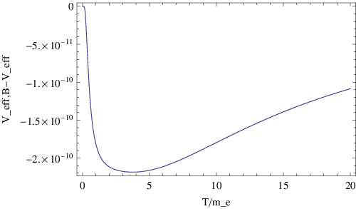
In Fig. 1 we have plotted the potential Eq. (61) as a function of temperature in the range $0$ to 10 MeV for a fixed value of the magnetic field $B=0.1B_{c}$ . This shows that the potential is an increasing function of temperature. We have also shown in Fig. 2, only the magnetic field contribution, i.e. by subtracting the $B=0$ part from Eq. (61), which shows that, the magnetic field contribution is opposite compared to the medium contribution and also order of magnitude smaller.

II.5 Matter Background

Let us consider the background with electrons, positrons, protons, neutrons, neutrinos and anti-neutrinos in the background. As we are considering the magnetic field to be weak, the magnetic field will have no effect on protons and neutrons. For an electron neutrino $\nu_{e}$ propagating in this background, we have

	$\displaystyle a_{W\perp}$	$\displaystyle=$	$\displaystyle-\frac{\sqrt{2}G_{F}}{M_{W}^{2}}\biggl[E_{\nu_{e}}\biggl\{(N_{e}-\bar{N}_{e})-(N_{e}^{0}-\bar{N}_{e}^{0})\biggr\}$		(65)
			$\displaystyle+\frac{m^{4}_{e}}{\pi^{2}}\sum_{l=0}^{\infty}(-1)^{l}\cosh\alpha\biggl\{\left(2-\frac{8}{\sigma^{2}}\right)\frac{K_{1}(\sigma)}{\sigma}-\left(\frac{B}{B_{c}}+\frac{4}{\sigma^{2}}\right)K_{0}(\sigma)\biggr\}\biggr],$		(65)

$\displaystyle b_{e}$	$\displaystyle=$	$\displaystyle b_{W}+b_{Z}+b_{t}=b_{0e}+\tilde{b}_{W}$	(66)
	$\displaystyle=$	$\displaystyle\sqrt{2}G_{F}\biggl[\biggl(1+\frac{3}{2}\frac{m_{e}^{2}}{M_{W}^{2}}+\frac{E_{\nu_{e}}^{2}}{M_{W}^{2}}+C_{V_{e}}\biggr)(N_{e}-\bar{N}_{e})+\biggl(\frac{eB}{M_{W}^{2}}-\frac{E^{2}_{\nu_{e}}}{M_{W}^{2}}\biggr)(N_{e}^{0}-\bar{N}_{e}^{0})$
		$\displaystyle+C_{V_{p}}(N_{p}-\bar{N}_{p})+C_{V_{n}}(N_{n}-\bar{N}_{n})+2(N_{\nu_{e}}-\bar{N}_{\nu_{e}})$
		$\displaystyle+(N_{\nu_{\mu}}-\bar{N}_{\nu_{\mu}})+(N_{\nu_{\tau}}-\bar{N}_{\nu_{\tau}})-\frac{8}{3}\frac{E_{\nu_{e}}}{M_{Z}^{2}}\biggl(\langle E_{\nu_{e}}\rangle N_{\nu_{e}}+\langle\bar{E}_{\nu_{e}}\rangle\bar{N}_{\nu_{e}}\biggr)\biggr]+\tilde{b}_{W},$

and the coefficient of $\hbox to0.0pt{/\hss}b$ is,

	$\displaystyle c_{e}$	$\displaystyle=$	$\displaystyle c_{W}+c_{t}=c_{0e}+\tilde{c}_{W}$		(67)
		$\displaystyle=$	$\displaystyle\sqrt{2}G_{F}\biggl[\biggl(1+\frac{m_{e}^{2}}{2M_{W}^{2}}-\frac{E^{2}_{\nu_{e}}}{M_{W}^{2}}-C_{A_{e}}\biggr)(N_{e}^{0}-\bar{N}_{e}^{0})+\biggl(\frac{eB}{M_{W}^{2}}+\frac{E^{2}_{\nu_{e}}}{M_{W}^{2}}\biggr)(N_{e}-\bar{N}_{e})\biggr]+\tilde{c}_{W},$		(67)

where $\tilde{b}_{W}$ and $\tilde{c}_{W}$ are given in Eqs. (37) and (38). In the weak field limit these two functions are given as

\tilde{b}_{W}=-\sqrt{2}G_{F}\frac{2}{\pi^{2}}\biggl(\frac{m^{2}_{e}}{M_{W}}\biggr)^{2}E_{\nu_{e}}\sum_{l=0}^{\infty}(-1)^{l}\cosh\,\alpha\biggl[\biggl(\frac{6}{\sigma^{2}}-\frac{5}{2}\frac{B}{B_{c}}\biggr)K_{0}(\sigma)+\biggl(3-2\frac{B}{B_{c}}+\frac{12}{\sigma^{2}}\biggr)\frac{K_{1}(\sigma)}{\sigma}\biggr]

(68)

and

\tilde{c}_{W}=\sqrt{2}G_{F}\frac{2}{\pi^{2}}\biggl(\frac{m^{2}_{e}}{M_{W}}\biggr)^{2}E_{\nu_{e}}\sum_{l=0}^{\infty}(-1)^{l}\cosh\,\alpha\biggl[\frac{2}{\sigma^{2}}K_{0}(\sigma)-\biggl(1+2\frac{B}{B_{c}}-\frac{4}{\sigma^{2}}\biggr)\frac{K_{1}(\sigma)}{\sigma}\biggr].

(69)

Similarly for muon and tau neutrinos,

	$\displaystyle b_{\mu}=b_{0\mu}$	$\displaystyle=$	$\displaystyle\sqrt{2}G_{F}\biggl[C_{V_{e}}(N_{e}-\bar{N}_{e})+C_{V_{p}}(N_{p}-\bar{N}_{p})+C_{V_{n}}(N_{n}-\bar{N}_{n})+(N_{\nu_{e}}-\bar{N}_{\nu_{e}})$		(70)
			$\displaystyle+2(N_{\nu_{\mu}}-\bar{N}_{\nu_{\mu}})+(N_{\nu_{\tau}}-\bar{N}_{\nu_{\tau}})-\frac{8}{3}\frac{E_{\nu_{\mu}}}{M_{Z}^{2}}\biggl(\langle E_{\nu_{\mu}}\rangle N_{\nu_{\mu}}+\langle\bar{E}_{\nu_{\mu}}\rangle\bar{N}_{\nu_{\mu}}\biggr)\biggr],$		(70)

and

	$\displaystyle b_{\tau}=b_{0\tau}$	$\displaystyle=$	$\displaystyle\sqrt{2}G_{F}\biggl[C_{V_{e}}(N_{e}-\bar{N}_{e})+C_{V_{p}}(N_{p}-\bar{N}_{p})+C_{V_{n}}(N_{n}-\bar{N}_{n})+(N_{\nu_{e}}-\bar{N}_{\nu_{e}})$		(71)
			$\displaystyle+(N_{\nu_{\mu}}-\bar{N}_{\nu_{\mu}})+2(N_{\nu_{\tau}}-\bar{N}_{\nu_{\tau}})-\frac{8}{3}\frac{E_{\nu_{\tau}}}{M_{Z}^{2}}\biggl(\langle E_{\nu_{\tau}}\rangle N_{\nu_{\tau}}+\langle\bar{E}_{\nu_{\tau}}\rangle\bar{N}_{\nu_{\tau}}\biggr)\biggr].$		(71)

respectively and

	$\displaystyle c_{\mu}$	$\displaystyle=$	$\displaystyle c_{0\mu}=-C_{A_{e}}(N_{e}^{0}-\bar{N}_{e}^{0})$
	$\displaystyle c_{\tau}$	$\displaystyle=$	$\displaystyle c_{0\tau}=-C_{A_{e}}(N_{e}^{0}-\bar{N}_{e}^{0}).$		(72)

For muon and tau neutrinos propagating in the medium $\tilde{c}_{\mu}=\tilde{c}_{\tau}=0$ . The matter potentials experience by different neutrinos for $\phi=0$ are given as

$\displaystyle V_{\nu_{e}}$	$\displaystyle=$	$\displaystyle b_{e}-c_{e}$
$\displaystyle V_{\nu_{\mu}}$	$\displaystyle=$	$\displaystyle b_{\mu}-C_{A_{e}}(N_{e}^{0}-\bar{N}_{e}^{0})$
$\displaystyle V_{\nu_{\tau}}$	$\displaystyle=$	$\displaystyle b_{\tau}-C_{A_{e}}(N_{e}^{0}-\bar{N}_{e}^{0}).$	(73)

Putting the values of $b_{l}$ and $c_{l}$ (for $l=e,\mu,\tau$ ) one can calculate the neutrino potential in the background. For charge neutral matter we should impose

N_{e}-\bar{N}_{e}=N_{p}-\bar{N}_{p},

(74)

and this gives

C_{V_{e}}(N_{e}-\bar{N}_{e})+C_{V_{p}}(N_{p}-\bar{N}_{p})=0,

(75)

in Eqs. (66), (70) and (71). The particle asymmetry is related to the lepton or baryon asymmetry through the relation

L_{a}=\frac{N_{a}-\bar{N}_{a}}{N_{\gamma}},

(76)

where the number density of photon is $N_{\gamma}=\frac{2}{\pi^{2}}\zeta(3)T^{3}$ .

II.6 Only Neutrino Background

In a newly born neutron star, the neutrinos are trapped because the mean free path of these neutrinos are very short compared to the depth of the surrounding medium. So slowly these neutrinos will diffuse out of the region where they are trapped called the neutrino sphere. In the neutrino sphere, the different neutrinos have different average energy, which are given as[41]:

$\displaystyle\langle E_{\nu_{e}}\rangle$	$\displaystyle\simeq$	$\displaystyle 10\,\,MeV$
$\displaystyle\langle\bar{E}_{\nu_{e}}\rangle$	$\displaystyle\simeq$	$\displaystyle 15\,\,MeV$
$\displaystyle\langle\bar{E}_{\nu_{x}}\rangle=\langle E_{\nu_{x}}\rangle$	$\displaystyle\simeq$	$\displaystyle 20\,\,MeV,$	(77)

for $x=\mu,\tau$ . If the medium contains only the neutrinos and anti-neutrinos of all flavors, then for propagating $\nu_{e}$ and $\nu_{\mu}$ we have

	$\displaystyle b_{e}$	$\displaystyle=$	$\displaystyle\sqrt{2}G_{F}\biggl[2(N_{\nu_{e}}-\bar{N}_{\nu_{e}})+(N_{\nu_{\mu}}-\bar{N}_{\nu_{\mu}})+(N_{\nu_{\tau}}-\bar{N}_{\nu_{\tau}})$		(78)
			$\displaystyle-\frac{8}{3}\frac{\langle E_{\nu_{e}}\rangle}{M_{Z}^{2}}\biggl(\langle E_{\nu_{e}}\rangle N_{\nu_{e}}+\langle\bar{E}_{\nu_{e}}\rangle\bar{N}_{\nu_{e}}\biggr)\biggr],$		(78)

and

	$\displaystyle b_{\mu}$	$\displaystyle=$	$\displaystyle\sqrt{2}G_{F}\biggl[(N_{\nu_{e}}-\bar{N}_{\nu_{e}})+2(N_{\nu_{\mu}}-\bar{N}_{\nu_{\mu}})+(N_{\nu_{\tau}}-\bar{N}_{\nu_{\tau}})$		(79)
			$\displaystyle-\frac{8}{3}\frac{1}{M_{Z}^{2}}\biggl(\langle E_{\nu_{\mu}}\rangle^{2}N_{\nu_{\mu}}+\langle\bar{E}_{\nu_{\mu}}\rangle^{2}\bar{N}_{\nu_{\mu}}\biggr)\biggr],$		(79)

respectively and by interchanging $\mu\leftrightarrow\tau$ in Eq. (79) we obtain $b_{\tau}$ for tau neutrino. For only neutrino background we have $c=0$ . As $\langle\bar{E}_{\nu_{x}}\rangle=\langle E_{\nu_{x}}\rangle$ in the neutrino sphere and the propagating neutrinos are also in the background, in Eq. (79) we take $E_{\nu_{x}}=\langle\bar{E}_{\nu_{x}}\rangle=\langle E_{\nu_{x}}\rangle$ . Now the potential difference between $\nu_{e}$ and $\nu_{\mu}$ will be

	$\displaystyle V_{e\mu}$	$\displaystyle=$	$\displaystyle b_{e}-b_{\mu}=\sqrt{2}G_{F}\biggl[(N_{\nu_{e}}-\bar{N}_{\nu_{e}})-(N_{\nu_{\mu}}-\bar{N}_{\nu_{\mu}})$		(80)
			$\displaystyle-\frac{8}{3}\frac{1}{M_{Z}^{2}}\biggl\{\langle E_{\nu_{e}}\rangle\biggl(\langle E_{\nu_{e}}\rangle N_{\nu_{e}}+\langle\bar{E}_{\nu_{e}}\rangle\bar{N}_{\nu_{e}}\biggr)-\biggl(\langle E_{\nu_{\mu}}\rangle^{2}N_{\nu_{\mu}}+\langle{E}_{\nu_{\mu}}\rangle^{2}\bar{N}_{\nu_{\mu}}\biggr)\biggr\}\biggr].$		(80)

Let us assume that the number density of neutrino and anti-neutrino of all flavors are the same inside the neutrino sphere, i.e.

N_{\nu_{l}}=\bar{N}_{\nu_{l}}\,,\,\,\,\,l=e,\mu,\tau,

(81)

and this gives

V_{e\mu}=2.91\times 10^{-18}N_{\nu_{l}}\,MeV^{-2}.

(82)

The potential difference between $\nu_{\mu}$ and $\nu_{\tau}$ vanishes ( $V_{\mu\tau}=0$ ) and the potential difference between $\nu_{e}$ and the sterile neutrino $\nu_{s}$ is given by

V_{es}=b_{e}-b_{s}=-1.32\times 10^{-18}N_{\nu_{l}}\,MeV^{-2}.

(83)

But if we do not take into account the restriction given in Eq. (81) then potential for $\nu_{e}$ , $\nu_{\mu}$ and $\nu_{\tau}$ will different from each other.

III GRB physics and Fireball Model

We have already given a short introduction to GRB and fireball model in sec. 1. As we are interested in the propagation of neutrinos in the fireball medium, let us discuss a bit more about it. The fireball is formed due to the sudden release of huge amount of energy in the form of gamma-rays into a compact region of size $c\delta t$ and it will thermalize with a temperature around 3-10 MeV by producing electron, positron pairs [45]. It will also contaminated by baryons both from the progenitor and the surrounding medium which is believed to be in the range $10^{-8}M_{\odot}-10^{-5}M_{\odot}$ .

Among the GRB community, it is strongly believed that the prompt $\gamma$ which we see in the rage of few 100 keVs to few MeVs for few seconds is due to the synchrotron radiation of charged particles in a magnetic field. But comparatively strong magnetic field is needed to fit the observed data. But it is difficult to estimate the strength of the magnetic field from the first principle. One would expect large magnetic field if the progenitors are highly magnetized, for example, magnetars with $B\sim 10^{16}~G$ . A relatively small pre-existing magnetic field can be amplified due to turbulent dynamo mechanism, compression or shearing. Also under suitable condition the neutrino-electron interaction in the fireball plasma will be able to amplify pre-existing small scale magnetic field. Despite all these, there is no satisfactory explanation for the existence of strong magnetic field in the fireball. Also even if some magnetic flux is carried by the outflow, it will decrease due to the expansion of the fireball at a larger radius. But the strength of the magnetic field will be much smaller than the critical field $B_{C}$ . So the derivation of the effective potential for weak field limit is justified here. However, if we can measure the polarization of the GRBs, it will be helpful to estimate the magnetic field in the fireball as well as give information about the nature of the central engine.

Here we consider a CP-asymmetric $\gamma$ and $e^{-}e^{+}$ fireball, where the excess of electrons come from the electrons associated with the baryons within the fireball. Here for simplicity we assume that the fireball is charge neutral $L_{e}=L_{p}$ and spherical with an initial radius $R\simeq(100-1000)$ km and it has equal number of protons and neutrons. Then the baryon load in the fireball can be given by

	$\displaystyle M_{b}$	$\displaystyle\simeq$	$\displaystyle\frac{16}{3\pi}\xi(3)L_{e}T^{3}R^{3}m_{p}$		(84)
		$\displaystyle\simeq$	$\displaystyle 2.23\times 10^{-4}L_{e}T^{3}_{MeV}R^{3}_{7}M_{\odot}.$		(84)

where $T_{MeV}$ is the fireball temperature expressed in MeV and lies in the range 3-10. The quantity $R_{7}$ is in units of $10^{7}$ cm and $m_{p}$ is the proton mass. For ultra relativistic expansion of the fireball, we assume the baryon load in it to be in the range $10^{-8}M_{\odot}-10^{-5}M_{\odot}$ which corresponds to lepton asymmetry in the range $8.1\times 10^{-4}R^{-3}_{7}\leq L_{e}\leq 8.1\times 10^{-1}R^{-3}_{7}$ .

We have already discussed about the different origins of 5-30 MeV neutrinos. Once these neutrinos are produced, fractions of these neutrinos may propagate through the fireball which is in an extreme condition and may affect the propagation of these neutrinos through it.

IV Three-Neutrino Mixing

To find the neutrino oscillation probabilities, we have to solve the Schroedinger’s equation, given by

i\frac{d\vec{\nu}}{dt}=H\vec{\nu},

(85)

and the state vector in the flavor basis is defined as

\vec{\nu}\equiv(\nu_{e},\nu_{\mu},\nu_{\tau})^{T}.

(86)

The effective Hamiltonian is

H=U\cdot H^{d}_{0}\cdot U^{\dagger}+diag(V_{e},0,0),

(87)

with

H^{d}_{0}=\frac{1}{2E_{\nu}}diag(-\Delta m^{2}_{21},0,\Delta^{2}_{32}).

(88)

Here $V_{e}$ is the charge current (CC) matter potential and $U$ is the three neutrino mixing matrix given by[43, 44]

U={\pmatrix{c_{13}c_{12}&s_{12}c_{13}&s_{13}\cr-s_{12}c_{23}-s_{23}s_{13}c_{12}&c_{23}c_{12}-s_{23}s_{13}s_{12}&s_{23}c_{13}\cr s_{23}s_{12}-s_{13}c_{23}c_{12}&-s_{23}c_{12}-s_{13}s_{12}c_{23}&c_{23}c_{13}\cr}},

(89)

where $s_{ij}=\sin\theta_{ij}$ and $c_{ij}=\cos\theta_{ij}$ . For anti-neutrinos one has to replace $(N_{a}-{\bar{N}}_{a})$ by $-(N_{a}-{\bar{N}}_{a})$ and $U$ by $U^{*}$ . The higher order contribution to potential does not change the sign. Here we have to emphasize that the neutral current (NC) contribution is not taken into account. This is because in the matter background the NC contribution to all the neutrinos is the same and when we take the difference of potential, this contribution will be cancelled out and does not affect the neutrino oscillation. But it has to be remembered that, in the neutrino background where $N_{\nu}-{\bar{N}}_{\nu}\neq 0$ , the potential for different neutrinos are different which described in Sec.II.6 and in this case we can not neglect the NC contribution. The different neutrino probabilities are given as

$\displaystyle P_{ee}$	$\displaystyle=$	$\displaystyle 1-4s^{2}_{13,m}c^{2}_{13,m}S_{31},$
$\displaystyle P_{\mu\mu}$	$\displaystyle=$	$\displaystyle 1-4s^{2}_{13,m}c^{2}_{13,m}s^{4}_{23}S_{31}-4s^{2}_{13,m}s^{2}_{23}c^{2}_{23}S_{21}-4c^{2}_{13,m}s^{2}_{23}c^{2}_{23}S_{32},$
$\displaystyle P_{\tau\tau}$	$\displaystyle=$	$\displaystyle 1-4s^{2}_{13,m}c^{2}_{13,m}c^{4}_{23}S_{31}-4s^{2}_{13,m}s^{2}_{23}c^{2}_{23}S_{21}-4c^{2}_{13,m}s^{2}_{23}c^{2}_{23}S_{32},$
$\displaystyle P_{e\mu}$	$\displaystyle=$	$\displaystyle 4s^{2}_{13,m}c^{2}_{13,m}s^{2}_{23}S_{31},$
$\displaystyle P_{e\tau}$	$\displaystyle=$	$\displaystyle 4s^{2}_{13,m}c^{2}_{13,m}c^{2}_{23}S_{31}$
$\displaystyle P_{\mu\tau}$	$\displaystyle=$	$\displaystyle-4s^{2}_{13,m}c^{2}_{13,m}s^{2}_{23}c^{2}_{23}S_{31}+4s^{2}_{13,m}s^{2}_{23}c^{2}_{23}S_{21}+4c^{2}_{13,m}s^{2}_{23}c^{2}_{23}S_{32},$

where

\sin 2\theta_{13,m}=\frac{\sin 2\theta_{13}}{\sqrt{(\cos 2\theta_{13}-2E_{\nu}V_{e}/\Delta m^{2}_{32})^{2}+(\sin 2\theta_{13})^{2}}},

(91)

and

S_{ij}=\sin^{2}\biggl(\frac{\Delta\mu^{2}_{ij}}{4E_{\nu}}L\biggr).

(92)

$\displaystyle\Delta\mu^{2}_{21}$	$\displaystyle=$	$\displaystyle\frac{\Delta m^{2}_{32}}{2}\biggl(\frac{\sin 2\theta_{13}}{\sin 2\theta_{13,m}}-1\biggr)-E_{\nu}V_{e}$
$\displaystyle\Delta\mu^{2}_{32}$	$\displaystyle=$	$\displaystyle\frac{\Delta m^{2}_{32}}{2}\biggl(\frac{\sin 2\theta_{13}}{\sin 2\theta_{13,m}}+1\biggr)+E_{\nu}V_{e}$
$\displaystyle\Delta\mu^{2}_{31}$	$\displaystyle=$	$\displaystyle\Delta m^{2}_{32}\frac{\sin 2\theta_{13}}{\sin 2\theta_{13,m}}$	(93)

where

	$\displaystyle\sin^{2}\theta_{13,m}$	$\displaystyle=$	$\displaystyle\frac{1}{2}\biggl(1-\sqrt{1-\sin^{2}2\theta_{13,m}}\biggr)$
	$\displaystyle\cos^{2}\theta_{13,m}$	$\displaystyle=$	$\displaystyle\frac{1}{2}\biggl(1+\sqrt{1-\sin^{2}2\theta_{13,m}}\biggr)$		(94)

The oscillation length for the neutrino is given by

L_{osc}=\frac{L_{v}}{\sqrt{\cos^{2}2\theta_{13}(1-\frac{2E_{\nu}V_{e}}{\Delta m^{2}_{32}\cos 2\theta_{13}})^{2}+\sin^{2}2\theta_{13}}},

(95)

where $L_{v}=4\pi E_{\nu}/\Delta m^{2}_{32}$ is the vacuum oscillation length. For resonance to occur, we should have $V_{eff,B}=V_{e}>0$ and

\cos 2\theta_{13}=\frac{2E_{\nu}V_{e}}{\Delta m^{2}_{32}}.

(96)

By putting $V_{e}$ and simplifying we obtain

\Phi_{A}-1.58027\times 10^{-10}E_{\nu,MeV}\Phi_{B}\simeq 2.24208\frac{\tilde{\Delta}m^{2}_{32}}{E_{\nu,MeV}}\cos 2\theta_{13},

(97)

Table 1: We have shown the different observables of the fireball as well as the neutrino resonance length

L_{res}

for

\Delta m^{2}_{23}=10^{-2.9}eV^{2}

and

B=0.1B_{c}

$E_{\nu,MeV}$	T(MeV)	$\mu(eV)$	$L_{e}$	$L_{res}(cm)$	$M_{b}(R^{3}_{7}M_{\odot})$
5	3	$2.47412$	$1.099\times 10^{-6}$	$4.737\times 10^{6}$	$7.064\times 10^{-9}$
	10	$0.960329$	$1.284\times 10^{-7}$		$3.057\times 10^{-8}$
10	3	$1.33789$	$5.943\times 10^{-7}$	$9.474\times 10^{6}$	$3.819\times 10^{-9}$
	10	$1.59669$	$2.135\times 10^{-7}$		$5.083\times 10^{-8}$
20	3	$0.869801$	$3.864\times 10^{-7}$	$1.895\times 10^{7}$	$2.483\times 10^{-9}$
	10	$3.03194$	$4.055\times 10^{-7}$		$9.653\times 10^{-8}$
30	3	$0.804489$	$3.574\times 10^{-7}$	$2.842\times 10^{7}$	$2.297\times 10^{-9}$
	10	$4.50277$	$6.022\times 10^{-7}$		$1.434\times 10^{-7}$

Table 2: We have shown the different observables of the fireball as well as the neutrino resonance length

L_{res}

for

\Delta m^{2}_{23}=10^{-2.2}eV^{2}

and

B=0.1B_{c}

$E_{\nu,MeV}$	T(MeV)	$\mu(eV)$	$L_{e}$	$L_{res}(cm)$	$M_{b}(R^{3}_{7}M_{\odot})$
5	3	$12.1177$	$5.383\times 10^{-6}$	$9.452\times 10^{5}$	$3.460\times 10^{-8}$
	10	$1.82987$	$2.447\times 10^{-7}$		$5.826\times 10^{-8}$
10	3	$6.17192$	$2.742\times 10^{-6}$	$1.890\times 10^{6}$	$1.762\times 10^{-8}$
	10	$2.03432$	$2.721\times 10^{-7}$		$6.477\times 10^{-8}$
20	3	$3.27657$	$1.456\times 10^{-6}$	$3.780\times 10^{6}$	$9.355\times 10^{-9}$
	10	$3.24878$	$4.346\times 10^{-7}$		$1.034\times 10^{-7}$
30	3	$2.4178$	$1.074\times 10^{-6}$	$5.671\times 10^{6}$	$6.903\times 10^{-9}$
	10	$4.6475$	$6.216\times 10^{-7}$		$1.480\times 10^{-7}$

where ${\tilde{\Delta}m^{2}_{32}}$ is expressed in $eV^{2}$ and $E_{\nu,MeV}$ is in MeV. The functions $\Phi_{A}$ and $\Phi_{B}$ are defined in Eqs. (63) and (64). Now we have to evaluate the above condition for given values of ${\tilde{\Delta}m^{2}_{32}}$ and $\cos 2\theta_{13}$ from experiments and different values of temperature (T) and chemical potential ( $\mu$ ). At resonance, the oscillation length becomes the resonance length and can be given by

L_{res}=\frac{L_{v}}{\sin 2\theta_{13}}.

(98)

So far we have assumed that the neutrino potential does not vary with distance. However $V_{eff,B}$ will vary with distance. So we have to consider the adiabatic condition at the resonance, which can be given by

	$\displaystyle\kappa_{res}$	$\displaystyle\equiv$	$\displaystyle\frac{2}{\pi}\left(\frac{\Delta m^{2}_{32}}{2E_{\nu}}\sin 2\theta_{13}\right)^{2}\left(\frac{dV_{eff,B}}{dr}\right)^{-1}\geq 1$		(99)
		$\displaystyle=$	$\displaystyle 3.62\times 10^{-2}\left(\frac{{\tilde{\Delta}m}^{2}_{32}}{E_{\nu,MeV}}\sin 2\theta_{13}\right)^{2}\frac{l_{cm}}{\Phi^{\prime}}\geq 1,$		(99)

where

\Phi^{\prime}=\frac{d\Phi_{A}}{dx}-1.58027\times 10^{-10}E_{\nu,MeV}\frac{d\Phi_{B}}{dx}.

(100)

In the above equations we have expressed $l_{cm}$ in centimeter and $x$ is a dimensionless variable.

V Results

We have done a complete analysis for three neutrino mixing with and without magnetic field. For our analysis we have used the result given in ref.[43],

	$\displaystyle 1.4\times 10^{-3}<\Delta m^{2}_{32}/eV^{2}<6.0\times 10^{-3}$
	$\displaystyle\theta_{13}\simeq 6^{\circ}$
	$\displaystyle 32^{\circ}<\theta_{23}<60^{\circ}.$		(101)

The above result is obtained by performing a global analysis and taking full set of data from solar, atmospheric and reactor experiments. In the above we consider $\theta_{23}=45^{\circ}$ .

Different values of $\mu$ and $T$ are shown in Fig. 3 for which the resonance condition in Eq. (97) is satisfied. We have used two extreme values of $\Delta m^{2}_{32}$ i.e. $10^{-2.9}\,eV^{2}$ in Fig. 3a and $10^{-2.21}\,eV^{2}$ in Fig. 3b for $B=0.1B_{c}$ , $\theta_{13}=6^{\circ}$ and four different neutrino energies $5$ , $10$ , $20$ and $30$ MeV respectively. In both small and large values of $\Delta m^{2}_{32}$ and fireball temperature in the range $3$ to $10$ MeV, the chemical potential of the electron is in the 1-12 eV range which are shown in Table I and II. In Table I we have shown the different fireball observables for $\Delta m^{2}_{32}=10^{-2.9}\,eV^{2}$ . It shows that going from neutrino energy 5 MeV to 30 MeV, the resonance length changes between 47 km to 284 km and lepton asymmetry $~\sim 10^{-7}$ to $~10^{-6}$ . For a charge neutral plasma $L_{e}=L_{p}$ this translates to a baryon load in the fireball in the range $2.3\times 10^{-9}M_{\odot}<M_{b}<1.4\times 10^{-7}M_{\odot}$ . In Table II we have done the same analysis but for $\Delta m^{2}_{32}=10^{-2.2}\,eV^{2}$ . Here the chemical potential is higher compared to the one in Table I. This shows that shift in $\Delta m^{2}_{32}$ towards higher value also shift the $\mu$ in the same direction. In this case there is not much change in $L_{e}$ and $M_{b}$ and the resonance length lies in the range $9.4\,km<L_{res}<57\,km$ .

The above analysis of the resonance condition shows that, in the temperature range of 3 to 10 MeV, the resonance condition is satisfied for electron chemical potential ( $\mu$ ) between 1 to 12 eV. Also for neutrino energy in the range 5 to 30 MeV, the resonance length lies below 284 km, which shows that neutrinos can resonantly oscillate within the fireball of radius 100 to 1000 km. The baryon load of the fireball also lies in the range $10^{-9}M_{\odot}<M_{b}<10^{-7}M_{\odot}$ . If the potential has a profile that means, the functions $\Phi_{A}$ and $\Phi_{B}$ depend on the length scale then we found that for $10^{-2.9}\,eV^{2}\leq\Delta m^{2}_{32}\leq 10^{-2.2}\,eV^{2}$ and $5\leq E_{\nu,MeV}\leq 30$ , the parameter $l_{cm}/{\Phi^{\prime}}$ will lie in the range $10^{-10}$ to $2.5\times 10^{-9}$ to satisfy the condition given in Eq. (99).

The survival and conversion probabilities for the active neutrinos are plotted as function of $\Delta m^{2}_{32}$ in the range $10^{-2.9}~eV^{2}$ to $10^{-2.2}~eV^{2}$ for $B=0$ and $B=0.1B_{c}$ for two neutrino energies 5 MeV and 30 MeV from Fig. 4 to Fig. 7. We have also considered two different length scales for the fireball i.e. 100 km and 1000 km to see how the probabilities changes when the length scale of the fireball changes. As we are taking $\theta_{23}=45^{\circ}$ , the probabilities $P_{e\mu}=P_{e\tau}$ and also $P_{\mu\mu}=P_{\tau\tau}$ .

We have plotted the survival probability of muon neutrino for $L=100\,km$ in Fig. 4a and for $L=1000\,km$ in Fig. 4b. The survival probability of muon $P_{\mu\mu}$ neutrino in Fig. 3a, for neutrino energy 5 MeV and magnetic field $B=0$ is $180^{\circ}$ out of phase compared to the same neutrino energy but for $B=0.1B_{c}$ . For $B=0$ case the probability varies between $0.6$ and unity and for $B=0.1B_{c}$ it is between $0$ and $0.4$ . Going from 5 MeV to 30 MeV we saw that, for $B=0$ ,the $P_{\mu\mu}$ decreases and lies between $0.3$ and $0.5$ and for $B=0.1B_{c}$ lies between $0.42$ and $0.68$ . Going from $L=100\,km$ to $L=1000\,km$ (Fig. 4b), we see that both $B=0$ and $B=0.1B_{c}$ have a small phase difference and the $P_{\mu\mu}$ varies between $0$ and $1$ . But $P_{\mu\mu}$ for $B=0.1B_{c}$ lags behind the one for $B=0$ for both neutrino energies 5 MeV and 30 MeV. The probability for low energy (5 MeV curve) neutrino oscillates faster than the one for 30 MeV.

In Fig. 5, we have plotted the conversion probability $P_{e\mu}$ for $E_{\nu}=5\,MeV$ , $L=100\,km$ (5a) and $E_{\nu}=5\,MeV$ , $L=1000\,km$ (5b) respectively for both $B=0$ and $B=0.1B_{c}$ . It shows that in Fig. 5a, the $P_{e\mu}$ for $B=0$ and $B=0.1B_{c}$ are having the same phase difference of $180^{\circ}$ as in Fig. 4a. But the probability is very small $\sim 10^{-9}$ . Going from Fig. 5a to 5b ( $L=1000\,km$ ) , we saw that the phase difference is almost gone away and $P_{e\mu}$ oscillates much faster compared to the one in Fig 5a.

In Figs. 6a and 6b, we have the same probability $P_{e\mu}$ as in Fig. 5, but here the neutrino energy $E_{\nu}=30\,MeV$ . It is clearly seen in Fig. 6a that both the probabilities are out of phase and are very small $\sim 10^{-10}$ . On the other hand for $L=1000\,km$ (Fig. 6b) the phase difference is gone and the $P_{e\mu}$ oscillates much faster than the one in Fig. 6a. We have the $P_{e\mu}=P_{e\tau}\simeq 10^{-10}$ which gives $P_{ee}\simeq 1$ . This shows that the electron neutrinos propagating within the fireball can not oscillate to other neutrinos.

In Fig. 7a and 7b we have plotted the $P_{\mu\tau}$ for $L=100\,km$ and $L=1000\,km$ respectively. For $L=100\,km$ the probability for $B=0$ and $B=0.1B_{c}$ are out of phase for both $E_{\nu}=5$ and $30MeV$ in Fig 7a. In Fig. 7b for $L=1000\,km$ there is a small phase difference between the $B=0$ and $B=0.1B_{c}$ probabilities. Comparison of Fig. 4a with Fig. 7a and Fig. 4b with Fig. 7b show that the $B=0$ probability (in Fig. 4a and Fig. 7a) and $B=0.1B_{c}$ probability (in Fig. 4b and Fig. 7b) are $180^{\circ}$ out of phase. We obtain this because the probability satisfies the condition

P_{\mu\mu}+P_{e\mu}+P_{\mu\tau}=1.

(102)

We have shown in Figs. 5 and 6 that $P_{e\mu}=P_{e\tau}$ and they are very small which gives $P_{\mu\tau}\simeq 1-P_{\mu\mu}$ . The $P_{\tau\tau}$ is same as $P_{\mu\mu}$ .

From our analysis we see that $P_{ee}\simeq 1$ and is almost independent of the energy of the neutrinos and the size of the fireball, which shows that for small mixing corresponding to $\theta_{13}=6^{\circ}$ and for $\theta_{23}=45^{\circ}$ , the electron neutrino almost does not oscillate to any other flavor which is obvious from the Fig. 5 and Fig. 6. On the other hand, the muon and tau neutrinos oscillate among themselves with equal probability and the oscillation depends on the neutrino energy, magnetic field and size of the fireball. Comparison of $B=0$ and $B\neq 0$ results show that the magnetic field contribution is order of magnitude smaller than the medium case. But depending on the size of the fireball, the probability for $B=0$ and $B\neq 0$ are either in phase or out of phase.

VI conclusions

We have shown that neutrino self-energy in the presence of a magnetic field can also be expressed as

{\tilde{\Sigma}}=a_{\perp}\hbox to0.0pt{/\hss}k_{\perp}+b\hbox to0.0pt{/\hss}u+c\hbox to0.0pt{/\hss}b,\\

by absorbing the ${\hbox to0.0pt{/\hss}k}_{\parallel}$ component with the two four vectors ${\hbox to0.0pt{/\hss}u}$ and ${\hbox to0.0pt{/\hss}b}$ . The above decomposition is only valid when the magnetic field is along the z-axis. In addition to this we have also shown that the neutrino effective potential $V_{eff,B}$ is independent of how we decompose the the self-energy in terms of Lorentz scalars as shown in Eqs. (1) and (VI). We have explicitly calculated the $V_{eff,B}$ up to order $M^{-4}_{W}$ in the weak field limit $eB\ll m^{2}_{e}$ in terms of Bessel Functions and recover the result for $B=0$ limit which can only be obtained when $k_{3}$ the third component of the neutrino momentum is replaced by $-E_{\nu}$ . We have also calculated the neutrino effective potential when the background contains (i) $e^{-},e^{+}$ , protons, neutrons and neutrinos and (ii) only neutrinos in the background. By considering the three-neutrino mixing we have studied the active-active neutrino oscillation process $\nu_{a}\leftrightarrow\nu_{b}$ ( $a$ and $b$ are active) in the weakly magnetized $e^{-}e^{+}$ , $p$ and $n$ plasma of the GRB fireball assuming it to be spherical with a radius of 100 to 1000 km and temperature in the range 3-10 MeV. We further assume that the fireball is charge neutral due to the presence of protons and their accompanying electrons. The baryon load of the fireball is solely due to the presence of almost equal number of protons and neutrons in it.

Our analysis shows that the $\nu_{e}$ almost does not oscillate to any other flavors and $P_{ee}\simeq 1$ is independent of the $\nu_{e}$ energy as well as the background magnetic field. The non oscillation of $\nu_{e}$ to other flavors gives $P_{e\mu}$ and $P_{e\tau}$ very small of the order of $10^{-10}$ . But the $\nu_{\mu}$ and $\nu_{\tau}$ oscillate among themselves, which depends on the energy of the neutrino, magnetic field and also on the size of the fireball. We analyzed our result by taking two different radius of the fireball i.e. 100 km and 1000 km, neutrino energy in the range 5 to 30 MeV and magnetic field $B=0$ and $B=0.1B_{c}$ with $B_{c}=4.14\times 10^{13}$ Gauss. We found that the probability for $B=0$ and $B=0.1B_{c}$ are out of phase by $180^{\circ}$ for $L=100$ km and almost in phase for $L=1000$ km. For $L=100$ km, the $P_{\mu\mu}$ and $P_{\mu\tau}$ do vary between 0-0.5 or 0.5-1. On the other hand for $L=1000$ km, it varies between 0 and 1. Also in this case low energy neutrinos oscillate faster than the high energy one.

We have also analyzed the resonance condition and found that, to satisfy the resonance condition, the electron chemical potential in the fireball lies in the range 1-12 eV. For neutrino energy in the range 5 to 30 MeV the resonance length lies in the range 9.4 km to 284 km. So if we consider a fireball of 100 km to 1000 km radius this shows that the resonant oscillation of $\nu_{\mu}$ and $\nu_{\tau}$ neutrinos can take place but not the $\nu_{e}$ . The baryon load calculated by using the resonance condition lies in the range $10^{-9}M_{\odot}<M_{b}<10^{-7}M_{\odot}$ . Depending on the size of the fireball the probability for $B=0$ and $B\neq 0$ are either in phase or out of phase.

ACKNOWLEDGMENTS
We are thankful to B. Zhang and S. Nagataki for many useful discussions. Y.Y. K and S. S. thank APCTP for the kind hospitality during their several visits, where this work has been initiated. The Work of S. S. is partially supported by DGAPA-UNAM (Mexico) project IN101409, Y.Y.K’s work is partially supported by APCTP in Korea and is supported in part by National Research Foundation of Korea Grant funded by the Korean Government 2009-0070667.

References

[1] P. Elmfors, D. Grasso and G. Raffelt, Nucl. Phys. B 479, 3 (1996) [arXiv:hep-ph/9605250].
[2] H. B. J. Koers and R. A. M. Wijers, Mon. Not. Roy. Astron. Soc. 364, 934 (2005) [arXiv:astro-ph/0505533].
[3] L. Dessart, C. Ott, A. Burrows, S. Rosswog and E. Livne, arXiv:0806.4380 [astro-ph].
[4] S. Sahu, N. Fraija and Y. Y. Keum, Phys. Rev. D 80, 033009 (2009) [arXiv:0904.0138 [hep-ph]].
[5] P. Langacker, J. P. Leveille and J. Sheiman, Phys. Rev. D 27, 1228 (1983).
[6] A. Bravo Garcia, K. Bhattacharya and S. Sahu, Mod. Phys. Lett. A 23, 2771 (2008) [arXiv:0706.3921 [hep-ph]].
[7] T. Piran, Phys. Rept. 314 (1999) 575 [arXiv:astro-ph/9810256].
[8] C. A. Meegan et al., Nature 355, 143 (1992).
[9] B. Zhang and P. Meszaros, Int. J. Mod. Phys. A 19, 2385 (2004) [arXiv:astro-ph/0311321].
[10] T. Piran, Phys. Rept. 333, 529 (2000) [arXiv:astro-ph/9907392].
[11] M. Della Valle, Nuovo Cim. 28C, 563 (2005) [arXiv:astro-ph/0504517].
[12] N. Gehrels et al., Nature 437, 851 (2005) [arXiv:astro-ph/0505630].
[13] S. D. Barthelmy et al., Nature 438, 994 (2005) [arXiv:astro-ph/0511579].
[14] J. S. Villasenor et al., Nature 437, 855 (2005) [arXiv:astro-ph/0510190].
[15] J. Hjorth et al., Nature 437, 859 (2005) [arXiv:astro-ph/0510096].
[16] E. Berger et al., Nature 438, 988 (2005) [arXiv:astro-ph/0508115].
[17] V. V. Usov, Nature 357, 472 (1992).
[18] D. A. Uzdensky and A. I. MacFadyen, Phys. Plasmas 14, 056506 (2007) [arXiv:0707.0576 [astro-ph]].
[19] I.H. Park et al.(UFFO collaboration), The UFFO(Ultra-Fast Flash Observatory) Pathfinder: Proposed Space Mission for Lomonosov Spacecraft.
[20] E. Waxman, Lect. Notes Phys. 598 (2003) 393 [arXiv:astro-ph/0303517].
[21] J. Goodman, Astrophys. J. 308 (1986) L47.
[22] G. Vedrenne and J. Atteia, “Gamma-Ray Bursts: The brighest Explotions in the Universe,” Springer, Praxis Publishing Ltd, Chichester, UK, 2009
[23] W. H. Lee and E. Ramirez-Ruiz, New J. Phys. 9, 17 (2007) [arXiv:astro-ph/0701874].
[24] G. G. Raffelt, Astrophys. J. 561, 890 (2001) [arXiv:astro-ph/0105250].
[25] M. Ruffert and H. T. Janka, Astron. Astrophys. 344, 573 (1999) [arXiv:astro-ph/9809280].
[26] J. Goodman, A. Dar and S. Nussinov, Astrophys. J. 314 (1987) L7.
[27] E. Waxman and J. N. Bahcall, Phys. Rev. Lett. 78, 2292 (1997) [arXiv:astro-ph/9701231].
[28] R. R. Volkas and Y. Y. Y. Wong, Astropart. Phys. 13, 21 (2000) [arXiv:astro-ph/9907161].
[29] B. Dasgupta, A. Dighe, A. Mirizzi and G. G. Raffelt, Phys. Rev. D 78, 033014 (2008) [arXiv:0805.3300 [hep-ph]].
[30] H. Nunokawa, V. B. Semikoz, A. Y. Smirnov and J. W. F. Valle, [arXiv:hep-ph/9701420].
[31] J. F. Nieves, Phys. Rev. D 42, 4123 (1990) [Erratum-ibid. D 49, 3067 (1994)].
[32] H. A. Weldon, Phys. Rev. D 26, 1394 (1982).
[33] J. C. D’Olivo, J. F. Nieves and S. Sahu, Phys. Rev. D 67, 025018 (2003) [arXiv:hep-ph/0208146].
[34] A. Erdas and G. Feldman, Nucl. Phys. B 343, 597 (1990).
[35] J. Schwinger Phys. Rev. Lett.82, 5, 664, (1951)
[36] K. Enqvist, K. Kainulainen and J. Maalampi, Nucl. Phys. B 349, 754 (1991).
[37] S. Sahu and V. M. Bannur, Phys. Rev. D 61, 023003 (2000) [arXiv:hep-ph/9806427].
[38] S. Sahu and J. C. D’Olivo, Phys. Rev. D 71, 047303 (2005) [arXiv:hep-ph/0502043].
[39] A. Erdas, C. W. Kim and T. H. Lee, Phys. Rev. D 58, 085016 (1998) [arXiv:hep-ph/9804318].
[40] A. Bravo. Garcia and S. Sahu, Mod. Phys. Lett. A 22 (2007) 213.
[41] C. Giunti and C. W. Kim, Fundamentals of Neutrino Physics and Astrophysics, Oxford Univ.Press, pg 525 (2007)
[42] P. Meszaros, Nucl. Phys. Proc. Suppl. 80, 63 (2000) [arXiv:astro-ph/9904038].
[43] M. C. Gonzalez-Garcia and Y. Nir, Rev. Mod. Phys. 75, 345 (2003) [arXiv:hep-ph/0202058].
[44] E. K. Akhmedov, R. Johansson, M. Lindner, T. Ohlsson and T. Schwetz, JHEP 0404, 078 (2004) [arXiv:hep-ph/0402175].
[45] B. Zhang and P. Meszaros, Astrophys. J. 566, 712 (2002) [arXiv:astro-ph/0108402].

Propagation of Neutrinos through Magnetized Gamma-Ray Burst Fireball

Abstract

pacs

I Introduction

II Neutrino Effective Potential

II.1 Neutrino self-energy

II.2 Weak field limit e​B≪me2eB\ll m^{2}_{e}

II.3 Neutrino Potential without Magnetic field

II.4 Comparison of Ve​f​fV_{eff} with and without magnetic field

II.5 Matter Background

II.6 Only Neutrino Background

III GRB physics and Fireball Model

IV Three-Neutrino Mixing

V Results

VI conclusions

References

II.2 Weak field limit $eB\ll m^{2}_{e}$

II.4 Comparison of $V_{eff}$ with and without magnetic field