Behavior of $F(R)$ gravity around a crossing of the phantom divide

Kazuharu Bamba Note: E-mail address: bamba@phys.nthu.edu.tw Affiliation: Department of Physics, National Tsing Hua University, Hsinchu, Taiwan 300

Abstract

We study a model of $F(R)$ gravity in which a crossing of the phantom divide can be realized. In particular, we demonstrate the behavior of $F(R)$ gravity around a crossing of the phantom divide by taking into account the presence of cold dark matter.

pacs

04.50.Kd, 95.36.+x, 98.80.-k

I Introduction

It is observationally supported that the current expansion of the universe is accelerating [1, 2]. The scenarios to account for the current accelerated expansion of the universe fall into two broad categories [3, 4, 5, 6, 7, 8, 9, 10, 11]. One is to introduce “dark energy” in the framework of general relativity. The other is to study a modified gravitational theory, e.g., $F(R)$ gravity, in which the action is represented by an arbitrary function $F(R)$ of the scalar curvature $R$ (for reviews, see [6, 7, 8, 9, 10, 11]; and for a new approach, see [12]).

On the other hand, various observational data [13] imply that the ratio of the effective pressure to the effective energy density of the universe, i.e., the effective equation of state (EoS) $w_{\mathrm{eff}}\equiv p_{\mathrm{eff}}/\rho_{\mathrm{eff}}$ , may evolve from larger than $-1$ (non-phantom phase) to less than $-1$ (phantom phase [14, 15]). Namely, it crosses $-1$ (the phantom divide) at the present time or in the near past. A number of models to realize the crossing of the phantom divide have been proposed (for a detailed review, see [4]).

There are also several studies for the crossing of the phantom divide in the framework of $F(R)$ gravity [6, 17, 16, 18, 19, 20, 21, 22]¹¹ 1 The equivalence between $F(R)$ gravity and the scalar-tensor theory has been indicated in Ref. [23]. The crossing of the phantom divide in scalar-tensor theories has been investigated in Ref. [24]. (for related works, see [25]). An explicit model with realizing a crossing of the phantom divide has been constructed in Ref. [26] and its thermodynamics has been examined [27]. Moreover, in Ref. [28] it has been illustrated that multiple crossings of the phantom divide can occur in $F(R)$ gravity as the scalar field theories such as an oscillating quintom model [29] or a quintom with two scalar fields [30] in the framework of general relativity (see also [31, 32]).

In this paper, we study a model of $F(R)$ gravity in which a crossing of the phantom divide can be realized by taking into account the presence of cold dark matter. We demonstrate the behavior of $F(R)$ gravity around a crossing of the phantom divide. In our previous work [26], an analytic solution of $F(R)$ gravity to realize a crossing of the phantom divide without matter has been derived. In this work, as a further investigation, we examine a solution of $F(R)$ gravity to realize a crossing of the phantom divide with cold dark matter. We use units of $k_{\mathrm{B}}=c=\hbar=1$ and denote the gravitational constant $8\pi G$ by ${\kappa}^{2}\equiv 8\pi/{M_{\mathrm{Pl}}}^{2}$ with the Planck mass of $M_{\mathrm{Pl}}=G^{-1/2}=1.2\times 10^{19}$ GeV.

The paper is organized as follows. In Sec. II, we explain the reconstruction method of $F(R)$ gravity proposed in Ref. [33]. In Sec. III, we study a model of $F(R)$ with realizing a crossing of the phantom divide by using the reconstruction method and investigate the behavior of $F(R)$ gravity around a crossing of the phantom divide. Finally, conclusions are given in Sec. IV.

II Reconstruction method

First, we explain the reconstruction method of $F(R)$ gravity proposed in Ref. [33]. The action of $F(R)$ gravity with matter is as follows:

\displaystyle S=\int d^{4}x\sqrt{-g}\left[\frac{F(R)}{2\kappa^{2}}+{\mathcal{L}}_{\mathrm{matter}}\right]\,,

(1)

where $g$ is the determinant of the metric tensor $g_{\mu\nu}$ and ${\mathcal{L}}_{\mathrm{matter}}$ is the matter Lagrangian. By using proper functions $P(\phi)$ and $Q(\phi)$ of a scalar field $\phi$ , the action in Eq. (1) can be rewritten to

\displaystyle S=\int d^{4}x\sqrt{-g}\left\{\frac{1}{2\kappa^{2}}\left[P(\phi)R+Q(\phi)\right]+{\mathcal{L}}_{\mathrm{matter}}\right\}\,.

(2)

The scalar field $\phi$ may be regarded as an auxiliary scalar field because it has no kinetic term. From Eq. (1), the equation of motion of $\phi$ is given by

\displaystyle 0=\frac{dP(\phi)}{d\phi}R+\frac{dQ(\phi)}{d\phi}\,.

(3)

Substituting $\phi=\phi(R)$ into the action in Eq. (2) yields the expression of $F(R)$ as

\displaystyle F(R)=P(\phi(R))R+Q(\phi(R))\,.

(4)

From Eq. (2), the field equation of modified gravity is derived as

\displaystyle\frac{1}{2}g_{\mu\nu}\left[P(\phi)R+Q(\phi)\right]-R_{\mu\nu}P(\phi)-g_{\mu\nu}\Box P(\phi)+{\nabla}_{\mu}{\nabla}_{\nu}P(\phi)+\kappa^{2}T^{(\mathrm{matter})}_{\mu\nu}=0\,,

(5)

where ${\nabla}_{\mu}$ is the covariant derivative operator associated with $g_{\mu\nu}$ , $\Box\equiv g^{\mu\nu}{\nabla}_{\mu}{\nabla}_{\nu}$ is the covariant d’Alembertian for a scalar field, and $T^{(\mathrm{matter})}_{\mu\nu}$ is the contribution to the energy-momentum tensor form matter.

We assume the flat Friedmann-Robertson-Walker (FRW) space-time with the metric,

\displaystyle{ds}^{2}=-{dt}^{2}+a^{2}(t)d{\mbox{\boldmath$x$}}^{2}\,,

(6)

where $a(t)$ is the scale factor. In this background, the components of $(\mu,\nu)=(0,0)$ and $(\mu,\nu)=(i,j)$ $(i,j=1,\cdots,3)$ in Eq. (5) read

	$\displaystyle-6H^{2}P(\phi(t))-Q(\phi(t))-6H\frac{dP(\phi(t))}{dt}+2\kappa^{2}\rho=0\,,$		(7)
	$\displaystyle 2\frac{d^{2}P(\phi(t))}{dt^{2}}+4H\frac{dP(\phi(t))}{dt}+\left(4\dot{H}+6H^{2}\right)P(\phi(t))+Q(\phi(t))+2\kappa^{2}p=0\,,$		(8)

where $H=\dot{a}/a$ is the Hubble parameter with $\dot{~}=\partial/\partial t$ and $\rho$ and $p$ are the sum of the energy density and pressure of matters with a constant EoS $w_{i}$ , respectively, with $i$ being some component of matters. After eliminating $Q(\phi)$ from Eqs. (7) and (8), we get

\displaystyle\frac{d^{2}P(\phi(t))}{dt^{2}}-H\frac{dP(\phi(t))}{dt}+2\dot{H}P(\phi(t))+\kappa^{2}\left(\rho+p\right)=0\,.

(9)

The scalar field $\phi$ may be taken as $\phi=t$ if it is redefined properly. By representing $a(t)$ as

\displaystyle a(t)=\bar{a}\exp\left(\tilde{g}(t)\right)

(10)

in terms of a constant of $\bar{a}$ and a proper function of $\tilde{g}(t)$ and using $H=d\tilde{g}(\phi)/\left(d\phi\right)$ , we rewrite Eq. (9) to be

	$\displaystyle\frac{d^{2}P(\phi)}{d\phi^{2}}-\frac{d\tilde{g}(\phi)}{d\phi}\frac{dP(\phi)}{d\phi}+2\frac{d^{2}\tilde{g}(\phi)}{d\phi^{2}}P(\phi)$
	$\displaystyle\hskip 28.45274pt{}+\kappa^{2}\sum_{i}\left(1+w_{i}\right)\bar{\rho}_{i}\bar{a}^{-3\left(1+w_{i}\right)}\exp\left[-3\left(1+w_{i}\right)\tilde{g}(\phi)\right]=0\,,$		(11)

where $\bar{\rho}_{i}$ is a constant. Moreover, from Eq. (7), we obtain

	$\displaystyle Q(\phi)$	$\displaystyle\hskip-1.99997pt=\hskip-1.99997pt$	$\displaystyle-6\left[\frac{d\tilde{g}(\phi)}{d\phi}\right]^{2}P(\phi)-6\frac{d\tilde{g}(\phi)}{d\phi}\frac{dP(\phi)}{d\phi}$		(12)
			$\displaystyle\hskip 28.45274pt{}+2\kappa^{2}\sum_{i}\bar{\rho}_{i}\bar{a}^{-3\left(1+w_{i}\right)}\exp\left[-3\left(1+w_{i}\right)\tilde{g}(\phi)\right]\,.$		(12)

We note that if we redefine the auxiliary scalar field $\phi$ by $\phi=\Phi(\varphi)$ with a proper function $\Phi$ and define $\tilde{P}(\varphi)\equiv P(\Phi(\varphi))$ and $\tilde{Q}(\varphi)\equiv Q(\Phi(\varphi))$ , the new action

	$\displaystyle S$	$\displaystyle\hskip-1.99997pt=\hskip-1.99997pt$	$\displaystyle\int d^{4}x\sqrt{-g}\left[\frac{\tilde{F}(R)}{2\kappa^{2}}+{\cal L}_{\rm matter}\right]\,,$		(13)
	$\displaystyle\tilde{F}(R)$	$\displaystyle\hskip-1.99997pt\equiv\hskip-1.99997pt$	$\displaystyle\tilde{P}(\varphi)R+\tilde{Q}(\varphi)\,,$		(14)

is equivalent to the action in Eq. (2) because $\tilde{F}(R)=F(R)$ . Here, $\varphi$ is the inverse function of $\Phi$ and we can solve $\varphi$ with respect to $R$ as $\varphi=\varphi(R)=\Phi^{-1}(\phi(R))$ by using $\phi=\phi(R)$ . Consequently, we have the choices in $\phi$ like a gauge symmetry and therefore we can identify $\phi$ with time $t$ , i.e., $\phi=t$ , which can be interpreted as a gauge condition corresponding to the reparameterization of $\phi=\phi(\varphi)$ [26]. Thus, if we have the relation $t=t(R)$ , in principle we can obtain the form of $F(R)$ by solving Eq. (11) with Eqs. (4) and (12).

We also remark that a crossing of the phantom divide cannot be described by a naive model of $F(R)$ gravity. To realize the crossing, $F(R)$ needs to be a double-valued function, where the cut could correspond to $w_{\mathrm{eff}}=-1$ . However, the crossing can be performed by the extension of $F(R)$ gravity, whose action is given by $P(\phi)R+Q(\phi)$ .

III Model

Next, we examine a model of $F(R)$ with realizing a crossing of the phantom divide by using the reconstruction method and investigate the behavior of $F(R)$ gravity around a crossing of the phantom divide.

III.1 Crossing of the phantom divide

To illustrate the behavior of $F(R)$ with realizing a crossing of the phantom divide, we consider the case in which the Hubble rate $H(t)$ is expressed as [34]

\displaystyle H=n\left(\frac{1}{t}+\frac{1}{t_{s}-t}\right)\,,

(15)

where $n$ is a positive constant and $t_{\mathrm{s}}$ is the time when the Big Rip singularity [35] appears as will be shown later²² 2 Other kinds of finite-time future singularities have been studied in Ref. [36]..

In the FRW background, the effective energy density and pressure of the universe are given by $\rho_{\mathrm{eff}}=3H^{2}/\kappa^{2}$ and $p_{\mathrm{eff}}=-\left(2\dot{H}+3H^{2}\right)/\kappa^{2}$ , respectively. The effective EoS $w_{\mathrm{eff}}=p_{\mathrm{eff}}/\rho_{\mathrm{eff}}$ is defined as [6]

\displaystyle w_{\mathrm{eff}}\equiv-1-\frac{2\dot{H}}{3H^{2}}\,,

(16)

which implies that a crossing of the phantom divide occurs when the sign of $\dot{H}$ changes.

When $t\to 0$ , i.e., $t\ll t_{s}$ , $H(t)$ in Eq. (15) behaves as $H(t)\sim n/t$ and therefore $\dot{H}\sim-n/t^{2}<0$ . In this limit, it follows from Eq. (16) that the effective EoS is given by $w_{\mathrm{eff}}=-1+2/\left(3n\right)>-1.$ Such behavior is identical with that in the Einstein gravity with matter whose EoS is greater than $-1$ . This is the non-phantom phase. On the other hand, when $t\to t_{s}$ , we find $H(t)\sim n/\left(t_{s}-t\right)$ and hence $\dot{H}\sim n/\left(t_{s}-t\right)^{2}>0$ . We only consider the period $0<t<t_{s}$ because $H$ should be positive. In this case, the scale factor is given by $a(t)\sim\bar{a}\left(t_{s}-t\right)^{-n}$ . Thus, when $t\to t_{s}$ , $a\to\infty$ , namely, the Big Rip singularity appears. In this limit, the effective EoS is given by $w_{\mathrm{eff}}=-1-2/\left(3n\right)<-1.$ Such behavior is identical with the case in which there is a phantom matter with its EoS being smaller than $-1$ . This is the phantom phase. Moreover, from Eq. (16), we see that the effective EoS $w_{\mathrm{eff}}$ becomes $-1$ when $\dot{H}=0$ . Solving $w_{\mathrm{eff}}=-1$ with respect to $t$ by using Eq. (15), we find that the effective EoS crosses the phantom divide at $t=t_{\mathrm{c}}$ given by $t_{\mathrm{c}}=t_{s}/2$ . As a consequence, in case of Eq. (15), a crossing of the phantom divide can occur. We show the time evolution of $w_{\mathrm{eff}}$ in Fig. 1 with $\tilde{t}\equiv t/t_{0}$ , where $t_{0}$ is the present time. In all figures, we take $n=10$ and $t_{s}\equiv\alpha t_{0}$ with $\alpha=2.0$ . In this case, $t_{\mathrm{c}}=t_{0}$ . From Fig. 1, we see that at the present time, a crossing of the phantom divide from the non-phantom phase ( $w_{\mathrm{eff}}>-1$ ) to the phantom one ( $w_{\mathrm{eff}}<-1$ ) can be realized.

Refer to caption — Figure 1: Time evolution of $w_{\mathrm{eff}}$ for $n=10$ and $\alpha=2.0$ with $\tilde{t}=t/t_{0}$ .

III.2 Behavior of $F(R)$ gravity around a crossing of the phantom divide

In what follows, we take $\phi=t$ . From Eqs. (10) and (15), $H=d\tilde{g}(t)/\left(dt\right)$ and $R=6\left(\dot{H}+2H^{2}\right)$ , we obtain

$\displaystyle\tilde{g}(t)$	$\displaystyle\hskip-1.99997pt=\hskip-1.99997pt$	$\displaystyle n\ln\left(\frac{t}{t_{s}-t}\right)\,,$	(17)
$\displaystyle a(t)$	$\displaystyle\hskip-1.99997pt=\hskip-1.99997pt$	$\displaystyle\left[\frac{\left(\alpha-1\right)t}{t_{s}-t}\right]^{n}\,,$	(18)
$\displaystyle R$	$\displaystyle\hskip-1.99997pt=\hskip-1.99997pt$	$\displaystyle\frac{6nt_{s}}{t^{2}\left(t_{s}-t\right)^{2}}\left[\left(2n-1\right)t_{s}+2t\right]\,,$	(19)

where we have taken $\bar{a}=\left(\alpha-1\right)^{n}$ so that the present value of the scale factor should be unity.

We define $X\equiv t/t_{s}$ and solve Eq. (19) with respect to $X$ . If $n$ is much larger than unity, we can neglect the second term on the right-hand side of Eq. (19) and therefore obtain the approximate solutions

\displaystyle X(\tilde{R})\approx\frac{1\pm\sqrt{1-4\tilde{R}^{-1/2}}}{2}\,,

(20)

where

\displaystyle\tilde{R}

\displaystyle\hskip-1.99997pt=\hskip-1.99997pt

\displaystyle\frac{t_{s}^{2}R}{6n\left(2n-1\right)}\,.

(21)

For the lower sign and the upper one in Eq. (20), $X$ varies as $0<X\leq 1/2$ and $1/2\leq X<1$ , respectively.

For simplicity, we consider the case in which there exists a matter with a constant EoS $w=p/\rho$ . In this case, Eqs. (11) and (12) are rewritten to

	$\displaystyle 4\tilde{R}^{5/2}\left(1-4\tilde{R}^{-1/2}\right)\frac{d^{2}P(\tilde{R})}{d\tilde{R}^{2}}$
	$\displaystyle{}+2\tilde{R}^{2}\left[\left(3-10\tilde{R}^{-1/2}\right)\mp n\sqrt{1-4\tilde{R}^{-1/2}}\,\right]\frac{dP(\tilde{R})}{d\tilde{R}}\pm 2n\tilde{R}\sqrt{1-4\tilde{R}^{-1/2}}P(\tilde{R})$
	$\displaystyle{}+t_{s}^{2}\kappa^{2}(1+w)\bar{\rho}\left[\left(\alpha-1\right)\left(\frac{1\pm\sqrt{1-4\tilde{R}^{-1/2}}}{1\mp\sqrt{1-4\tilde{R}^{-1/2}}}\right)\right]^{-3n(1+w)}=0$		(22)

and

	$\displaystyle\tilde{t}_{s}^{\,2}Q(\tilde{R})$	$\displaystyle\hskip-1.99997pt=\hskip-1.99997pt$	$\displaystyle-\frac{n}{2n-1}\tilde{R}P(\tilde{R})\mp\frac{2}{2n-1}\tilde{R}^{2}\sqrt{1-4\tilde{R}^{-1/2}}\frac{dP(\tilde{R})}{d\tilde{R}}$		(23)
			$\displaystyle{}+\frac{1}{3n\left(2n-1\right)}t_{s}^{2}\kappa^{2}\bar{\rho}\left[\left(\alpha-1\right)\left(\frac{1\pm\sqrt{1-4\tilde{R}^{-1/2}}}{1\mp\sqrt{1-4\tilde{R}^{-1/2}}}\right)\right]^{-3n(1+w)}\,,$		(23)

respectively, where $\tilde{t}_{s}\equiv t_{s}/\left[6n\left(2n-1\right)\right]$ . Here, $\bar{\rho}$ corresponds to the present energy density of the matter. In particular, we use the present value of cold dark matter with $w=0$ for $\bar{\rho}$ , i.e., $\bar{\rho}=0.233\rho_{\mathrm{c}}$ [1], where $\rho_{\mathrm{c}}=3H_{0}^{2}/\left(8\pi G\right)=3.97\times 10^{-47}\mathrm{GeV}^{4}$ is the critical energy density and $H_{0}=2.13h\times 10^{-42}$ GeV [37] with $h=0.70$ [38, 39] is the present Hubble parameter. From Eqs. (4) and (21), we have

\displaystyle\frac{F(\tilde{R})}{2\kappa^{2}}=\frac{1}{2\kappa^{2}\tilde{t}_{s}^{\,2}}\left(P(\tilde{R})\tilde{R}+\tilde{t}_{s}^{\,2}Q(\tilde{R})\right)\,.

(24)

We examine $F(\tilde{R})$ by solving Eqs. (22)–(24) numerically.

In Figs. 2 and 4, we depict $P(\tilde{R})$ and $\tilde{t}_{s}^{\,2}Q(\tilde{R})$ as functions of $\tilde{R}$ . We have used $t_{0}\approx 1/H_{0}$ . Figs. 2 and 4 show the case of $0<t<t_{\mathrm{c}}(=t_{0})$ , i.e., $0<X<1/2$ and that of $t_{\mathrm{c}}(=t_{0})<t<t_{s}$ , i.e., $1/2<X<1$ , respectively. We have numerically solved Eq. (22) in the range of $\tilde{R}$ as $16.0001\leq\tilde{R}\leq 18.0$ . Here, we have taken the initial conditions as $P(\tilde{R}=16.0001)=1.0$ and $dP(\tilde{R}=16.0001)/(d\tilde{R})=0$ so that around the time when a crossing of the phantom divide occurs $t_{\mathrm{c}}$ , $F(R)/\left(2\kappa^{2}\right)$ could contain the term $R/\left(2\kappa^{2}\right)$ , namely, the ordinary Einstein-Hilbert action. We note that at $t=t_{\mathrm{c}}$ , i.e., $X=1/2$ and hence $\tilde{R}=16.0$ , we cannot solve Eq. (22) numerically. We therefore investigate the behavior of $F(R)$ gravity around a crossing of the phantom divide. By using Eq. (24), we show the behavior of $F(\tilde{R})/\left(2\kappa^{2}\right)$ in Figs. 3 and 5, which show the case of $0<t<t_{\mathrm{c}}(=t_{0})$ , i.e., $0<X<1/2$ and that of $t_{\mathrm{c}}(=t_{0})<t<t_{s}$ , i.e., $1/2<X<1$ , respectively. For $\alpha=2.0$ , because $t_{\mathrm{c}}=t_{0}$ , $0<X<1/2$ and $1/2<X<1$ correspond to the past and the future, respectively. Furthermore, we illustrate $w_{\mathrm{eff}}(\tilde{R})=-1+\left[2/\left(3n\right)\right]\left(1-2X(\tilde{R})\right)$ in Fig. 6. The time evolution of $\tilde{R}$ is given in Fig. 7. From Figs. 6 and 7, we see that a crossings of the phantom divide can be realized. The results in the all figures are shown by dimensionless quantities.

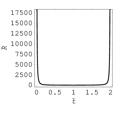
From Figs. 3 and 5, we see that before a crossing of the phantom divide, $F(\tilde{R})$ decreases in terms of $\tilde{R}$ , while that after the crossing, $F(\tilde{R})$ increases in terms of $\tilde{R}$ . The latter behavior is reasonable because in the Hu-Sawicki model [40] of $F(R)$ gravity, which passes the solar system tests, $F(R)$ increases around the present curvature. For $\alpha=2.0$ , the time when a crossings of the phantom divide is the present time, and it follows from Eqs. (19) and (21) that the present value of $\tilde{R}$ is $\tilde{R}_{0}=16.0$ . We remark that such behavior is typical for a general class of viable $F(R)$ gravities introduced in Ref. [41] to which the Hu-Sawicki model belongs. This class of modified gravities can satisfy the solar system tests and unify inflation with the late-time cosmic acceleration. As viable models of $F(R)$ gravity, e.g., the models in Refs. [41, 42, 43, 44, 45, 46, 47] are also proposed. In addition, investigations to solve the problem of a curvature singularity in $F(R)$ gravity [17, 46, 48, 49, 50, 51, 52] have recently been executed in Refs. [53, 54, 55, 56, 57, 58, 59]. Theories without a singularity were also constructed in Ref. [17].

Finally, we mention the stability for the obtained solutions of the phantom crossing under a quantum correction coming from the conformal anomaly. In Ref. [26], it has been shown that the quantum correction of massless conformally-invariant fields could be small when a crossings of the phantom divide occurs and therefore the solutions of the phantom crossing could be stable under the quantum correction, although the quantum correction becomes important near the Big Rip singularity.

IV Conclusion

In the present paper, we have investigated a model of $F(R)$ gravity in which a crossing of the phantom divide can be realized. In particular, we have illustrated the behavior of $F(R)$ gravity around a crossing of the phantom divide by taking into account the presence of cold dark matter. The demonstration in this work can be interpreted as a meaningful step to consider a more realistic model of $F(R)$ gravity, which could correctly describe the expansion history of the universe.

Acknowledgments

The author thanks Professor Chao-Qiang Geng, Professor Shin’ichi Nojiri and Professor S. D. Odintsov for their collaboration in Ref. [26] and important comments very much. He is also grateful to Professor Hideo Kodama for very helpful discussion of related problems. In addition, he acknowledges the KEK theory exchange program for physicists in Taiwan and the very kind hospitality of KEK. This work is supported in part by the National Science Council of R.O.C. under: Grant #s: NSC-95-2112-M-007-059-MY3 and National Tsing Hua University under Grant #: 97N2309F1 (NTHU).

References

[1] Spergel DN et al. [WMAP Collaboration]. First Year Wilkinson Microwave Anisotropy Probe (WMAP) Observations: Determination of Cosmological Parameters. Astrophys. J. Suppl. 2003; 148: 175-194. Peiris HV et al. [WMAP Collaboration]. First year Wilkinson Microwave Anisotropy Probe (WMAP) observations: Implications for inflation. Astrophys. J. Suppl. 2003; 148: 213-231. Spergel DN et al. [WMAP Collaboration]. Wilkinson Microwave Anisotropy Probe (WMAP) three year results: Implications for cosmology. Astrophys. J. Suppl. 2007; 170: 377-408. Komatsu E et al. [WMAP Collaboration]. Five-Year Wilkinson Microwave Anisotropy Probe (WMAP) Observations: Cosmological Interpretation. Astrophys. J. Suppl. 2009; 180: 330-376.
[2] Perlmutter S et al. [SNCP Collaboration]. Measurements of Omega and Lambda from 42 High-Redshift Supernovae. Astrophys. J. 1999; 517: 565-586. Riess AG et al. [SNST Collaboration]. Observational Evidence from Supernovae for an Accelerating Universe and a Cosmological Constant. Astron. J. 1998; 116: 1009-1038. Astier P et al. [SNLS Collaboration]. The Supernova Legacy Survey: measurement of $\Omega_{\mathsf{M}}$ , $\Omega_{\mathsf{\Lambda}}$ and $w$ from the first year data set. Astron. Astrophys. 2006; 447: 31-48. Riess AG et al.. New Hubble Space Telescope Discoveries of Type Ia Supernovae at $z>1$ : Narrowing Constraints on the Early Behavior of Dark Energy. Astrophys. J. 2007; 659: 98-121.
[3] Peebles PJE, Ratra B. The cosmological constant and dark energy. Rev. Mod. Phys. 2003; 75: 559-606. Sahni V. Dark energy: Proceedings of the 11th Brazilian School of Cosmology and Gravitation; July 2004; Rio de Janeiro, Brazil; AIP Conf. Proc. 2005; 782: 166-187 [J. Phys. Conf. Ser. 2006; 31: 115-122]. Padmanabhan T. Cosmological constant: The weight of the vacuum. Phys. Rept. 2003; 380: 235-320.
[4] Copeland EJ, Sami M, Tsujikawa S. Dynamics of dark energy. Int. J. Mod. Phys. 2006; D15: 1753-1935.
[5] Durrer R, Maartens R. Dark Energy and Dark Gravity. Gen. Rel. Grav. 2008; 40: 301-328. Durrer R, Maartens R. Dark Energy and Modified Gravity. arXiv:0811.4132 [astro-ph].
[6] Nojiri S, Odintsov SD. Introduction to modified gravity and gravitational alternative for dark energy. eConf 2006; C0602061:06 [Int. J. Geom. Meth. Mod. Phys. 2007; 4: 115-145], arXiv:hep-th/0601213.
[7] Nojiri S, Odintsov SD. Can F(R)-gravity be a viable model: the universal unification scenario for inflation, dark energy and dark matter. arXiv:0801.4843 [astro-ph]. Nojiri S, Odintsov SD. Dark energy, inflation and dark matter from modified F(R) gravity. arXiv:0807.0685 [hep-th]. Lobo FSN. The dark side of gravity: Modified theories of gravity. arXiv:0807.1640 [gr-qc].
[8] Sotiriou TP, Faraoni V. f(R) Theories Of Gravity. arXiv:0805.1726 [gr-qc].
[9] Caldwell RR, Kamionkowski M. The Physics of Cosmic Acceleration. arXiv:0903.0866 [astro-ph.CO].
[10] Silvestri A, Trodden M. Approaches to Understanding Cosmic Acceleration. arXiv:0904.0024 [astro-ph.CO].
[11] Sami M. A primer on problems and prospects of dark energy. arXiv:0904.3445 [hep-th].
[12] Chakrabarti SK, Saridakis EN, Sen AA. A new approach to modified-gravity models. arXiv:0908.0293 [astro-ph.CO].
[13] Alam U, Sahni V, Starobinsky AA. The case for dynamical dark energy revisited. JCAP 2004; 0406: 008. Alam U, Sahni V, Starobinsky AA. Exploring the Properties of Dark Energy Using Type Ia Supernovae and Other Datasets. JCAP 2007; 0702: 011. Nesseris S, Perivolaropoulos L. Crossing the Phantom Divide: Theoretical Implications and Observational Status. JCAP 2007; 0701: 018. Wu PU, Yu HW. Constraints on a variable dark energy model with recent observations. Phys. Lett. 2006; B643: 315-318. Jassal HK, Bagla JS, Padmanabhan T. The vanishing phantom menace. arXiv:astro-ph/0601389.
[14] Caldwell RR. A Phantom Menace?. Phys. Lett. 2002; B545: 23-29. Nojiri S, Odintsov SD. Quantum deSitter cosmology and phantom matter. Phys. Lett. 2003; B562: 147-152.
[15] Cline JM, Jeon S, Moore GD. The phantom menaced: Constraints on low-energy effective ghosts. Phys. Rev. 2004; D70: 043543.
[16] Amendola L, Tsujikawa S. Phantom crossing, equation-of-state singularities, and local gravity constraints in $f(R)$ models. Phys. Lett. 2008; B660: 125-132.
[17] Abdalla MCB, Nojiri S, Odintsov SD. Consistent modified gravity: Dark energy, acceleration and the absence of cosmic doomsday. Class. Quant. Grav. 2005; 22: L35-L42.
[18] Brevik IH. Crossing of the w = -1 barrier in viscous modified gravity. Int. J. Mod. Phys. 2006; D15: 767-775. Brevik IH. Crossing of the w = -1 barrier in two-fluid viscous modified gravity. Gen. Rel. Grav. 2006; 38: 1317-1328.
[19] Elizalde E, Saez-Gomez D. F(R) cosmology in presence of a phantom fluid and its scalar-tensor counterpart:towards a unified precision model of the universe evolution. arXiv:0903.2732 [hep-th].
[20] Sadeghi J, Setare MR, Banijamali A. String Inspired Quintom Model with Non-minimally Coupled Modified Gravity. Phys. Lett. 2009; B678: 164-167.
[21] Linder EV. Exponential Gravity. arXiv:0905.2962 [astro-ph.CO].
[22] Setare MR. New Agegraphic Dark Energy in $f(R)$ Gravity. arXiv:0908.0196 [gr-qc].
[23] Nojiri S, Odintsov SD. Modified gravity with negative and positive powers of the curvature: Unification of the inflation and of the cosmic acceleration. Phys. Rev. 2003; D68: 123512. Chiba T. 1/R gravity and scalar-tensor gravity. Phys. Lett. 2003; B575: 1-3. Carroll SM, Duvvuri V, Trodden M, Turner MS. Is cosmic speed-up due to new gravitational physics?. Phys. Rev. 2004; D70: 043528.
[24] Perivolaropoulos L. Crossing the phantom divide barrier with scalar tensor theories. JCAP 2005; 0510: 001. Gannouji R, Polarski D, Ranquet A, Starobinsky AA. Scalar-tensor models of normal and phantom dark energy. JCAP 2006; 0609: 016. Nozari K, Sadatian SD. Late-time acceleration and Phantom Divide Line Crossing with Non-minimal Coupling and Lorentz Invariance Violation. Eur. Phys. J. 2008; C58: 499-510.
[25] Yin S, Wang B, Abdalla E, Lin CY. The transition of equation of state of effective dark energy in the DGP model with bulk contents. Phys. Rev. 2007; D76: 124026. Sheykhi A, Wang B, Riazi N. String inspired explanation for the super-acceleration of our universe. Phys. Rev. 2007; D75: 123513.
[26] Bamba K, Geng CQ, Nojiri S, Odintsov SD. Crossing of the phantom divide in modified gravity. Phys. Rev. 2009; D79: 083014. Bamba K. Finite-time future singularities in modified gravity. arXiv:0904.2655 [gr-qc].
[27] Bamba K, Geng CQ. Thermodynamics in $F(R)$ gravity with phantom crossing. Phys. Lett. 2009; B679: 282-287.
[28] Bamba K, Geng CQ. Oscillating phantom in $F(R)$ gravity. arXiv:0909.1249 [astro-ph.CO]. Accepted for publication in Prog. Theor. Phys..
[29] Feng B, Li M, Piao YS, Zhang X. Oscillating Quintom and the Recurrent Universe. Phys. Lett. 2006; B634: 101-105.
[30] Zhang XF, Li H, Piao YS, Zhang XM. Two-field models of dark energy with equation of state across -1. Mod. Phys. Lett. 2006; A21: 231-241.
[31] Feng B, Wang XL, Zhang XM. Dark Energy Constraints from the Cosmic Age and Supernova. Phys. Lett. 2005; B607: 35-41. Li Mz, Feng B, Zhang Xm. A single scalar field model of dark energy with equation of state crossing -1. JCAP 2005; 0512: 002. Zhao GB, Xia JQ, Li M, Feng B, Zhang X. Perturbations of the Quintom Models of Dark Energy and the Effects on Observations. Phys. Rev. 2005; D72: 123515.
[32] Cai YF, Saridakis EN, Setare MR, Xia JQ. Quintom Cosmology: theoretical implications and observations. arXiv:0909.2776 [hep-th].
[33] Nojiri S, Odintsov SD. Modified f(R) gravity consistent with realistic cosmology: From matter dominated epoch to dark energy universe. Phys. Rev. 2006; D74: 086005. Nojiri S, Odintsov SD. Modified gravity and its reconstruction from the universe expansion history: Proceedings of the 29th Spanish Relativity Meeting (ERE 2006): Einstein’s Legacy: From the Theoretical Paradise to Astrophysical Observation; September 2006; Palma de Mallorca, Spain; J. Phys. Conf. Ser. 2007; 66: 012005, arXiv:hep-th/0611071. Nojiri S, Odintsov SD. Modified gravity as an alternative for Lambda-CDM cosmology. J. Phys. 2007; A40: 6725-6732.
[34] Nojiri S, Odintsov SD, Tsujikawa S. Properties of singularities in (phantom) dark energy universe. Phys. Rev. 2005; D71: 063004.
[35] McInnes B. The dS/CFT correspondence and the big smash. JHEP 2002; 0208: 029. Caldwell RR, Kamionkowski M, Weinberg NN. Phantom Energy and Cosmic Doomsday. Phys. Rev. Lett. 2003; 91: 071301.
[36] Barrow JD. Graduated inflationary universes. Phys. Lett. 1990; B235: 40-43. Shtanov Y, Sahni V. Unusual cosmological singularities in braneworld models. Class. Quant. Grav. 2002; 19: L101-L107. Barrow JD. Sudden future singularities. Class. Quant. Grav. 2004; 21: L79-L82. Nojiri S, Odintsov SD. Quantum escape of sudden future singularity. Phys. Lett. 2004; B595: 1-8. Nojiri S, Odintsov SD. The final state and thermodynamics of dark energy universe. Phys. Rev. 2004; D70: 103522. Cotsakis S, Klaoudatou I. Future singularities of isotropic cosmologies. J. Geom. Phys. 2005; 55: 306-315. Barrow JD, Tsagas CG. New isotropic and anisotropic sudden singularities. Class. Quant. Grav. 2005; 22: 1563-1571. Dabrowski MP. Inhomogenized sudden future singularities. Phys. Rev. 2005; D71: 103505. Dabrowski MP. Statefinders, higher-order energy conditions and sudden future singularities. Phys. Lett. 2005; B625: 184-188. Cattoen C, Visser M. Necessary and sufficient conditions for big bangs, bounces, crunches, rips, sudden singularities, and extremality events. Class. Quant. Grav. 2005; 22: 4913-4930. Fernandez-Jambrina L, Lazkoz R. Geodesic behaviour of sudden future singularities. Phys. Rev. 2004; D70: 121503. Fernandez-Jambrina L, Lazkoz R. Classification of cosmological milestones. Phys. Rev. 2006; D74: 064030. Tretyakov P, Toporensky A, Shtanov Y, Sahni V. Quantum effects, soft singularities and the fate of the universe in a braneworld cosmology. Class. Quant. Grav. 2006; 23: 3259-3274. Bouhmadi-Lopez M, Gonzalez-Diaz PF, Martin-Moruno P. Worse than a big rip?. Phys. Lett. 2008; B659: 1-5. Brevik I, Gorbunova O. Viscous Dark Cosmology with Account of Quantum Effects. Eur. Phys. J. 2008; C56: 425-428.
[37] Kolb, Edward W, Turner, Michael S. The Early Universe. Redwood City, California: Addison-Wesley 1990.
[38] Freedman WL et al. [HST Collaboration]. Final results from the Hubble Space Telescope key project to measure the Hubble constant. Astrophys. J. 2001; 553: 47-72.
[39] Riess AG et al.. A Redetermination of the Hubble Constant with the Hubble Space Telescope from a Differential Distance Ladder. Astrophys. J. 2009; 699: 539-563.
[40] Hu W, Sawicki I. Models of f(R) cosmic acceleration that evade solar system tests. Phys. Rev. 2007; D76: 064004.
[41] Cognola G, Elizalde E, Nojiri S, Odintsov SD, Sebastiani L, Zerbini S. A class of viable modified $f(R)$ gravities describing inflation and the onset of accelerated expansion. Phys. Rev. 2008; D77: 046009. Nojiri S, Odintsov SD. Unifying inflation with LambdaCDM epoch in modified f(R) gravity consistent with Solar System tests. Phys. Lett. 2007; B657: 238-245. Nojiri S, Odintsov SD. Modified $f(R)$ gravity unifying $R^{m}$ inflation with the LambdaCDM epoch. Phys. Rev. 2008; D77: 026007.
[42] Starobinsky AA. Disappearing cosmological constant in f(R) gravity. JETP Lett. 2007; 86: 157-163.
[43] Appleby SA, Battye RA. Do consistent $F(R)$ models mimic General Relativity plus $\Lambda$ ?. Phys. Lett. 2007; B654: 7-12.
[44] Amendola L, Gannouji R, Polarski D, Tsujikawa S. Conditions for the cosmological viability of f(R) dark energy models. Phys. Rev. 2007; D75: 083504.
[45] Li B, Barrow JD. Cosmology of f(R) gravity in the metric variational approach. Phys. Rev. 2007; D75: 084010.
[46] Tsujikawa S. Observational signatures of f(R) dark energy models that satisfy cosmological and local gravity constraints. Phys. Rev. 2008; D77: 023507.
[47] Capozziello S, Tsujikawa S. Solar system and equivalence principle constraints on $f(R)$ gravity by chameleon approach. Phys. Rev. 2008; D77: 107501.
[48] Briscese F, Elizalde E, Nojiri S, Odintsov SD. Phantom scalar dark energy as modified gravity: Understanding the origin of the big rip singularity. Phys. Lett. 2007; B646: 105-111.
[49] Appleby SA, Battye RA. Aspects of cosmological expansion in F(R) gravity models. JCAP 2008; 0805: 019.
[50] Frolov AV. Singularity Problem with f(R) Models for Dark Energy. Phys. Rev. Lett. 2008; 101: 061103.
[51] Bamba K, Nojiri S, Odintsov SD. The future of the universe in modified gravitational theories: approaching a finite-time future singularity. JCAP 2008; 0810: 045.
[52] Kobayashi T, Maeda Ki. Relativistic stars in f(R) gravity, and absence thereof. Phys. Rev. 2008; D78: 064019.
[53] Nojiri S, Odintsov SD. The future evolution and finite-time singularities in $F(R)$ -gravity unifying the inflation and cosmic acceleration. Phys. Rev. 2008; D78: 046006.
[54] Dev A, Jain D, Jhingan S, Nojiri S, Sami M, Thongkool I. Delicate f(R) gravity models with disappearing cosmological constant and observational constraints on the model parameters. Phys. Rev. 2008; D78: 083515.
[55] Kobayashi T, Maeda Ki. Can higher curvature corrections cure the singularity problem in f(R) gravity?. Phys. Rev. 2009; D79: 024009.
[56] Capozziello S, De Laurentis M, Nojiri S, Odintsov SD. Classifying and avoiding singularities in the alternative gravity dark energy models. Phys. Rev. 2009; D79: 124007.
[57] Babichev E, Langlois D. Relativistic stars in f(R) gravity. arXiv:0904.1382 [gr-qc].
[58] Upadhye A, Hu W. The existence of relativistic stars in f(R) gravity. arXiv:0905.4055 [astro-ph.CO].
[59] Thongkool I, Sami M, Gannouji R, Jhingan S. The generosity of $f(R)$ gravity models with disappearing cosmological constant. arXiv:0906.2460 [hep-th].

Behavior of F⁡(R)F(R) gravity around a crossing of the phantom divide