The number of cycles of specified normalized length in permutations

The distribution of the number of $k$-cycles in a permutation of $[n]$, for a fixed $k$, converges to a Poisson distribution with mean $1/k$ as $k\to\infty$. In particular the mean number of $k$-cycles and the variance of the number of $k$-cycles are both $1/k$ whenever $n\geq k$ and $n\geq 2k$ respectively. If instead of holding $k$ constant we let it vary with $n$, the number of $\alpha n$-cycles in permutations of $[n]$ approaches zero as $n\to\infty$ with $\alpha$ fixed. So to investigate the number of cycles of long lengths, we must rescale and look at many cycle lengths at once. In particular, we consider the number of cycles with length in some interval $[\gamma n,\delta n]$ as $n\to\infty$. The expectation of the number of cycles with length in this interval is $\sum_{k=\gamma n}^{\delta n}1/k$, which approaches the constant $\log\delta/\gamma$ as $n$ grows large. By analogy with the fixed-$k$ case we might expect the number of cycles with length in this interval to be Poisson-distributed. But this cannot be the case, because there is room for at most $1/\gamma$ cycles of length at least $\gamma n$, and the Poisson distribution can take arbitrarily large values. In the case where $1/\gamma$ and $1/\delta$ lie in the same interval $[1/(k+1),1/k]$ for some integer $k$, the limit distribution has the same first $k$ moments as Poisson($\log\delta/\gamma$). For general $\gamma$ and $\delta$ the situation is considerably more complex but a limit distribution still exists.

In this paper, a “random permutation of $[n]$” will always mean a permutation chosen uniformly at random, and all expectations, distributions, etc. are relative to this choice of probability measure on $S_{n}$, the set of permutations of $n$. The moments of the distributions of the number of $k$-cycles will be very useful, as we will initially express the limit distributions in terms of their moments. We will need both individual and joint moments for the number of $k$-cycles, which we collect here. Let $X_{k}^{(n)}$ denote the number of $k$-cycles in a random permutation of $[n]$. Recall that $(z)_{k}=z(z-1)\ldots(z-k+1)$ denotes the “$k$th falling power” or “$k$th factorial power” of $z$. This notation can be applied to random variables as well.

In particular, we have the following corollary:

Note that Proposition 1 can be expressed in the following way, in light of Corollary 2: the joint factorial moments of numbers of $k$-cycles in random permutations are those of independent Poisson random variables with the same mean unless there is not enough room for the indicated cycles, in which case they are exactly zero. Formulas for the joint power moments of the $X_{k}$ can be derived by expressing them as linear combinations of joint factorial moments.

Our major tool is the following theorem, which expresses the $r$th factorial moment of the number of cycles of a random permutation of $[n]$ with length in $[\gamma n,\delta n]$ as a certain $r$-fold integral.

We can compare this to a number-theoretic result: the expected number of prime factors of a random integer in $[1,N]$ which are at least $N^{\alpha}$, for $\alpha>1/2$, also approaches $-\log\alpha$ as $N\to\infty$. This is but one example of an analogy between prime factorizations of random integers and cycle structure of permutations, developed by Granville in [Gra09+]. This is the simplest example of our general method. We know that the distribution of $X$ is concentrated on two values; thus knowing $\mathbb{E}(X^{(n)})_{0}$ and $\mathbb{E}(X^{(n)})_{1}$ suffices to give the distribution of $X$. In general, if we know that $X$ is concentrated on $k$ values, finding $\mathbb{E}(X^{(n)})_{0},\mathbb{E}(X^{(n)})_{1},\ldots,\mathbb{E}(X^{(n)})_{k-1}$ gives a system of $k$ linear equations in $k$ unknowns which can be solved to determine the distribution of $X$. In order to make stating results easier, we make the following definition.

The $k$th factorial moment of a Poisson($\lambda$) random variable is $\lambda^{k}$. So in a sense, the quasi-Poisson random variables are trying to be Poisson, subject to an upper limit on their value. Let $\pi_{i}(r,\lambda)$ be the probability that a quasi-Poisson($r,\lambda$) random variable has value $i$. Our knowledge of the moments allows us to set up a system of equations to find $\pi_{i}(r,\lambda)$. The solution is given in the following theorem.

We begin by recalling the following lemma.

For a proof, see [Sta99, p. 66-67].

The sum (3) giving $\pi_{i}(r,\lambda)$ consists of the first $r-i$ nonzero terms of the Maclaurin series for $(z^{i}/i!)e^{-z}$, evaluated at $z=\lambda$. Thus if $r$ is large, then $\pi_{i}(r,\lambda)$ approximates the corresponding probability for Poisson random variables.

While the theorems given here only invoke quasi-Poisson distributions of mean at most $\log 2$, in fact we have

The quasi-Poisson($r,1$) distribution is well-known under another name in the study of permutations. It is the distribution of the number of fixed points of a permutation of $[r]$.

We will generally prove convergence of a sequence of random variables to a quasi-Poisson by proving that the factorial moments of that sequence are converging to the factorial moments of a quasi-Poisson. It is known that the moments of a distribution with finite support uniquely determine the distribution [FS09, p. 778]. It is also the case that if $F_{n}(x)$ for $n=0,1,2,\ldots$ are the distribution functions of random variables and

and $F$ is characterized by its moments, then the $F_{n}$ converge in distribution to $F$ [Bil95, Thm. 30.2]. Therefore to show that a sequence of random variables converge to a quasi-Poisson, it suffices to show that the moments converge to those of the quasi-Poisson. The proof of the following theorem is an example.

For example, in a random permutation of $[n]$, for $n$ large, how many cycles have length between $n/4$ and $n/3$? We know that the limiting distribution is quasi-Poisson($3,\lambda$) with $\lambda=\log 4/3$; the values can be found explicitly, and are

One shortcoming of Theorem 9 (and, implicitly, Theorem 4), which the reader may have noted, is that we require $\gamma$ and $\delta$ to be in the same interval of the form $[{1\over k+1},{1\over k}]$ for some integer $k$. This is not accidental; the expressions for the limiting probabilities become much more complicated if this is not the case. However, such expressions still exist.

The integrals of Theorem 3, when ${1\over k+1}\leq\gamma<\delta\leq{1\over k}$, are integrals over $r$-cubes and thus factor easily. In more general circumstances, Theorem 3 gives an integral over some sliced cube, that is, that part of $[\gamma,\delta]^{r}$ in which the sum of the coordinates is less than some constant. Under these circumstances such a factorization is not possible.

Let $1/3\leq\gamma\leq 1/2\leq\delta\leq 1$. By Theorem 3, the probability that a permutation has $i$ cycles of length between $\gamma n$ and $\delta n$, for $i=0,1,2$, approaches a limit as $n\to\infty$. We let these limits be denoted by $p_{i}(\gamma,\delta)$ and obtain explicit expressions for $p_{0},p_{1},p_{2}$.

Let $X^{(n)}$ be the number of cycles of a random permutation of $[n]$ with length in $[\gamma n,\delta n]$. Let $q_{i}(\gamma,\delta)$ denote $\lim_{n\to\infty}\mathbb{E}(X^{(n)})_{i}$ for $i=0,1,2$. We note that

which can be solved for the $p_{i}$ to give

Clearly $q_{0}(\gamma,\delta)=1$ for all $\gamma,\delta$. From Theorem 3 we have

Finally, we have

We must separate into two cases based on the relationship of $\gamma+\delta$ to $1$. If $\gamma+\delta\geq 1$, then the region of integration is a triangle. We have the iterated integral

where $Li_{2}$ is the dilogarithm,

If $\gamma+\delta\geq 1$, then we can just substitute $\gamma$ for $r$ in this integral to get $q_{2}$. (Note that $q_{2}$ does not depend on $\delta$ in this case.) If $\gamma+\delta<1$, then we can break the region of integration into the three rectangles $R_{1}=[\gamma,1-\delta]^{2},R_{2}=[\gamma,1-\delta]\times[1-\delta,\delta],R_{3}=[1-\delta,\delta]\times[\gamma,1-\delta]$ and the triangle $T=\{x,y>1-\delta,x+y<1\}$, as illustrated in Figure 1.

The integrals over rectangles are straightforward; we have already considered the integral over a triangle in (8). Putting everything together, we get

if $\gamma+\delta<1$, and

if $\gamma+\delta\geq 1$.

Finally, from these formulas for the $q_{i}$ we can obtain formulas for the $p_{i}$ using (7).

We now specialize to the case $\delta=1$. Fix some notation: let $Q_{k}(\gamma)=q_{k}(\gamma,1)$ and let $P_{k}(\gamma)=p_{k}(\gamma,1)$. Then we get the formulas

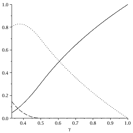
from which we can derive formulas for the $P_{i}(\gamma)$. These formulas give the limiting probability of having $0,1$ or $2$ cycles longer than length $\gamma n$ in a permutation of length $n$, for $\gamma\in[1/3,1/2]$; these probabilities are analytic functions of $\gamma$ in that interval.

In particular, we consider

which applies over $\gamma=[1/3,1/2]$. We have $P_{1}(\gamma)=-\log(\gamma)$ for $1/2\leq\gamma\leq 1$; the probabilities $P_{i}(\gamma)$ for $i=0,1,2$ are shown in Figure 2. Differentiating with respect to $\gamma$ gives

where we have used the fact ${d\over dz}Li_{2}(z)=\log(z)/(1-z)$, which follows from the integral definition (9). Solving for $P_{1}^{\prime}(\gamma)=0$ gives $\gamma_{0}=(1+e^{1/2})^{-1}=0.3775\ldots$. This is the value of $\gamma$ that maximizes the probability of having exactly one cycle of normalized length longer than $\gamma$. We note that it is close to the value of $e^{-1}=0.3678\ldots$ that might be naively expected, since the expected number of cycles longer than $n/e$ is $-\log 1/e=1$. We have $P_{1}(\gamma_{0})=0.8285\ldots,P_{0}(\gamma_{0})=0.0987\ldots,P_{2}(\gamma_{0})=0.0728\ldots$; thus most permutations of $[n]$ have exactly one cycle longer than $\gamma_{0}n$. One might expect the limiting distribution of the number of cycles longer than $n/e$ (or $\gamma_{0}n$) to be Poisson, or at least quasi-Poisson, but the distribution of the number of long cycles is much more strongly peaked. This is because not only is it impossible to have three or more such long cycles, but it is difficult to fit even two; thus to achieve a mean near 1, the value 1 must actually occur quite often.

Finally, we consider some analytic properties of the functions $Q_{k}$.

Note that this recovers the previous formulas (10) for $Q_{1}$ and $Q_{2}$.

It would be interesting to derive, from the recurrence formula in Proposition 12 or otherwise, more numerical results about the $Q_{i}$ or $P_{i}$ – for example, for which $\gamma$ is $P_{2}(\gamma)$ maximized? (Related number-theoretic functions, such as the Buchstab and Dickman functions, can be computed, but clever numerical tricks are necessary; see [Wol03, Ch. 5] and the references therein.)

Granville, inspired by results in number theory, has shown [Gra06, Theorem 5] that the proportion of permutations of $[n]$ with all cycles having length at least $\alpha n$ is given by

where $\omega$ is the Buchstab function, given by

Proposition 12 is reminiscent of this result, and of similar results on the prime factorizations of integers. However, classical number-theoretic results in this vein have focused on the numbers of integers near $n$ with all factors in some fixed normalized interval $[n^{\gamma},n^{\delta}]$. The case $\gamma=0$ (that is, integers with all factors less than $n^{\delta}$) was considered by Dickman [Dic30], and that of $\delta=1$ (all factors greater than $n^{\gamma}$) by Buchstab [Buc49]; the general case was treated by Friedlander [Fri76]. Wolczuk’s thesis [Wol03] compiles many results on the Buchstab function. There do not seem to be results considering the probability that an integer near $n$ has a specified number of prime factors in $[n^{\gamma},n^{\delta}]$, which would be the number-theoretic analogue of the results given here. Similarly, results on the sizes of components of combinatorial structures have in general focused on the lengths of the longest or shortest components. Shepp and Lloyd looked at the longest cycles of permutations [SL66]; more recent work of Panario and Richmond [PR01a, PR01b] has extended this to smallest and largest components of more general decomposable structures.

References

- [ABT03] Richard Arratia, A. D. Barbour, and Simon Tavaré. Logarithmic combinatorial structures: a probabilistic approach. European Mathematical Society, 2003.
- [Buc49] A. A. Buchstab. On those numbers in an arithmetic progression all prime factors of which are small in order of magnitude. Doklady Akad. Nauk. SSSR 67 (1949) 5-8.
- [Bil95] Patrick Billingsley. Probability and measure, 3rd edition. Wiley, 1995.
- [Dic30] K. Dickman, On the frequency of numbers containing prime factors of a certain relative magnitude, Arkiv för Matematik, Astronomi och Fysik 22A:10 (1930) 1-14.
- [Ew72] Warren Ewens. The sampling theory of selectively neutral alleles. Theoret. Population Biol. 3 (1972), 87-112.
- [Fri76] John B. Friedlander. Integers free from large and small primes. Proc. London Math Soc. 3 (1976) 565-576.
- [FS09] Philippe Flajolet and Robert Sedgewick. Analytic combinatorics. Cambridge University Press, 2009.
- [Gra06] Andrew Granville. Cycle lengths in a permutation are typically Poisson. Electronic Journal of Combinatorics 13 (2006), R107.
- [Gra09+] Andrew Granville. Anatomy of integers and permutations. Preprint. Available online at http://www.dms.umontreal.ca/ andrew/preprints.html .
- [Lug09] Michael Lugo. Profiles of permutations. Electronic Journal of Combinatorics 16 (2009), R99.
- [PR01a] Daniel Panario and Bruce Richmond. Exact largest and smallest size of components in decomposable structures. Algorithmica 31 (2001) 413-432.
- [PR01b] Daniel Panario and Bruce Richmond. Smallest components in decomposable structures: exp-log class. Algorithmica 29 (2001) 205-226.
- [SL66] L. A. Shepp and S. P. Lloyd. Ordered cycle lengths in a random permutation. Trans. Amer. Math. Soc. 121 (1966) 340-357.
- [Sta99] Richard P. Stanley. Enumerative combinatorics, volume 1. Cambridge University Press, 1999.
- [Wol03] Dan Wolczuk, Intervals with few prime numbers. Master’s thesis, University of Waterloo, 2003. Available online at etd.uwaterloo.ca/etd/dstwolcz2004.ps .