Ronald Poling \graduationdateDecember2008
Study of Radiative Decays of Psi(2S) Mesons
Abstract
We studied the decay with events collected with the CLEO-c detector. No decays were observed in any of the eleven exclusive decay modes studied. The product branching fraction upper limits were determined for all modes. The 90% confidence level upper limit of was obtained.
There are many people to whom I should show my appreciation and gratitude. This dissertation is completed in the CLEO collaboration, where I learned and experienced a lot in experimental high energy physics. I would like to express my appreciations and gratitude to the people who helped me in various ways.
First I would like to thank my thesis adviser, Ron Poling for his support over the years. His patience, insight and advice have provided me guidance through the process of selecting, designing and performing the analysis. His enthusiasm and passion for physics and way of cooperating with others certainly provide me a good model of a successful physicist. It was a great pleasure to work with him and have him as my adviser.
Pete Zweber cooperate with me on the project that involved in this analysis. From him I have learned a lot of background knowledge about this analysis and general analysis strategies. Datao Gong provided a lot of guidance and advice at the beginning of this project. He shared with me his experience of the previous analysis that invoked the motivations of this project. He also provided great technical helps during the early period of this analysis. During the first year I worked at Wilson Lab of Cornell University, my friend and colleague Selina Li helped me to know the hardware system, to get familiar with the collaboration, and to discuss analyses. I would also like to thank all other current and past CLEO colleagues who work or previously worked at the University of Minnesota, Yuichi Kubota, Dan Cronin-Hennessy, Jon Urheim, Alex Smith, Chris Stepaniak, Brian Lang, Alexander Scott, Tim Klein and Justin Hietala for their advices and helps.
I would like to thank all other people in the CLEO collaboration for their helps and discussions in many aspects, such as hardware, software, and analysis.
I would like to thank Larry McLerran, who was my first year graduate adviser, for his support and guidance during the earlier years.
I would like to thank my family members for their love and support through the years. My father, Chongshou Gao, a theoretical particle physicist, was the first person who told me the importance of experiments in physics. His enthusiasm for physics inspired my interests for physics. My mother, Baiqing Xie, a professor in computer science, showed me the importance of hard work and scientific methods. My brother, Kaizhong Gao, a theoretical condense matter physicist, helped me with his experience doing research both during and outside of his graduate studies. During my difficult time, they all show their endless support to me. I would also like to thank my unborn son, who has not been given his name yet, for the pleasures he has brought to me during the last few months of this dissertation.
Last but not least, I would like to specially thank my husband, You Lin, for his love, friendship, patience, and encouragement through my career. I always have wonderful time with him for discussing about all kinds of topics we can think of. As a theoretical condense matter physicist, he shares with me his thoughts about physics, phylosophy and other areas. His love makes everyday of my life bright and brings smile on my face.
To my family.
Chapter \thechapter Introduction
This dissertation is devoted to the study of the radiative decay of charmonium meson created in annihilations at the center of mass energy of . Specifically, we have studied the radiative decay using CLEO-c detector by reconstructing the final states of decays exclusively. To provide the background for the research I start with the fundamental knowledge of particle physics.
Since the start of human history, the composition of the world has always been a subject of intense interest. From thousands of years ago, when the name atom was given, to recent decades, experimental observations and theoretical studies have allowed us to understand the fundamental nature of materials more and more deeply. The latest and the most successful model of the fundamental particles that compose the universe is the Standard Model, which began with the introduction of quarks by Murray Gell-Mann and George Zweig in 1964. The observation of the top quark completed the quark sector of the Standard Model [1, 2] and provided strong support for the model. It is not a complete description, however, as demonstrated by recent observations of new physics beyond the Standard Model, which may greatly expand our knowledge about the universe.
1 The Standard Model
Nowadays it is common knowledge that all materials are composed of atoms and molecules. Atoms are formed from elementary particles: electrons, protons and neutrons. Since the discovery of the first elementary particle, the electron, in 1897 by J. J. Thomson at the Cavendish Laboratory of Cambridge University, hundreds of elementary particles have been found and various theoretical models have been built to explain the properties and interactions of these particles. For over forty years, the Standard Model has been developed as a framework for understanding and studying these elementary particles. Experimental measurements have demonstrated that the Standard Model provides an excellent description and have provided increasingly precise determinations of many unpredicted parameters.
1.1 Quarks and Leptons
Within the Standard Model, the particles with no known substructure are categorized in three types: quarks, leptons and gauge bosons. The quarks and leptons are the building blocks of composite particles, and are fermions with spin . The gauge bosons are the mediators of the fundamental interactions and have whole-integer spin.
Hadrons are composite particles made of quarks. There are six kinds of quarks and they are characterized according to their “flavor”: , , , , , and (up, down, charm, strange, top, and bottom quarks) with charges (in units of the electron charge) of , , , , , and , respectively. The flavor quantum numbers are the third component of isospin of and quarks, the charm of quarks, the strangeness of quarks, the topness of quarks, and the bottomness of quarks.
The properties of the quarks are summarized in Table 1. Quarks have not been found to exist independently and are only found as constituents of composite particles. The explanation of this is that quarks have another quantum number, color, so named because of similarity with color theory of visible light. Because net color is not observed in nature, the quarks are “confined” into the composite particles called hadrons, which are colorless.
| Flavor | |||||||
|---|---|---|---|---|---|---|---|
| - up | 0 | 0 | 0 | 0 | |||
| - down | 0 | 0 | 0 | 0 | |||
| - charm | 0 | 0 | 0 | 0 | |||
| - strange | 0 | 0 | 0 | 0 | |||
| - top | 0 | 0 | 0 | 0 | |||
| - bottom | 0 | 0 | 0 | 0 | |||
There are two kinds of hadrons. Baryons consist of three quarks and are therefore fermions, e.g. a proton and a neutron . Mesons consist of one quark and one antiquark and are therefore bosons, e.g. and . Hadrons are particles that participate in strong interactions directly.
The Standard Model leptons are the electron (), muon () and tau (), each with charge of , and their corresponding chargeless neutrinos (, and ). Some of the properties of the leptons are given in Table 2 Each lepton type (, , ) is associated with a conserved lepton number. Recent evidence of oscillations among neutrino flavors and nonzero neutrino masses provides the first evidence for physics beyond the Standard Model [3, 4, 5, 6].
| Flavor | Mass | Electric Charge |
|---|---|---|
| - electron neutrino | 0 | |
| - electron | ||
| - muon neutrino | 0 | |
| - muon | ||
| - tau neutrino | 0 | |
| - tau | ||
Tables 1 and 2 show the natural grouping of the quarks and leptons in three generations. Why there are three generations is one of the deepest mysteries of particle physics.
For each quark and lepton there is a corresponding antiquark and antilepton, and as described above the quarks come in three colors. The physical properties of the quarks and leptons from different generations are identical except for the masses of the fermions.
1.2 Intermediate Particles and Fundamental Interactions
The Standard Model describes the electromagnetic, weak and strong interactions. It does not incorporate the fourth of the fundamental interactions, gravitation. Each interaction has its corresponding “force carrier”, particles that are called gauge bosons. These mediators are all bosons with spin . Massless photons () are chargeless and associated with the electromagnetic interaction, which has infinite interaction range. Massive ’s and ’s are associated with the weak interaction, which has a very short range. They are self-interacting and the ’s have electric charge of , while ’s are neutral. Eight massless and chargeless gluons () are associated with the strong interaction, which is also short-ranged because the gluons carry color. As gluons have eight different colors, they not only interact with quarks but also interact with themselves.
1.3 Parameters of the Standard Model
A fundamental feature of the weak interaction in the Standard Model is quark mixing. The weak eigenstates of quarks are not the same as their mass eigenstates. The mixing of flavors and generations induced by weak interactions is parameterized by the Cabibbo-Kobayashi-Maskawa (CKM) matrix, , a unitary matrix, operating on quark mass eigenstates, as shown in Equation 1.
| (1) |
The 2008 Nobel Prize in physics was awarded to M. Kobayashi and T. Maskawa for this formulation, “the discovery of the origin of the broken symmetry which predicts the existence of at least three families of quarks in nature”. Without flavor mixing, quarks could only decay within their generation. We would expect the heavier member to decay 100% of the time to its lighter partner (, ) and the lighter one to be stable. Since the CKM matrix is unitary, the nine elements are reducible to four independent parameters. In the standard parameterization of the matrix, three angles (, , ) and one phase () represent the four independent parameters.
In experimental high energy physics, in addition to the properties of particles such as masses, charges and spins, the fundamental parameters of the CKM matrix must also be measured. These parameters are reflected in the decay widths (lifetimes), branching fractions, and other detailed properties of the particles and their decays. Redundant measurements of the CKM parameters are important and necessary as they are a powerful test on the viability of the Standard Model.
Based on various measurements, the current ranges for the magnitude of the CKM matrix elements have been compiled by the Particle Data Group [7] and are given in Equation 2:
| (2) |
The fact that the coupling between different generations of the quarks is small can be seen from the small values of the non-diagonal elements.
1.4 Symmetries and Conservation Laws
If a system or phenomenon remains unchanged under a transformation of one or more physics variables, then the system or the phenomenon is regarded to have symmetry with respect to this transformation. According to Noether’s Theorem [8], any symmetry of a physical system under a transformation that does not explicitly depend on time has a corresponding conservation law. The interactions and decays of particles are governed by conservation laws.
One type of conservation law is called an exact conservation law. The most commonly used conservation laws, conservation of energy, conservation of linear momentum, conservation of angular momentum, and conservation of electric charge are all exact conservation laws. Conservation of energy is associated with symmetry under time translation. Conservation of linear momentum is a mathematical consequence of symmetry under continuous translation in space. Conservation of angular momentum corresponds to the continuous rotational symmetry of space.
Another type of conservation law is an approximate conservation law. Such a law holds only under some particular situations.
1.4.1 Isospin
Isospin symmetry is an important internal symmetry that was introduced early in the development of nuclear and particle physics. The concept of isospin came from the similarity between neutrons and protons. Neutrons and protons have the same spin of and nearly the same mass, but neutrons are chargeless and protons have unit of electric charge. They behave nearly identically under the strong interactions but differently in weak and electromagnetic interactions. By introducing isospin space, the abstract internal space associated with isospin quantum number , neutrons and protons can be regarded as a doublet of the quantum state with . The algebra of isospin is the same as that of angular momentum and isospin is also an additive quantum number. Therefore protons and neutrons have different projections on the third dimension in isospin space, i.e. for the proton and neutron, respectively. Similarly, pions have isospin of , so by following the algebra of angular momenta, they have three possible third components of isospin, and the corresponding pion states are denoted as , , . The third component of isospin is chosen by convention based on the charge of the particle, e.g. the proton has charge and is assigned the positive value of .
Isospin symmetry is an approximate symmetry describing the strong interaction. The conservation of isospin requires that a system remains unchanged in strong interactions, i.e. the isospin and its third component are conserved. Similar to the relationship between the conservation of angular momenta and the rotational symmetry of space, the conservation of isospin comes from the rotational invariance of strong interactions in isospin space. Conservation laws of isospin does not hold in weak interactions.
1.4.2 Parity
Parity () is a discrete (non-continuous) operation and is defined as the inversion of space coordinates:
| (3) |
According to its definition, parity satisfies . Therefore, it has two eigenvalues, . Under , the signs of both position and linear momentum are reversed, but angular momentum, defined as remains unchanged. Thus and have parity of and has parity of . The classical variables, the time, the energy, the angular momentum of a particle, and masses, charges, coupling constants, etc. satisfy . The variables with include the position, the velocity, the linear momentum of a particle, and electric field.
The invariance under the transformation is associated with conservation of the parity quantum number. Parity is conserved in strong and electromagnetic interactions.
Parity is a multiplicative quantum number, i.e. the parity of a multiparticle state is the product of the parities of all component particles. The wave function of a particle is characterized by its intrinsic parity, which is the parity quantum number of the particle. Basic nonrelativistic quantum mechanics demonstrates that if the orbital angular momentum of a system is , then the parity of the system is the product of and the intrinsic parity. The intrinsic parities of particles are defined in accordance with the conservation law, and are assigned based on experiments and by convention. By convention, quarks have positive parity and antiquarks have negative parity. The intrinsic parity of a hadron can be determined by the strong interactions that produces it, or through decays not involving the weak interaction. The intrinsic parity of a neutral particle can be determined from experiments, e.g. . Photons and gluons have and , respectively. The intrinsic parity of a particle composed of a fermion and antifermion pair is and the intrinsic parity of a particle composed of a boson and antiboson pair is .
1.4.3 Charge Conjugation
Another discrete transformation is the charge conjugation () transformation, which turns a particle into its antiparticle. The charge conjugation operator reverses the electric charge and all the internal quantum numbers, including lepton number, baryon number, , strangeness, and the other flavors. The eigenvalue of , , is called charge conjugation parity (), similar to parity. Only truly neutral systems with all quantum charges and magnetic moment zero are eigenstates of charge parity. Photons and gluons both have parity . For a system that is composed of a particle and antiparticle pair, if the orbital angular momentum is and the sum of the spin angular momenta of the two particles is , the parity is . parity is also a multiplicative quantum number.
Invariance under the charge conjugation transformation leads to the conservation of charge parity and is called -symmetry. -symmetry holds in strong and electromagnetic interactions, and even gravitational interactions. However, weak interaction does not obey charge conjugation symmetry.
1.4.4 Other Conservation Laws
There are other conservation laws, e.g. conservation of strangeness and baryon number, that also govern elementary particle interactions. The strangeness , defined as the number of strange antiquarks minus the number of strange quarks , is a quantum number introduced to describe decays of particles in strong, electromagnetic and weak interactions. It has been observed experimentally that the change of the strangeness quantum number satisfies for strong and electromagnetic interactions and for weak interactions.
Baryon number is defined as one third of the difference between the number of quarks and the number of antiquarks , where the fraction one third comes from the fact that a baryon consists of three quarks or antiquarks. The conservation of baryon number holds in all interactions of the Standard Model. Lepton number is similarly conserved in all interactions.
More detailed descriptions and discussions about conservation laws can be found in any standard textbook, such as Ref. [9].
2 Charmonium States
Quarkonium is a flavorless bound state which consists of a quark and its own antiquark bound by strong interactions. Quarkonia include charmonia and bottomonia. A charmonium meson( meson) is the bound state of a charm quark and a charm antiquark, and a bottomonium meson ( meson) is the bound state of a bottom quark and a bottom antiquark. No toponium exists because of the large mass of top quark and antiquark. The quark would decay through electroweak interactions before a bound state can form. Bound states of light quark and antiquark pairs are normally not called quarkonium, partly because in the experiments the states observed are usually the mixture of the light quark states. The large mass difference between the charm or bottom quark and the lighter quarks prevents the charmonium and bottomonium states from mixing with each other or with the lighter flavorless mesons. Charmonium and bottomonium are very important for studying the strong interaction. The two charmonia involved in this dissertation are the (often written as or ) and (often written as ).
The charmonium resonances were first discovered in experiments in 1974 [10, 11, 12], known as the “November Revolution,” when the meson was independently discovered by a group at the Stanford Linear Accelerator Center and by a group at Brookhaven National Laboratory. The charmonium resonances were quickly interpreted as bound states and were very powerful in establishing the reality of quarks and the Standard Model.
Non-perturbative Quantum chromodynamics (QCD) is used to compute the properties of mesons. Similar to nonrelativistic models of the hydrogen atom, the motion of the quarks in a quarkonium state is nonrelativistic so they can be assumed to move in a static potential. One technique that can be effectively applied to quarkonium is application of quantum mechanics, with specific choices of the quark-antiquark potential. Such calculations predict the masses of quarkonia states, and can be directly tested with data. One of the candidate potentials is [13]
| (4) |
where is the effective radius of the quarkonium state and and are parameters. The first term is the Coulomb-type force that dominates at the short distances (asymptotic freedom). It corresponds to the potential induced by one-gluon exchange between the quark and its anti-quark, analogous to the Coulomb electromagnetic potential. The second term is linear in and produces quark confinement.
The charmonium states, as well as other elementary particles, are denoted with the spectroscopic notation . The principal quantum number represents the ground state, and successive excited states of the particle. represents the spin of the particle, which for charmonium takes values , since its quark and antiquark constituent are fermions and have spin projections of or . denotes the orbital angular momentum and the letters , , … stand for … . is the total angular momentum with . Specific states are frequently denoted by their , where and are the parity and charge conjugation quantum numbers, respectively. For example, the two charmonia involved in this dissertation are and . The means that for these states, and . In fact, denotes and is , so has and has . The total angular momenta are for and for . According to the parity convention for quarks and antiquarks, both and have parity . However, the parity of is and that of is because . Thus the characterization of is and that of is .
The charmonium state and are the first excited states of and respectively. Therefore the transition between and is similar to the transition between and . The lowest energy states for mesons with quark-antiquark pairs have and negative parity and are called pseudoscalar mesons, e.g. and . For excited states of mesons the quark spins are parallel, so if a state has zero orbital angular momentum, then the total angular momentum of the particle is . Such states are called vector mesons, e.g. and . As the vector mesons have the same quantum numbers as photons (virtual photons), i.e. , they can be produced directly in collisions, in which virtual photons are formed. Other charmonium states can be observed in the transitions of states or in collisions. Figure 1 shows the spectrum of the charmonium resonances and the observed transitions among them.

3 Production at
3.1 Decays
The charmonium states with have four possible ways to decay, as shown in Figure 2. In experiments, they are observed to be through leptonic decays, hadronic decays, and radiative decays.
- (a)
Leptonic decays (Figure 2(a)): The quark and antiquark pair annihilate to create a virtual photon and then the virtual photon produces a lepton and antilepton pair, i.e. .
- (b)
Hadronic decays by the electromagnetic interaction (Figure 2(b)): The quark and antiquark pair annihilate to create a virtual photon and then the virtual photon produces a quark and antiquark pair. The quark-antiquark pair fragments into a final state of hadrons, i.e. .
- (c)
Hadronic decays by the strong interaction (Figure 2(d)): The quark and antiquark pair annihilate to three gluons, then the three gluons fragment into a final state of hadrons, i.e. .
- (d)
Radiative decays (Figure 2(c)): The quark and antiquark pair annihilate to a photon and two virtual gluons, then the two gluons produce the final state of hadrons, i.e. .


The strong interaction dominates over the electromagnetic interaction, in spite of the suppression (OZI) of the three-gluon process. It is impossible for a charmonium state with to decay to a single gluon as the particle is colorless but a gluon carries color charge. Decay through two gluons is forbidden by conservation. For example, of mesons decay to hadrons through three gluons and only of mesons decays to hadrons through virtual photons.
3.2 Radiative Decay of
The meson has a mass of () MeV and can decay radiatively to another meson, such as and . The radiative decay , that is the focus of this dissertation, has not been observed.
In our investigations, mesons are produced by the annihilation of electron-positron pairs at a center-of-mass energy of . An unknown portion of the mesons would decay into a transition photon and a pseudoscalar meson through electromagnetic interaction. Some of the generated mesons would decay into hadrons, ultimately into detectable particles, like pions, kaons, and photons. The first step of the radiative decay is a two body decay, which means the particle could be observed and measured through the energy distribution of the transition photon.
The experimental challenge of the measurement for this decay channel is to detect the MeV radiative photons in an experimental environment with considerable background. Inclusive study is impractical for these low photon energies. Our alternative approach is to study the decay exclusively by reconstructing from its hadronic decay products and looking at the candidate mass for evidence of .
3.3 Theoretical Background of
The purpose of this analysis is to study the direct magnetic dipole (M1) radiative transition by reconstructing exclusive decays of the . The partial width for a direct M1 radiative transition between S-wave charmonium states is given by
| (5) |
where is the fine structure constant, () is the charge (mass) of the charm quark, and is the energy of the transition photon. The factor incorporates the matrix element for the spin-flip transition of the pair. The energy of the transition photon is determined by the mass difference between the S-wave spin-triplet and spin-singlet charmonium states and therefore is related to the hyperfine mass splitting between them.
The hyperfine mass splitting is defined as
| (6) |
where denotes the principal quantum number, is the strong coupling constant, and is the wave function of the S-wave spin-triplet state at the origin. Table 3 lists the theoretical predictions for the hyperfine splitting. The splitting of the first radially excited state is consistently less than that for the ground state, reflecting coupled-channel effects between the and the nearby open-charm threshold [14, 15, 13].
Table 4 lists the theoretical predictions for the branching fraction. These include phenomenological models, including nonrelativistic potential models, effective field theory calculations, and QCD calculations implemented via lattice gauge theory (LQCD). The results fall in the range . \singlespacing
| Ref. | [MeV] | [MeV] |
|---|---|---|
| Experiment[7] | 484 | 116.51.2 |
| Potential Model[16] | 92 | 119 |
| Potential Model[17] | 83 | 130 |
| Potential Model[18] | 42-65 | 99 |
| Potential Model[19] | 49 | 78 |
| Potential Model[20] | 70 | 113 |
| Potential Model[21] | 72-109 | 121-196 |
| Potential Model[22] | 60 | 130 |
| Perturbative QCD[23] | 69.0 | 101.0 |
| Potential Model[24] | 71 | 116 |
| Potential Model[25] | 204 | 139 |
| Potential Model[26] | 86 | 117 |
| Potential Model[27] | 78 | 117 |
| HQET[28] | 60 | 100 |
| Potential Model[29] | 68.0 | 117.8 |
| Potential Model[30] | 54.2-82.5 | 106.1-128.3 |
| Potential Model[31] | 98 | 117 |
| BSLT[32] | 38 | 102 |
| Quark Model[33] | 98 | 117 |
| Phenomenology[34] | 578 | — |
| Perturbative QCD[35] | 3735 | 8826 |
| Potential Model[14] | 46.1 | 117* |
| Quark Model[36] | 51 | 119 |
| Potential Model[37] | 42-53 | 108-123 |
| Potential Model[38] | 38-41 | 80-108 |
| Potential Model[39] | 66.9-88.4 | 115.22-117.06 |
| Quenched LQCD[40] | 3425 | 72.60.9 |
| Unquenched LQCD[41] | -18189,12424 | 801,10519 |
*Input to theory, not a prediction.
| Ref. | [MeV] | [] |
|---|---|---|
| Experiment[7] | 484 | — |
| Potential Model[13] | 24.9(49.6) | 0.585(4.45) |
| Potential Model[42] | 48* | 3.1 |
| Potential Model[21] | 92 | 0.6-27.0 |
| Potential Model[22] | 60 | 8.0 |
| Potential Model[43] | 92 | 13.4-20.2 |
| Potential Model[44] | 32 | 1.2 |
| Quark Model[33] | 32(91) | 1.3(29) |
| BSLT[45] | 46 | 0.89 |
| Potential Model[37] | 48 | 5.0-6.2 |
| Potential Model[39] | 66.9(88.4) | 12(36) |
| Phenomenology[46] | 47.8 | 2.60.7 |
*Calculated using mass values from Ref. [7].
3.4 Estimates of Production and Decay Rates
The PDG does not provide enough information for the branching fractions of and for definite predictions of event rates in any experiment. We have made certain assumptions to estimate these values for our analysis.
An estimate of expected rate can be based on the similarity between and . We start from the transition rate between spin-0 and spin-1 S-wave states, which is given in Equation 5. For estimate, we assume the matrix element is the same for both decays and use the mass differences to calculate the energies of transition photons. For the decay, we have
| (7) |
where () is the mass of the MeV ( MeV). Similarly, for the decay, we have
| (8) |
From the branching fraction for ,
| (9) |
and the full width of ,
| (10) |
we can obtain the partial width of :
| (11) |
With the above information the partial width of can be calculated as
| (12) | |||||
The full width of is
| (13) |
Therefore, the branching fraction of is estimated to be
| (14) |
To estimate the expected number of produced events for each decay mode considered, we need estimates of the branching fractions of , where is a particular final state. These are estimated by scaling from the corresponding branching fractions:
| (15) | |||||
3.5 Previous Measurements of Productions and Decays
In this analysis we are motivated to measure the mass of the from the decay channel , and improve the measurement of full width of the . Previous measurements compiled by the PDG give an average of on the mass and on the full width of in 2005 [7]. The measurements that contributes to the average of PDG 2006 are from CLEO, and with 61 events in 2004 [47, 48, 49], from BaBar, and with events in 2004 [50], and from Belle, with events in 2002 [51]. In the CLEO measurement, two-photon production of , followed by was studied with samples of CLEO II/II.V data and of CLEO III data. The result was a measurement of the ratio . The most recent average of measurements gives a small correction of the mass of from to , but the width has remained unchanged since 2006 [52]. In the BaBar measurement, the mass and width were measured with a sample of collected at the . In 2006, BaBar inclusively studied the decay with a sample of collected at the , finding , with a significance of [53]. This result is listed in PDG 2008 [52]. In a recent BaBar measurement and , where was studied with a sample of collected at the . They measured the ratio of and to the corresponding process. Using the result from the PDG 2008, this leads to . However, the mass resolutions of the two separate modes and are very different and the peaks of and overlap each other [54]. In a recent Belle measurement, two-photon production of , followed by or , was studied with a sample of collected at the , leading to results of and at 90% confidence level [55].
4 Objectives and Organization of this Dissertation
Information about production and decay is currently very limited. Measurements at the energy are hampered by serious backgrounds and limited to only a few modes. Measurements in the cleaner environment of annihilations near charm threshold have significant advantages. This is the principal motivation for the work described in this dissertation.
Starting in fall 2003, the CESR-c/CLEO-c program began an anticipated three year run though the actually run period was 4.5 years until the shut down on March 2, 2008. During this period, the CLEO-c detector was used to collect the following data:
- •
of integrated luminosity on the (see Section 5.4)
- •
about million decays
- •
of continuum below the
- •
of scan data near
- •
of data at
- •
about of data at for physics
While the data samples were smaller than the original project goals, the CLEO-c project is regarded as a great success.
In this project, the decay channel is investigated through the exclusive reconstruction of candidate events in the CLEO-c data sample. A similar nearby decay channel, , has been studied for validation and comparison purpose, using CLEO’s previous measurement of this channel.
Based on the current information about the decay , we evaluated the project by making an estimate on the number of evens that can possibly produced.
For the CLEO-c sample of 25.9 million events, the estimated number of events produced is , where we have used a branching fraction of . With this information, the expected numbers of produced events of all considered modes are listed in Table 5. The error in is dominated by , and the error in is dominated by .
| Mode | produced | ||
|---|---|---|---|
| (%) | |||
| – | – | – | |
| – | – | – |
The expected number of produced was estimated assuming a full width of MeV for according to PDG average [7]. We expected that the measurement can be improved with a larger CLEO-c sample based on these PDG values as discussed in Chapter Study of Radiative Decays of Psi(2S) Mesons.
From the above estimate we find that the measurement of the decay is possible in spite of technical challenges and the lack of previous knowledge on the physical properties of . If enough events can be observed we also plan to measure the partial width of . The only previous contribution to the measurement was given by CLEO, in 2004, which is [47, 48, 49].
Following this introduction, the remainder of this dissertation is organized as follows. The CESR-c accelerator and CLEO-c detector are described in detail in Chapter Study of Radiative Decays of Psi(2S) Mesons. The analysis set up and the event-selection criteria, as well as the study of the related decay channel are included in Chapter Study of Radiative Decays of Psi(2S) Mesons. In Chapter Study of Radiative Decays of Psi(2S) Mesons the summary, discussions and conclusions of the investigation of the radiative decay are presented.
Chapter \thechapter Experimental Apparatus
The analysis presented in this dissertation was based on data collected with the accelerator and detector at the Cornell University Laboratory of Elementary Particle Physics. The design, construction and operation of the apparatus has been carried out by the collaboration of hundreds of people. In this chapter the Cornell Electron Storage Ring (CESR-c) is described in Section 5 and the CLEO-c detector in Section 6. The trigger and data acquisition systems are described in Section 6.7 and event reconstruction in Section 7. Finally, Section 8 explains the simulation of the detector response for determination of the detection efficiencies and backgrounds for measurements of various physical processes.
5 Cornell Electron Storage Ring - CESR-c
The Cornell Electron Storage Ring running at charm threshold (CESR-c) is a symmetric electron-positron collider with a circumference of 768 meters. It is located at Wilson Synchrotron Laboratory, about forty feet under the track-and-field facility of Cornell University. Accelerators like CESR-c produce short-lived particles under controlled conditions, allowing more detailed studies than with particles from natural sources like cosmic rays. In CESR-c, electrons and positrons annihilate via the electroweak interaction to produce final states consisting of hadrons and leptons. These annihilations occur inside the CLEO-c detector, which measures the particles’ momenta, energies and other properties.
CESR-c is designed to produce collisions between electrons and positrons with center-of-mass energies between 3 and 5 GeV. For the data sample used for this dissertation, the beam energy was set at around 3.7 GeV, to produce charmonium mesons nearly at rest. CESR-c consists of three parts: the linear accelerator (Linac), the CESR synchrotron, and the storage ring, as shown in Figure 3.

5.1 Linac
The Linac is the first part of the CESR-c, in which electrons and positrons are generated, collected, bunched and accelerated before they enter the synchrotron for further acceleration.
The electrons are boiled off of a hot filament by thermionic emission. They are accelerated to 150 keV by static electric fields and injected into the 30-meter-long vacuum pipe which is the main Linac structure. The Linac has eight radio-frequency (RF) cavities, which generate oscillating electric fields that accelerate the electrons to an energy of 300 MeV before they are injected into the synchrotron.
The positrons are created by intercepting the 150 MeV accelerated electrons halfway down the Linac and directing them into a tungsten target. Showers of electrons, positrons and photons are generated from the target. Positrons are selected by a magnetic field and then accelerated along the rest of the Linac to a final energy of 200 MeV for injection into the synchrotron.
5.2 Synchrotron
The synchrotron is a circular vacuum pipe that fills the CESR-c tunnel and consists of four RF accelerating cavities of 3-meter length and 192 bending and focusing magnets. The RF cavities add energy to the electrons and positrons each time they pass through. Dipole magnets bend the trajectories of the electrons and positrons so that they can move along the circular path within the synchrotron. Quadrupole and other focusing magnets keep the electrons and positrons confined to trajectories near the axis of the beam pipe. As the radius of the circular motion of electrons and positrons is given by , in order to keep the particle beam bunches moving in synchrotron, the dipole magnetic field needs to be synchronized with the momentum increase of the particles. It takes about 1500 revolutions or 1/100 second to accelerate the particles to the desired beam energy, after which they are injected into the CESR-c storage ring. At the typical beam energy of 2 GeV , the beam particles travel at 99.999997% of the speed of light.
5.3 CESR-c Storage Ring
Once the electron or positron beam has been accelerated to the desired energy, it is injected into the storage ring which operates by the same principle as the synchrotron. The electrons and positrons travel in a closed orbit in a much better vacuum than the synchrotron. The storage ring contains 106 quadrupole focusing magnets and 86 dipole bending magnets, and in addition it also has sextupole and octupole magnets for very precise focusing of the beams. When the electrons and positrons circulate in the ring, they emit electromagnetic radiation that causes energy loss, which is called synchrotron radiation. The energy is restored by superconducting radio-frequency (RF) cavities that operate at a frequency of 500 MHz. These RF cavities are similar to those used in the Linac and synchrotron, except that they are used primarily to restore the energy of the particles, while those in the Linac and synchrotron are used to accelerate the particles.
The synchrotron radiation deposits energy in the vacuum chamber wall and the generated heat due to the radiation is carried away by circulating water. Some of the synchrotron radiation is used by the Cornell High Energy Synchrotron Source (CHESS) facility for X-ray research in the areas of physics, chemistry, biology, environmental science, and materials science.
In standard operation CESR-c stores the particles in 45 bunches of electrons and 45 bunches of positrons (configured as nine “trains” of five bunches), circulating in opposite directions. They are allowed to cross at one interaction region, where the CLEO-c detector is located. One “fill” of electrons and positrons lasts about one hour. Since both the electron and positron bunches are stored in the same ring, four electrostatic separators are used to set up “pretzel” orbits and ensure that the electrons and positrons miss each other when they pass through the unwanted intersecting locations, sometimes referred to parasitic crossings. Thus the electrons and positrons collide only at the interaction point, which is at the center of CLEO-c detector. Figure 4 shows a greatly exaggerated [56]

schematic of the pretzel orbits. At the interaction point, the two beams are steered into each other and collide at a small crossing angle of approximately mrad ().
5.4 Luminosity
The annihilation rate depends on the “luminosity” of the storage ring, which in turn depends primarily on the stored current and beam size. Instantaneous luminosity is defined as the number of collisions for each cm2 of cross section per second by the approximate equation
| (16) |
where is the frequency of revolution of the particles, is the number of electron or positron bunches in the beam, and are the number of electrons and positrons in each bunch respectively, and is the cross-sectional area of the beams. The total number of events for a particular process, , is given by
| (17) |
where is the cross section for the process. The integral of the instantaneous luminosity, , is generally referred to as the integrated luminosity or luminosity. In CLEO-c, the integrated luminosity for a given data sample is determined by a weighted average of the results from three processes , , and , for which the cross sections are precisely determined by QED. Each of the three final states relies on different components of the detector with different systematic effects [57].
5.5 CESR-c Upgrades
CLEO-c and CESR-c have been developed from the previous CLEO III detector and CESR accelerator. For over 20 years beginning in 1979, CESR collected electron-positron annihilation data at a center-of-mass energy of GeV for the study of mesons near threshold. For the CLEO-c and CESR-c project, CESR was proposed to run around charm threshold, 3-5 GeV. Modifications to the accelerator and detector were necessary to accommodate the lower center-of-mass energy.
As the rate of the synchrotron radiation is proportional to , the reduction of the beam energy greatly altered the beam dynamics. The decrease of the synchrotron radiation affects CESR performance through two important beam parameters: damping time, with which perturbations in beam orbits caused by injection and other transitions decay away, and horizontal beam size, or horizontal emittance, which measures the spread of particles in the bend plane. At decreased center-of-mass energy, these effects can limit the luminosity to unacceptable levels. In CESR-c, superconducting wiggler magnets were used to increase the synchrotron radiation [56], reduce the damping time, and increase the luminosity. A wiggler magnet is a series of dipole magnets with high magnetic fields. Each successive dipole has its direction of magnetic field flipped. When a particle passes the wiggler, it will oscillate and therefore emit additional synchrotron radiation while keeping the overall path of the particle in the ring the same. The damping time is decreased and the horizontal beam size is increased because of increase of the synchrotron radiation. CESR-c included twelve superconducting wiggler magnets for low-energy running.
6 CLEO-c Detector
When an electron and positron collide and annihilate, the flash of energy results in the creation of new matter. The CLEO detector, named for the one historically coupled to Caesar, was built to study these collisions, with details described in References [58, 59].
The CLEO-c detector was the final stage of a series of upgrades of the CLEO detector since its commissioning in 1979. Beginning in 1989, the CLEO II detector was a productive source of physics research, due to its very good drift chamber based tracking system and outstanding electromagnetic calorimeter. In 1995, after a three-layer silicon strip vertex detector and a new beam-pipe were installed, and an argon-ethane gas mixture in the drift chambers was switched to helium-propane, CLEO II was upgraded to CLEO II.V. A few years later CLEO II.V was upgraded to CLEO III by adding a Ring Image Cherenkov (RICH) detector for particle identification and a new tracking system, which consisted of a new central drift chamber surrounding a four-layer silicon strip vertex detector. The conversion from CLEO III to CLEO-c in 2003 consisted of the replacement of the silicon vertex detector with a low-material gaseous tracking detector (ZD).
6.1 CLEO-c Detector
The CLEO-c detector (Figure 5) measures about 6 meters on a side, and is constructed of about 900,000 kilograms of iron and over 25,000 individual detection elements. It is an approximately cylindrically symmetric detector aligned along the beam line, and covering about 93% of the solid angle. Electrons and positrons collide at the interaction point (IP) in the beam pipe, which is located at the center of the detector. The annihilation produces new particles, which decay quickly into long-lived or stable charged particles, electrons, muons, protons, pions, and kaons, and some neutral particles including photons. Particles pass through different sub-detectors of the CLEO-c detector, leaving measurable signals. The tracking system provides the precise measurement of the trajectories of charged particles and information on the rate of energy deposit in the material (). The Ring Imaging Cherenkov (RICH) detector provides a velocity measurement for charged particle identification. The electromagnetic crystal calorimeter (CC) is used to measure the energies of electrons and photons. A superconducting solenoid provides a uniform magnetic field over the whole tracking system, RICH and CC. The muon detector is used to detect muons, which can penetrate all inner sub-detectors if they have sufficient momentum.
The whole operation of the experiment includes the constant calibrations, event data taking process and offline data analysis, which includes the Monte Carlo studies and physics analysis.

6.2 Tracking System
The tracking system of CLEO-c consists of two drift chambers, which provide precisely measured space points for charged particles emerging from the interaction. These devices reside inside a superconducting solenoidal magnet that provides a uniform field of 1 T along the beam direction. The tracking system measures the helical trajectories of charged particles, and online and offline software reconstruct these trajectories to obtain precise measurements of particle momenta.
6.2.1 Inner Drift Chamber - ZD
The innermost sub-detector of the CLEO-c detector is the inner drift chamber (ZD), which is located right outside of the beam pipe. The major hardware modification from CLEO III to CLEO-c is the replacement of the Silicon Vertex Detector with the wire vertex drift chamber ZD. The silicon vertex chamber, as the tracking drift chamber for CLEO III, was used to provide extremely accurate track position measurements in and as close as possible to the interaction point for studies at the . However, when the center of mass energy was reduced from 10 GeV down to 3-5 GeV, the momentum distribution of the charged tracks is shifted down to lower values. Minimizing material is crucial at lower center-of-mass energies since multiple scattering dominates the momentum measurement error for low momentum tracks. As the tracks have lower velocities, the importance of vertexing is reduced because vertex separation for decays of particles like and are too small to be resolved with the silicon vertex detector. Since the extreme precision of the previous silicon vertex detector was not needed and the material was a disadvantage, it was replaced with the ZD chamber [60].

The ZD is located just outside the beam pipe and covers radii from 4.1 cm to 11.8 cm from the interaction point. An isometric view of the structure of the ZD is shown in Figure 6. It supports gold-plated tungsten sense wires and gold-plated aluminum field wires. The sense wires are in six layers with the number of cells per layer ranging from 34 to 66 for a total of 300. Each cell measures mm and consists of a sense wire held at V, surrounded by field wires at ground. Cells share bordering field wires. The wires are oriented at a small (stereo) angle with respect to the beam axis, allowing measurement of , and . The stereo angle of the ZD ranges from in the innermost field wire layer to in the outermost field wire layer, with the stereo hyperbolic sag of 4 mm. The “all stereo” design optimizes the measurement of (position in the beam direction), from which the inner drift chamber was given the name “Z Detector.” The ZD’s stepped structure provides spatial measurement of charged particles within , where is the angle of the the particle with respect to the beam.
When a charged particle passes through a cell, it ionizes the atoms of gas filling. The ZD is filled with a very pure mixture of 60% helium and 40% propane (C3H8) which provides a very long radiation length ( m) [56]. The electrons produced from the ionized atoms are accelerated toward the sense wire and away from the field wires. As the electric field increases toward the sense wire, these primary electrons ionize other gas atoms and create an “avalanche” at the sense wire. The time of the electric pulse observed on the sense wire and the charge, which is related to the deposited energy, are recorded. This information is used to map out the trajectories of the charged particles and to fit tracks.
6.2.2 Main Drift Chamber - DR
Outside of the ZD detector is the main drift chamber (DR), a much larger device that measures particles out to a distance of 0.8 m from the interaction point. The main drift chamber has design similar to that of the ZD, but with much larger size. It has 9,796 gold-plated tungsten sense wires and 29,682 gold-plated aluminum field wires, arranged in 47 layers. The wires are grouped in nearly square cells, with cell size 14 mm. Each cell contains one sense wire surrounded by eight field wires. The voltage on the sense wires is V with respect to the grounded field wires. The gas in the DR is the same as the gas in the ZD, a mixture of 60% helium and 40% propane. Among the 47 layers of wires, the first 16 are axial and the remainder are stereo layers that alternate angles about in groups of four to provide information throughout the volume of the detector. In order to determine the position of the particle at the stereo layer, the axial layers are used to predict the particle’s position and to match the information from the stereo wires. The inner and outer radii of the drift chamber are covered with longitudinally and azimuthally segmented cathodes to provide precise measurements of the position of most tracks as they enter and emerge from the DR.
6.2.3 Hadron Identification by Specific Ionization -
Information about the rate of energy loss is provided by the DR for each charged particle, along with the the measured momentum. This can be used for particle identification. The energy lost per unit length depends upon a particle’s velocity, as given by the Bethe-Bloch formula. A variable is formed for each particle hypothesis of electron, muon, pion, kaon, or proton. The value of is the sum of over a lot of hits. is defined for hit as
| (18) |
where is the uncertainty of the measurement, usually approximately 6%. Figure 7 shows the measured as a function of momentum for a large population of charged particles. At momenta below 500 MeV, pions and kaons are well separated. At higher momenta, the information is limited and additional information is needed for good particle identification.

6.2.4 Track Reconstruction
Track reconstruction is the process to form tracks with hits, the electrical signals from the wires, using a pattern-recognition algorithm on three-dimensional ( and ) position measurement from the ZD and DR. (The resolution varies over the cell and is of order .) Once tracks are found they can be fit to determine interesting physics quantities like momenta, vertex positions and directions [61]. The CLEO-c fitter is an implementation of the Billoir or Kalman algorithm that optimizes the determination of the momentum and trajectory, taking into account the expected energy loss.
The tracking system is within an axial magnetic field of 1 T. The charged particles follow helical paths within the constant magnetic field. As the magnetic field is parallel to the axis, the transverse momentum , in the plane, can be related to the curvature of a particle’s trajectory by
| (19) |
where is the magnitude of the particle’s charge, is the magnitude of the magnetic field, and is the radius of curvature. Therefore, the measurement of the full momentum vector can be obtained by the measurement of the track’s curvature in , and its angular coordinates and . At 1 GeV the momentum resolution of the charged particle is about 0.6%. The direction of the curvature within the magnetic field indicates the sign of the charged particle.
6.3 RICH Detector
The Ring Image Cherenkov Detector (RICH) [62, 63] is located directly outside of the main drift chamber. It was the most significant improvement in the CLEO III upgrade from CLEO II.V and was not modified for CLEO-c. The measurement of Cherenkov radiation in the RICH provides the additional charged particle identification needed for the higher momenta where is inadequate.
When a charged particle passes through a transparent dielectric medium at a speed greater than the speed of light in that medium, electromagnetic radiation, called Cherenkov radiation is produced. This effect was first observed by Cherenkov in 1934. As a charged particle travels through the medium, its electromagnetic field disturbs the local electromagnetic field in the medium, and displaces and polarizes the electrons in the atoms of the medium. Photons are emitted when the electrons of the medium return to their equilibrium state. When the charged particle travels at a speed higher than the speed of light in the medium, the photons constructively interfere to make the radiation observable. The radiation is produced in a cone with its central axis along the trajectory of the traveling particle. The characteristic angle of the cone , known as Cherenkov angle, is related to the velocity of the particle by
| (20) |
where is the index of refraction of the dielectric medium, and is the ratio between the velocity of the charged particle and the speed of light . With the relations and the cosine of the Cherenkov angle can be expressed in terms of index of diffraction , mass of the charged particle , and momentum of the charged particle by
| (21) |
If the momentum of the charged particle can be measured independently, such as by fitting the trajectory in the tracking system, then the Cherenkov angle gives the mass and therefore the identity of the charged particle.
The RICH detector is shown in Figure 8 and covers 83% of the solid angle. The innermost parts of the RICH

detector are the radiators, which are made from LiF and have an average thickness of 1.7 cm. For CLEO-c’s magnetic field of 1 T, tracks with transverse momenta of 0.12 GeV/ reach the RICH radiators. When a charged track passes through the radiators, Cherenkov photons are produced. There are a total of 14 rows of radiators and the four central rows contain “sawtooth” radiators, with triangular grooves on the surface, to overcome the total internal reflection for Cherenkov photons produced with nearly normal track incidence. The outer rows of radiators are flat. The Cherenkov photons produced in the radiators propagate outward through an expansion volume filled with pure nitrogen, which is transparent to Cherenkov photons with the characteristic wavelength of about 150 nm. Propagation through the expansion volume allows the cone of radiation to be detected where its radius is large enough for accurate measurements. After expansion, the photons pass through CaF2 windows and enter the multi-wire proportional chambers (MWPC). The chambers are filled with a gas mixture of methane (CH4) and triethylamine (TEA, N(CH2CH3)3) [60], which converts Cherenkov photons in a narrow ultraviolet range of 135-165 nm to photo-electrons. Gas multiplication of the primary ionization occurs as described for the ZD and DR, although in the RICH the location of the photon conversion is measured through charge induced on cathode pads. There are 230,400 pads in total. Sample Cherenkov ring images are shown in Figure 9.


To identify particles the radius of the Cherenkov cone is measured and combined with the expectations for a particular hypothesis to construct a likelihood ratio. For two different particle hypotheses, a difference variable for likelihood ratio is represented by
| (22) |
where , are different particle hypotheses and can be electrons, muons, pions, kaons, or protons, and , are their corresponding likelihoods. Figure 10 shows the

measured fraction of kaons and pions as a function of the cut on . When the cut is set at , 92% of kaons can be identified with a pion fake rate of 8%. The measured momentum range of kaons or pions is from 700 MeV, which is just above kaon radiation threshold, to 2.7 GeV. Figure 11 shows the separation of the different particle hypotheses as a function of momentum. The curves are plotted with the momenta of particles

for both particle hypotheses to be above their respective thresholds, which is determined by the index of refraction of the LiF radiator, .
For momenta below the threshold, RICH is used in a threshold mode and the number of photons assigned to the pion hypothesis is used instead of . The kaon efficiency and pion fake rate as a function of the number of photons assigned to the pion hypothesis are shown in Figure 12.

6.4 Electromagnetic Calorimeter
The electromagnetic crystal calorimeter (CC) is right outside of the RICH detector and inside of the superconducting solenoid, as shown in Figure 5 and 13. It is used to measure the energies of electrons

and photons, and covers approximately 93% of the full solid angle. It consists of 7784 thallium-doped Cesium Iodide (CsI) scintillation crystals. There are 6144 crystals arranged in the barrel region, defined by , in a projective geometry pointed roughly toward the interaction point. The two endcap regions have 1640 crystals, covering . Each crystal measures approximately square by 30 cm long. The energy resolution of the barrel and endcap regions are slightly different, as illustrated in Figure 14. The energy resolution of the transition region, between the barrel and endcap () is degraded by the substantially larger amount of material in front of the CC in this region. It is excluded in most analyses.
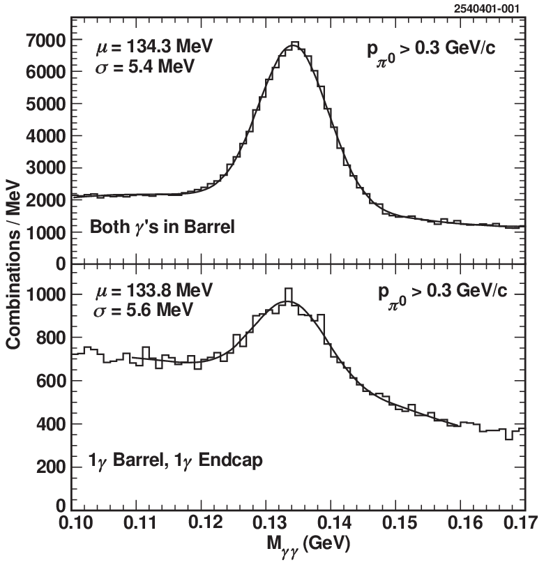
The material from which the crystals were made, CsI, has high density (4.53 g/cm3) and short radiation length (8.93 g/cm3), so it can stop photons and electrons effectively. In the calorimeter, electrons produce photons by Bremsstrahlung and photons undergo production near high- nuclei. This process produces a cascade called an electromagnetic shower. The final low-energy electrons and positrons that result from this shower process excite atoms in the crystals which then “scintillate,” emitting visible light (560 nm) as they return to the ground state. The crystals are transparent for these visible light photons and they are read out using four 1 cm 1 cm photodiodes mounted on the backs of the crystals. Muons and noninteracting hadrons are called minimum ionizing particles (MIPS) as they only deposit a small fraction of their energy by ionization.
The shower reconstruction process starts with calculating the energy deposited in a crystal from the amount of light detected. As the energy of a shower is generally deposited into multiple crystals, a cluster of several adjacent and near-adjacent crystals are considered together. Since including crystals with very small energy deposits can degrade the measurement by bringing in excessive noise, the number of blocks used has been optimized for the best precision. The uncertainty in the energy of the shower is calculated based on energy-weighted average of the blocks in the sum of the cluster, and an example optimization is shown in Figure 15. The number of crystals used is logarithmic in energy and ranges from 4 at 25 MeV to 17 at 4 GeV [58].

The photon energy resolution of CLEO-c calorimeter is about 4.0% at 0.1 GeV and 2.2% at 1 GeV and the angular resolution is approximately 10 mrad. The performance of the endcap region is not as good as that of barrel region because of the presence of the aluminum DR endplates and electronics in front of the crystals. The excellent energy and angular resolution of the calorimeter is critical for the reconstruction of the decay modes that include or decays, as well as the low-energy transition photons in radiative decays.
6.5 Superconducting Magnet
Right outside of the calorimeter is the superconducting solenoid, which has an inner diameter of 3 m and a length of 3.5 m. It provides a uniform (to ) 1-T magnetic field parallel to the beam line over the full volume of the tracking system, the RICH detector and the calorimeter. The solenoid is cooled down to superconducting temperatures by liquid helium. Three layers of 36 cm thick iron flux return for the magnet also serve as part of the absorber for the muon identification system. The magnetic field used to be set at 1.5 T for CLEO III running at a center-of-mass energy of 10.5 GeV. In CLEO-c the center of mass energy is much lower and the momentum of charged particles is much smaller. From Equation 19, one can see that in order to keep the same radius of the curvature for the trajectory of particle, if the momentum of the particle decreases, the magnetic field has to be reduced to allow the tracks to reach the RICH detector and calorimeter.
6.6 Muon Detector
Muons are distinguished from other charged particles by their low probability of interaction as they pass through material. The Muon Detector (MU) is located at the outside of CLEO-c beyond a roughly 1-m steel absorber. The absorber absorbs other particles that pass through the calorimeter, so the hits in the MU chambers are almost exclusively from muons. The muon chambers (MU) operate in the similar way the tracking chambers do. A cross-section view of the muon super-layer is shown in Figure 16.

The muon detector uses gas-filled tracking chambers in between 36 cm iron absorbers surrounding the detector. It consists of three layers of proportional wire chambers of 4 m long, 8.3 cm wide, and 1.0 cm tall and oriented with its long axis parallel to the z-axis.
The muon detector provides the information in terms of interaction length. The interaction lengths (also known as the absorption length) is defined as the mean distance over which a particle travels before scattering inelastically from a nucleus. The barrel super layers are located at depths of 3, 5, and 7 interaction lengths, while the only super-layer in each endcap is located at a depth of about 7 interaction lengths.
The MU is designed to detect muons with momentum of 0.8 Gev or higher. It is not as useful for CLEO-c as it was for the previous experiment because of the much lower center of mass energies.
6.7 Triggers and Data Acquisition System
The trigger and data acquisition (DAQ) systems of CLEO-c are used to collect and process the data from all components of the detector, and save the data to mass storage devices. During CLEO-c runs, interactions happened at the frequency in the order of 1 MHz. The recording capability of the data acquisition system does not allow every collision to be recorded, and most of these interactions are of no interest. The actual rate of interesting physics events is only on the order of 1 Hz. The trigger system, as illustrated in Figure 17, is used to decide whether an event should be recorded based on the complicated information from many components of the detector.

6.7.1 Trigger System
The trigger system is operated in several levels [56, 64, 65, 66]. The first level of trigger, called level-zero (L0), is the hardware trigger. The tracking trigger, including axial and stereo tracking, and calorimeter trigger, including analog and digital calorimeter trigger, both belong to L0. Data from the drift chamber and calorimeter are received and processed in separate VME crates using the appropriate circuit boards to yield initial trigger parameters, such as track count and topology in the drift chamber, and shower count and topology in the electromagnetic calorimeter. The next level trigger is the global level-one (L1) trigger, which correlates the information from both tracking and calorimeter systems. The global trigger circuit generates an L1Pass strobe every time a valid trigger condition is satisfied. The generated L1Pass signals are conditionally transferred to the gating and calibration modules and then distributed to the data acquisition system. The L1 Decision and Data Flow Control system makes a trigger decision every 42 ns based on the information from the tracking system and calorimeter. Programmable trigger decision boards (L1TR), which can be configured for a wide range of topologies, are used to look at this information and respond to various trigger conditions. It takes the tracking system about 2 s and calorimetry over 2.5 s to deliver information for the decision. There are currently about eight trigger lines, which definitions and relative rates are shown in Table 6. The total trigger rate at a luminosity of is between 80 and 90 Hz [56].
| Name | Definition | Relative Rate |
| Hadronic | number of axial track & | 0.41 |
| number of showers below a min. energy | ||
| -pair | back-to-back stereo tracks | 1.40 |
| Barrel Bhabha | back-to-back high showers in CB | 1.0 |
| Endcap Bhabha | back-to-back high showers in CE | 0.23 |
| electron+track | number of axial track & | 1.48 |
| number of showers above a min. energy | ||
| tau/radiative | number of stereo track & | 2 |
| number of showers below a min. energy | ||
| Two Track | number of axial track | 0.69 |
| Random | random 1 kHz source | 1 |
The final trigger stage is called level-three (L3). It is a software trigger, which is implemented on a fast workstation. It takes an event passed by the lower level triggers and either rejects or accepts it based on more sophisticated reconstruction algorithms. Events such as those from cosmic rays or interactions of the beam with residual gas molecules in the beam pipe are rejected by L3 before they are permanently recorded.
6.7.2 Data Acquisition System
The data acquisition system consists of two equally important parts [56]. Data quality and the detector performance are monitored by the slow control system, and the data collection system is responsible for the data transfer from the front end electronics to the mass storage device. The slow control and monitoring system is required to provide sufficient flexibility for online data quality and detector performance monitoring. It also includes run control, alarm and message handling, and calibration constants management. For the data collection system the knowledge of cross sections of the interesting physics processes and expected CESR luminosity are needed to establish the performance requirement. The key parameters for the DAQ system are the expected trigger rate, the acceptable detector dead-time and the average event size. In the current configuration the data acquisition system can operate at trigger rates up to 150 Hz, significantly below the design rate of 1000 Hz. A read-out time, defined as the time between the trigger signal and the end of the digitization process in the front-end electronic modules, causes dead-time and therefore should be kept minimal. The detector dead-time is less than 3% when the average read-out time is 20-30 s at a trigger rate of 1000 Hz.
The structure of the data acquisition system is shown in Figure 18.

For each event that is accepted by the trigger, all detector channels need to be digitized. Front-end data conversion is performed in parallel and local buffers on each data-board hold the data for later asynchronous readout by the data acquisition system. Data sparsification (the suppression of channels without valid hits) is performed directly on the data-boards. The Data-Mover, a dedicated module in each front-end crate, assures transfer times below 500 s and provides a second buffer level. About 30 front-end crates are needed for the detector. The data is sent to L3 and the L3 decision is sent back to the front-end crates. The fragments of the events that are accepted by L3 are transmitted from the crates to the Event-Builder by the Data-Mover. Completely reconstructed events are transferred to the mass storage device and a fraction of the data is analyzed online by a monitor program to quickly discover problems of the detector and to ensure the quality of the stored data.
7 Event Reconstruction
Before the data can be used for physics analyses, the raw data collected needs to be processed by software packages to reconstruct tracks and showers. Raw data collected from different components of the detector are processed through Pass1 and Pass2, which consist of collections of processors and routines for event reconstruction. The detailed processes of the track and shower reconstruction have been described in Sections 6.2.4 and 6.4.
The function of Pass1 is to perform fast classification of the raw data events. It runs online to provide real-time feedback about the performance of the detector while taking data for data quality control. Only one-tenth of the collected events are processed with fast reconstruction. Pass2 processes all events offline and it provides more detailed and accurate event reconstruction. After Pass2 the data are ready for the physics analyses and one can access the data with personal computer program written with a computer language like C++.
8 Monte Carlo Simulation
Monte Carlo (MC) techniques allow the simulation of the data based on the best knowledge of physics properties, detector configuration and detector performance. The simulated data are used to determine detection efficiencies, estimate backgrounds, or determine background and signal shapes for specific physical processes studied, including in this dissertation.
The CLEO-c MC production [67, 68] starts with the generation of a list of particles. In this stage, for example, events are generated with the software package EvtGen [67] and final state radiation (FSR) is simulated with PHOTOS [69]. EvtGen produces Monte Carlo events with a list of particles (and their four-momenta) created in an interaction at a desired energy. In addition to specific states like , it simulates events for where can be an up, down, strange, or charm quark. The quark fragmentation simulation uses an interface to the JetSet software package [70, 71] that models quark and gluon hadronization. The subsequent decays of unstable particles are simulated based on the amplitudes, which are used to calculate the probability for any decay tree from a decay table that is updated periodically to reflect our best knowledge.
The CLEOg is the simulation program based on the GEANT3 [72] package developed at CERN. CLEOg simulates the passage of particles through the CLEO-c detector material and detector elements. At each step, a random number is generated to determine if the particle interacts with any material. If it does, more random numbers are generated to determine its effect on the particle and still more to calculate the signal that would result in the detector element. Using calibration data or samples of data events taken with a random trigger, the detector noise and the beam-related backgrounds are also simulated when no colliding physics events were present. Finally, the simulated events are saved in the same format as raw data so they are processed with the same reconstruction program Pass2.
Chapter \thechapter Measurement of
In this chapter, the analysis of the process of is described in detail. As the channel had never been accurately measured before, I start by introducing the strategy and procedures of this analysis, followed by describing the samples used and the event selection criteria. The study of decays is presented to justify the analysis procedures of decays in Section 13. Finally the results of decays and systematic uncertainty studies are presented.
9 Strategy and Procedures
The analysis was initiated from the CLEO exclusive study of , which was included in the search for [73, 74]. We reconstruct candidates and extract information from the energy of the transition photons.
Various modes have been searched. We constructed an extensive list of possible decay modes following the model of a CLEO-c analysis of [75]. We considered modes with relatively high yields, and selected the following final states: , , , , , with or , with , with or , , , and .
The major challenge of this analysis is to detect the low energy transition photon while suppressing backgrounds. We reconstruct the events exclusively by considering all combinations of charged tracks and photons, and remove the possible candidates of other decays by applying various mode dependent cuts, as described in Section 11. Signal-squared over signal-plus-background [] studies were used to optimize selection criteria for the 4-C kinematic fit and the distance to the nearest track for the transition photon and the angle between the transition photon and the closest track.
Some other modes have been considered but were not included in the final analysis. The modes with large decay branching fractions are expected to have large backgrounds. These modes include and . In addition to these two modes, the following modes are not considered because of high background level based on studies of generic Monte Carlo (MC): , . The modes , , are not considered due to poor signal-to-background ratio based on small expected yields from extrapolating the partial widths from the to the . Modes and are excluded because signal MC studies show they have low efficiency. When optimizing the cuts for the considered modes, the branching fraction of each mode was arbitrarily assumed to be 1% because there are no previous measurements that can provide reliable estimates.
10 Samples
10.1 Data
In order to search for , CLEO-c Datasets 32 and 42 were used. Dataset 32 has 1.44 million decays and Dataset 42 has 24.45 million, giving a total for the CLEO-c data sample of 25.89 million decays [76]. For our final processing we selected a recent update of the CLEO-c software that allowed us to use updated endcap calorimeter (CC) calibrations and a new CC energy-correction procedure (CCFIX) [77].
10.2 Generic Monte Carlo
The 5 times luminosity generic and the 5 times luminosity continuum MC samples, both of which were generated by the Minnesota MC farm, were used for cut optimization and background suppression. The full 10 times generic and continuum MC samples were used for fitting the measured photon energy distribution in the signal region. The new 5 times luminosity generic sample is found to be consistent with that of the original 5 times luminosity sample for this study.
10.3 Signal Monte Carlo
The signal MC sample consists of one million events, distributed over 15 modes, including the 13 modes that were used in this study. (We count the modes with an decay as two separate modes, although they are combined for final measurements.) The sample was generated to replicate the full CLEO-c data sample. The mass () and width () were taken from the PDG [7]. This MC sample was generated using the appropriate angular distribution for a vector to vector-pseudoscalar decay, i.e., , where is the angle between the M1 transition photon and the positron beam. The angular distributions for the decays were thrown according to phase space. The minimum hadronic mass of the was decreased from its default value of 20 MeV below the nominal mass of (3638 MeV) to 210 MeV below in order to appropriately model the tails of the decay.
A signal MC sample to study the decaying to the same hadronic final states was also generated. The study of decays was used to validate the analysis procedure. A one million event sample, distributed over the same modes, was generated. This MC sample was generated using the appropriate angular distribution for a vector to axial vector-pseudoscalar decay, i.e., [78]. As with the signal MC sample, this sample was generated to replicate the full CLEO-c data sample. The mass () and width () [7] were used. The minimum hadronic mass of the was decreased from its default value of 6.0 MeV below the nominal mass of () to 41.6 MeV below in order to appropriately model the tails of the decay.
The numbers of generated events for both and decays are listed in Table 7.
| Mode | ||
|---|---|---|
| 62616 | 71388 | |
| 63103 | 71444 | |
| 62649 | 71659 | |
| 71112 | 71248 | |
| 73383 | 70853 | |
| 71052 | 71904 | |
| 70928 | 71307 | |
| 70986 | 49970 | |
| 70879 | 71145 | |
| 71261 | 71295 | |
| 62972 | 71742 | |
| 62426 | 70908 | |
| 64556 | 71063 |
11 Event Selection
It was required that the net charge of the event equal zero and the number of good tracks match the number of charged tracks in the decay mode.
11.1 Track Selection
We used standard CLEO-c selection criteria for track quality and particle identification (PID). These have been developed for use in high-precision measurements of decays by the CLEO-c “DTag” subgroup [79]. They are applied in selecting ’s and ’s.
11.1.1 Track Quality
For track quality, it was required that the track have a successful Kalman fit. Also the projection of the distance from the interaction point of the annihilation (IP) to the origin of the track on the plane and the projection of the distance between the IP and origin of the track along the -axis were required for each qualified track, with exception of charged tracks from decays. (If charged tracks are daughters of a , the and of the track tend to be larger as the charged particles are created at where the decays rather than the IP.)
11.1.2 Particle ID
The Particle ID criteria developed by the DTag group were used for charged pions and kaons. Those criteria are
- •
, where is the angle between the initial momentum of the track and the direction of the beam, the axis
- •
RICH information is valid
- •
Both , hypotheses analyzed
- •
consistency with the or hypothesis, which means if the distribution for the or hypothesis is Gaussian, then
where and are the mean and standard deviation of the the distribution for the or hypothesis
- •
If the momentum of the particle is greater than or equal to :
-
More than two photons on the Cherenkov ring (See Section 6.3) are associated to the pion or kaon
-
Combined log-likelihood for , for , where and are the log-likelihoods for the and hypothesis, respectively, and and are the standard deviation of the distribution for the and hypothesis as defined above as
-
- •
If the momentum of the particle is smaller than , or if RICH information is not available: for , for
For any mode including a pair, only one kaon is required to pass the PID to increase the efficiency.
11.2 Photon Selection
General requirements for selecting photons, both from radiative transitions and in reconstruction, were applied. We required that a shower does not contain any “hot” crystals, is not matched to the projection of a charged track into the CC, and has E9/E25 OK. E9/E25 is the ratio between the total energy from 9 central crystals around the highest energy crystal and the total energy from the 25 crystals centering at the highest energy crystal in the calorimeter. E9/E25 OK means that for a shower with a certain energy, the ratio is within 99% of the E9/E25 photon like distribution at this energy.
In selecting candidate transition photons for the decay , we required the energy to be in the range . Because of the degraded photon resolution and efficiency in the endcap, we selected showers in the good barrel only, .
11.3 Selection
We required the flight significance to be greater than 3. flight significance is the ratio of the distance between the position of where it decays to two charged tracks and the beam spot to the measurement error of the position determined by the error matrix. In another word, the intersection of the two charged tracks that are daughters was required to be far enough from the interaction point.
The mass of a candidates was required to be within of the nominal mass, i.e., .
11.4 Neutral Pion Selection
For selecting photons used to compose a or , CLEO-c software PhotonDecaysProd was used with the following defaults for the CLEO-c software packages NavPi0ToGG and NavEtaToGG: E9/E25 OK, unmatched shower in good barrel or good endcap, and .
candidates were obtained from the table of candidates that was produced by NavPi0toGG. The default photon energy threshold of NavPi0ToGG table is 30 MeV in the good barrel and 50 MeV elsewhere. No hot crystals and E9/E25 OK were also required. The only additional requirement for selecting ’s was to require the pull mass of the to be within . The pull mass is defined as the ratio of the difference between the mass of the candidate and the nominal mass divided by the standard deviation of the mass distribution. This means that the mass of the candidate was required to be close enough to the nominal mass.
11.5 Selection
The candidates were reconstructed in two ways, and .
The candidates were obtained from the NavEtaToGG (CLEO-c software package) table similar to selecting the candidates. The default requirements of photons in NavEtaToGG are the same as NavPi0ToGG. Similarly, the only additional requirement for selecting decays was to require the pull mass of the to be within .
For , we required the mass of combination to be within of the nominal mass, i.e., . Figure 19 shows simulated mass distributions before the cut was applied in the two modes with .


11.6 selection
Among the seven modes we considered, only one mode has an decay, , . For this mode we required the invariant mass of the hadrons that compose the to be within of the expected mass, . Figure 20 shows simulated mass distributions for this mode before the cut was applied.

11.7 Suppression of Background Charmonium States
In following section, we describe selection criteria used to suppress production of other charmonium states observed in the generic MC samples.
11.7.1 Hadronic Invariant Mass Difference
To suppress decays of direct and , produced via , to the hadronic final states under investigation, we require the hadronic invariant mass difference to be in the range [0,100] MeV, where is the PDG value of the mass [7], and is the reconstructed hadronic invariant mass.
11.7.2 Recoil Mass
In selecting decays to final states with an decay, large backgrounds arise from decays. The branching fraction of this decay mode is [7]. Therefore we applied recoil mass cuts to the modes and . In the mode , , although an is in the decay, we did not apply the recoil mass cut because the selection of has already eliminated .
The recoil mass cut was mode dependent. For mode , we rejected events with the recoil mass within of the mass by requiring . For mode , we required . Simulated recoil mass distributions before applying this cut are shown in Figure 21. These cuts were found to be unnecessary for the and modes.


11.7.3 Photon Recoil Mass
In modes that contain and decays, a large amount of background comes from using the photon from the decay with another photon. By applying mode dependent recoil mass cuts, we effectively remove a large amount of this background.
For modes and , since MeV [7], a relatively large mass compared to the energy of the transition photons in the decays (100-300 MeV), the transition photon is sometimes used as the low energy photon in the decay. Therefore we examined the photon recoil mass for the lower energy photon in decays. For these two modes, we rejected events by requiring
- •
- •
- •
For the mode , since MeV [7], a relatively small mass compared to the energy of the transition photon (100-300 MeV), the high energy photon is more likely swapped with the transition photon. Therefore we examined the photon recoil mass for the higher energy photon in decays. For this mode, we rejected events by requiring
- •
- •
- •
Similar to the case of the recoil mass cut, modes and , even though they contain decays, the photons used to form the candidate did not contain contamination from decays. Therefore no photon recoil mass cut was applied to these two modes.
Figures 22 and 23 show the simulated distributions of photon recoil mass for the decay modes , , and before applying these cuts.


11.7.4 Rejection - Recoil Mass
For the modes that include charged pion pairs, we rejected events which contained decays of . Specifically, we required for modes , , , , and , and for mode . With these requirements, we can suppress background from the decay , which is a dominant decay mode of ().
The distributions of recoil mass for modes , , , , , before applying this cut are shown in Figures 24 through 26.


11.7.5 Rejection - Hadron Invariant Mass
Even after we rejected events with the recoil mass cuts, decays, where is a particular final state under study, were still observed in the generic MC sample. This background can be further suppressed by requiring the invariant mass of hadrons (excluding the pair) to be displaced from the mass. More specifically, for the modes = , , , , , we reject events by requiring .
Figure 27 shows the distributions of hadron invariant mass for the mode before applying the cut. The distributions for other four modes (, , , and ) before applying the cut are shown in Figure 28.


11.8 Photon Background Suppression
We investigated background suppression strategies related to the relationship between the candidate transition photon and the charged tracks in the event.
Photons which are emitted from charged particles are typically in the same direction as the initial momentum vector of the charged particle at the IP. These photons are called final state radiation (FSR). If a shower is close to a nearby track in the CC, it may be a splitoff shower (a shower that split off from a hadronic interaction of a nearby track in the CC). To identify and remove these backgrounds, the angle between the transition photon and the initial momentum of the closest pion () and the distance between the transition photon and the nearest track () were studied. Although either of these can help remove FSR and splitoff showers, a cut on the angle between the transition photon and the initial momentum of the closest pion is more efficient in suppressing final state radiation and a cut on the distance between the transition photon and the nearest track is more efficient in removing splitoff showers. In this analysis, the following rules were applied while making the decision on which of these two cuts would be applied to a mode:
- •
If the hadronic decay only contained charged pions, cut on the angle between the initial pion momentum and the candidate transition photon.
- •
If the hadronic decay only contained charged kaons, cut on the distance of the closest track to the candidate transition photon.
- •
If the hadronic decay contained both charged pions and kaons, cut on the distance of the closest track to the candidate transition photon, then we examined if a cut on the angle between initial pion momentum and the candidate transition photon improves the . (We did not apply both types of cuts to the same mode.)
We optimized the selection criteria by evaluating the figure of merit at different cut values. The value of was from the signal MC sample with the assumption that for all decay modes. The value of was from the sum of the 5 times generic and continuum MC samples scaled to the true luminosity of data. The plot of versus cut value was examined to determine the optimal cut value. An example of the is shown in Figure 29 for the mode. The for the other modes are shown in Figures 30 through 32. The optimized cut for each mode is listed in Table 8.


11.9 Global Event Selection
11.9.1 4-Constraint Kinematic Fit dof
To select events consistent with full detection of we compute the 4-constraint kinematic fit using the package FitEvt [80] . Both momentum and vertex constraints were imposed. For each mode, a vertex fit of the charged tracks from the IP was performed first and the fit result was used as the origin of the photon(s) in the kinematic fit. In the fit we imposed the constraint that the total 4-momentum of all tracks and neutral particles be equal to the total 4-momentum of the . We optimized a cut on the resulting overall in the same manner as the optimization of the cuts on nearby tracks (see Section 11.8), using as the figure of merit. An example of the optimization for the 4-momentum kinematic fit is shown in Figure 33 for the mode. The for the other modes are shown in Figures 34 through 36. The optimized cuts are listed in Table 8.
| Mode | (cm) or | |
|---|---|---|
| - | ||
| - | ||
| - | ||
| - | ||
| - | ||
| - | ||
| - | ||
| - | ||
| - |


11.9.2 4-Constraint Kinematic Fit dof of Hadrons Only
Similar to the 4-constraint kinematic fit for the whole event, we used the FitEvt package [80] to perform the fit only for the hadrons of candidates, both momentum and vertex. In the fit we impose the constraint that the total 4-momentum of all hadrons be equal to the total 4-momentum of the . If a candidate is a event, then the 4-C kinematic fit of the whole event should peak at zero, and that of just the hadrons should be distributed away from zero. This cut was evaluated, but was found not to suppress the background as efficiently as hoped. Therefore it was excluded from the final set of selection criteria.
12 Signal Extraction Procedures
In this section, we describe the procedure we developed for extracting the signal yields and resonance parameters from the 25.9 M decays. We fit the measured, or unconstrained, photon energy distribution in the range . Figure 37 shows the expected signal distribution for the modes and for a mock data sample of 25.9 M decays generated under the assumption that the partial widths for are the same as for , and .


12.1 Detector Resolution
Since we extract the signal from a measured photon distribution, a Crystal Ball function [81, 82] is used to fit the detector resolution distribution from the signal MC samples described in Section 10.3. The Crystal Ball function (named for the Crystal Ball experiment) is designed to provide a good representation of the photon energy distribution as measured with a high-precision crystal calorimeter like CLEO-c’s. The resolution is defined as the standard deviation of the difference between the measured and generator-level photon energy. The RooFit software package [83] was used to perform these fits.
The Crystal Ball function is defined as
| (23) |
where is the normalization factor and , , , and are parameters that govern the shape. The parameter represents the mean of the resolution function and is the resolution in the photon energy. The Crystal Ball function features a Gaussian distribution with a power-law tail (index ) at the low end below a threshold (given by the parameter ) to account for energy leakage within the calorimeter.
To obtain successful fits for the resolution function, the parameter was fixed at 140 for all modes. It was observed that when varied over the range from 40 to 140, the shape of the Crystal Ball function and the fit showed very little variation.
As an example Figure 38 shows the resolution fit of the mode. Resolution fits of other modes are shown in Appendix Study of Radiative Decays of Psi(2S) Mesons.

12.2 Background Parametrization
A necessary ingredient for obtaining reliable results was the use of an appropriate function to describe the background shape. For this purpose we can either use a polynomial or other function to parametrize the background or rely on a MC simulation that at least approximates the underlying physics. Clearly the latter is potentially more reliable, but it is first necessary to study the reliability of our MC samples and the composition of the background. An independent data sample is required for such a study, and we used events with four specific decay modes. These modes are , , , and . Note that these modes gave us a sample of decays modes with and . When selecting events, the recoil mass was required to be within 20 MeV of the mass of . All other event selection criteria for decays were applied, except that the recoil mass and rejection cuts were removed and the hadronic invariant mass cut was adjusted for the mass instead of the mass of .


The two primary sources of low energy shower backgrounds are splitoff showers and FSR. The splitoff showers are generally very close to the track associated with them. Most splitoff showers are removed by the cut on the transition photon candidate distance to the nearest track, but some pass through the cut. Additional splitoff showers can be removed with a tighter cut on the full event 4-constraint kinematic fit . Figure 39 shows the fits of the measured photon energy distribution for data in decays with an accompanying (background) photon candidate. The upper left plot in the figure shows a fit using the 5 times luminosity generic and continuum MC samples with one free parameter (normalization) for the background. The upper right plot shows a two parameter fit to the separate distributions for non-splitoff showers (mostly FSR) and for splitoff showers. A shower was MC-truth tagged as a splitoff shower if its parent was not a photon. (”MC-truth tagging” uses detailed information stored at the time the MC was created to select only those particles that come from a particular process.) The lower left plot shows a histogram (one parameter) fit for events when the 4-constraint kinematic fit has been tightened to be less than 3. The lower right plot shows a fit with a linear background function. Figures 40 through 42 show similar plots for the other three decay modes. The fits show that the low energy shower distribution of the background MC sample represents the data quite well. Fitting with the two sources of backgrounds separately does not lead to obvious improvement of background fitting based on the resulting . Table 9 shows the results of the four types of fits for all four decay modes studied.
| Mode | 1 hist | 2 hist | tight | linear |
|---|---|---|---|---|
| 1.25 | 1.31 | 1.92 | 1.27 | |
| 0.59 | 0.61 | 0.74 | 0.99 | |
| 0.59 | 0.52 | 0.96 | 0.99 | |
| 1.99 | 2.05 | 1.79 | 2.48 | |
This study showed that a linear background function provides a reasonable alternative to the MC-predicted distributions but one that is not based on the physics of decays or the CLEO-c detector. Based on this investigation, we chose the single-histogram as our standard background shape fit in studying the , decays. The linear fit is included as an alternative for evaluating the systematic uncertainty in the fits.
12.3 Signal Fit
The measured, or unconstrained, shower energy distribution was fit for a signal using a non-relativistic Breit-Wigner function (Cauchy distribution) [84, 85] convolved with the Crystal Ball resolution function. The parameters of the Crystal Ball function, , , and were obtained from the resolution fit and were fixed in the signal fits. The Breit-Wigner function is defined as follows:
| (24) |
where is the width of the resonance and is the mean of the variable . In our signal fits, represents the measured photon energy.
For the signal fits, the parameters are extracted with a binned likelihood fit, minimizing the negative logarithm of likelihood using RooFit [83]. For each mode the histogram background shape was the sum of events from the 10 times generic and 5 times continuum MC sample which passed our selection criteria. We fit the data with the above signal function and background histogram.
To verify the fitting procedure, the decays of were studied. The details of this study can be found in Section 13.
13 Test of Fit Procedure with Decays
The study of the decay channel was used to verify the analysis procedures for the decay .
13.1 Introduction
The radiative decay of is similar to the decay . The is the P-wave spin triplet charmonium state with total angular momentum mass MeV, and width MeV [7]. For a meson nearly at rest, the transition photon from the decay should have energy around MeV. This is 80 MeV higher than the energy of the transition photon in the decay . While the photon energy range and background parametrization for the study are different from the study, the other event features and analysis procedures are very similar.
13.2 Analysis Procedures
Since the purpose of studying this decay channel is to evaluate the analysis procedure of , similar procedures were applied to decays. The results were obtained from similar resolution and signal fits on signal MC and data samples.
Same as decays, the data sample for this study was the full sample of Data 32 and Data 42 of CLEO-c data, 25.9 M decays. As described in Section 10.3, the signal MC sample was generated to replicate the full CLEO-c sample, similar to the sample.
To validate the event selection criteria for decays, the same criteria for decays were applied to decays, except that was removed and was replaced with .
13.3 Results
For each mode, the Crystal Ball function [82] was used to determine the detector resolution of the measured photon energy from signal MC. The parameter of the Crystal Ball function was set at a fixed value of in order to obtain successful fits. From the resolution fits, the value of and were determined. These values were then fixed and applied in fitting the measured photon energy distribution of data.
In the signal fit of each mode, we used a Breit-Wigner distribution convolved with a Crystal Ball resolution as the signal function. In addition to fixed , and , the width () was fixed to MeV. Unlike the study, the background shape was either a linear function, constant, or no background, depending on the fitting status of the linear background fit. For all modes, a fit with a linear background and mean left free was performed first. If the linear fit did not converge, and the signal mean was within of the nominal mean (127.60 MeV), then a fit with a constant background and mean left free was attempted. If the linear fit did not converge and the mean was not within of the nominal value, then a fit with a constant background and the mean fixed to 127.60 MeV was attempted. If the linear fit resulted in a background with a negative yield, then a fit with no background was performed. According to these rules, the modes , , , and were fit with a linear background; the modes , , and were fit with a constant background; the modes and with were fit with a constant background and fixed mean; and the modes and were fit without a background.
The efficiencies and the resolution fit results are listed in Table 10. The branching fractions of the decays are given by
| (25) |
where is the number of signal events (yields) determined by the signal fits, is the efficiency, is the total number of decays, and is the branching fraction of . When calculating the branching fractions of , we used [76] and [7]. The results of the signal fits and the corresponding branching fractions are listed in Table 11. The data fits for all thirteen modes are shown in Figures 43 through 49, while the resolution fits are shown in Appendix Study of Radiative Decays of Psi(2S) Mesons.
| Mode | (%) | Res (MeV) | XBall |
|---|---|---|---|
| Mode | Mean (MeV) | () | () | |
|---|---|---|---|---|
| - | ||||
| - | ||||
| - |


13.4 Discussion and Conclusion for the Study
From the results we can see that for most modes the results are consistent with the world averages. However, two modes show inconsistency with the PDG values, and .
The previous CLEO measurement [87, 88] shows the result of the branching fractions of decays to be for mode, for mode, for mode, and for mode. Our results are consistent with this measurement except for mode. The cuts in our measurements are not optimized for studies.
The PDG branching fraction average for is dominated by measurement from the BES-I collaboration [89]. As can be seen in Table 12, the BES-I results are systematically lower than our results, while our measurement of is completely consistent with the PDG average.
| Mode | PDG | This result | BES-I | This Result/BES-I |
|---|---|---|---|---|
For the mode ,we were not able to explain for the discrepancy other than a statistical fluctuation in either our or the previous CLEO measurement [87, 88].
Some of the decay modes like , and have not been measured before. For the decay mode , only upper limits were given in PDG based on previous measurements. In this study, the branching fractions of to these modes were determined. Even though the decays were studied with the optimized criteria for decays, the branching fractions results are consistent with values listed by the PDG. If the decays were studied with the optimized criteria for decays, the efficiencies would have been higher and the statistical error would have been reduced.
Overall, the results of the study of , decays establish the validity of the analysis procedures for . There is no explanation for the small, but statistically significant, discrepancy observed in the mode, but since the analysis of this mode is not appreciably different from the higher-statistics modes, we assume that it too has no fundamental flaw.
14 Results for
The measured photon energy results for the signal region are listed in Table 13. The resolution function fits are shown in Appendix Study of Radiative Decays of Psi(2S) Mesons and the corresponding values for and are fixed in the fits of the data sample. The resonance parameters () and are also fixed in the fits. The photon energy distributions for all eleven modes are shown in Figures 50 through 54.


Two methods are employed for determining the 90% confidence level upper limits on the yields listed in Table 13. For modes which do not contain decays, we have no apparent signals and substantial backgrounds. Therefore, we determine an upper limit by integrating the distribution defined from the nominal yield result (a bifurcated Gaussian) up to 90% of the area in the positive physical range. We use toy MC studies to verify that we get consistent results with the nominal fit integration. For modes with decays, a very limited number of events pass our selection criteria, either signal or background. Therefore, we use the Feldman and Cousins method [90]. The procedure of determining the upper limits is described in more detail in Appendix Study of Radiative Decays of Psi(2S) Mesons.
| Mode | Res | XBall | Sgnf | ||||
|---|---|---|---|---|---|---|---|
| () | (%) | (MeV) | () | () | |||
| * | |||||||
| * | – | – | – | ||||
| – | – | – | |||||
| * | – | – | – | ||||
| – | |||||||
*Submode-decay branching fractions are included in efficiencies.
The modes and are actually specific final states of . Therefore, we also determined the product branching fraction for the decay . Figure 55 shows the fit result of the combined final states. The results are also listed in Table 13.
The statistical significance, defined as , where is is the likelihood and the difference is computed between the standard fit with both signal and background and an alternative background-only fit. Excluding the mode, the product of branching fractions ( in Table 13) was obtained from
| (26) |
where is the number of signal events (yields) determined by fits for non- modes and Feldman-Cousins table for modes contain ’s, is the efficiency, is the total number of decays. For mode additional factors of and should be considered and the corresponding equation becomes
| (27) |
When calculating the upper limits of the branching fraction product we used [76]. The results of the upper limits of branching fraction products at 90% confidence level are also listed in Table 13.
No evidence for the decay is observed in any of the these modes. The only mode in which an excess above background is present with a statistical significance greater than 2 is the 4 mode. We have investigated other aspects of the events in the signal region to determine if the excess constitutes evidence of a signal or is just a statistical fluctuation.
Figure 56 shows the distribution of the photon for the 4 mode. The points are determined by the measured photon energy yields after requiring the photon candidate to be within a given region. This distribution is fit to the expected dependence, giving a of 3.7/2, which corresponds to a confidence level of only 16%.
Another test was to fit the distribution in the constrained photon energy, the value returned by the 4C kinematic fit to the , hypothesis. If the events in the excess are true signal, we would expect the significance to be increased. In fact it is reduced to only . Figure 57 displays the constrained photon energy for the mode.
These tests suggest that the excess of events in the signal region for the mode is caused by an upward fluctuation of the background rather than true signal.


Our conclusion is that there is no statistically significant excess attributable to in any of the 11 modes considered. It is reasonable to ask whether the sum over all exclusive modes shows evidence of an excess, even though the interpretation of such an excess would be complicated. Figure 58 (top) shows the measured photon energy distribution summed over all 11 modes (points). It can be compared with a “background-only” hypothesis constructed as the sum of the distributions from mode-by-mode fits to the MC-determined background histograms with no signal component included (solid histogram). A small excess is visible in the signal region, but it is clearly not statistically significant.
Figure 58 (top) shows a clear discrepancy between the fitted background and the observed yield in the lowest photon-energy bins. As was discussed previously, this region has a significant contribution from splitoff showers. In our study (Figure 39 through 42), we tested the reliability of the background simulation in events that are similar to signal events. In addition to parameterizing the background with a single MC-predicted distribution, we considered the alternative of fitting to two separated background components: splitoff showers and showers from all other sources. While there was some improvement in fit quality for the fits with two independent background parameters compared to fits with a single background parameter, it was not statistically compelling and we adopted fits with one background parameter for our standard procedure. The discrepancy observed in Figure 58 (top) may demonstrate that for the full set of 11 signal modes the standard MC does not provide a satisfactory description of the background. This led us to reconsider whether fitting with two background parameters would give better agreement.
Figure 58 (bottom) shows the same data points with the summed histogram obtained from background-only fits with two parameters, one controlling the contribution of splitoff showers and one for other showers. The separate background components were constrained to be positive. Because of insufficient statistics to determine a second background parameter, the treatment of the modes was left unmodified. The sum of the background distributions for the modified fits in Figure 58 (bottom) shows clear improvement in the agreement with the data, suggesting a deficiency in the MC that is at least partially addressed by the fits with two background parameters. Our conclusion that there is no statistically significant excess attributable to stands, but this exercise provides a reminder of possible systematic sensitivity in our results to the treatment of the background.


From Figure 58, because of the low statistics, we cannot find an explanation other than statistical fluctuation for the possible discrepancy between data and MC around 70 MeV.
15 Systematic Uncertainties
While no evidence for the transition was observed in any of the 11 modes we studied, systematic uncertainties were evaluated and incorporated into the branching fraction upper limits.
The systematic uncertainties due to various cuts were studied in the following environments. Some systematic uncertainties have been performed in other CLEO analyses, and the others can be estimated by studying decays of or fits. We used , decays to study the selection criteria, although sufficient statistics were available for only six modes of decays: , , , , and . For some other modes, we estimated systematic uncertainties by relating to modes with similar combinations of final state particles, e.g., for the mode we applied the corresponding systematic uncertainties from the studies. We studied the signal region to assess uncertainties in the signal fitting method.
15.1 Systematic Uncertainties That Apply to All Studied Modes
Some of the systematic uncertainties were applied to all modes. The uncertainty on the total number of was 2% [76]. The systematic errors on the trigger, which arise from uncertainties in the efficiency of trigger decisions for different final states, were taken to be 1% for all modes [91, 92]. The systematic error in the efficiency for detecting the transition photon was 2% [91, 92]. The results of mode dependent systematic uncertainties that were determined by studying decays are listed in Table 14, while the results determined by studying the signal region are listed in Table 15.
15.1.1 Global Event Selection Systematics
We conservatively take the respective systematic uncertainties associated with from the full event vertex fit and the from the full event 4C fit to be the difference between the results obtained with and without those cuts applied. An uncertainty of was assigned to the from the full event vertex fit for all modes. For modes without (with) a decay we assigned a () uncertainty due to the from the full event 4C fit. The per mode results can be found in Table 14.
15.1.2 Resolution Function Systematics
Resolution function systematics were studied by individually adjusting the Crystal Ball parameters and by one standard deviation and finding the changes in the results of branching fractions from decays. We also performed the same procedures for the decay candidates and obtained consistent but smaller results. We assigned and systematic uncertainties due to the uncertainties in and , respectively. The per mode results from the study are listed in Table 14.
15.1.3 Signal Region Systematics
We studied the effect of the lower boundary of the signal region through studying decays by increasing the lower boundary of the signal region from to 104-110 MeV, which is about below the mean of the . This amount is the same as the difference between the lower boundary in the signal region and the mean of the . We assigned a systematic uncertainty of to all modes. The per mode results can be found in Table 14.
The systematic uncertainties due to the high side boundary of the signal region were studied directly in the signal region. The changes of the upper limits of branching fraction products were determined by varying the upper boundary of the signal region by . The results can be found in Table 15.
15.1.4 Hadronic Invariant Mass Systematics
The systematics due to the hadronic invariant mass cut were estimated by removing the cut from the decay search and observing the effect it has on the upper limits of branching fraction products. This actually studied the change in the background. The results are listed in Table 15.
We also studied the decays by adding a requirement of to simulate the effect of adding a cut of at the value below to the lower boundary of the signal region. Results are shown in Table 14, and the sensitivity is found to be smaller than in the signal region.
15.1.5 Background Shape Systematics
The systematic uncertainties associated with the background shape were estimated using the signal region. In non- decay modes, the uncertainties were obtained by repeating the signal fits but replacing the histogram background with linear or constant functions. For modes, in which we do not use fits for upper limit estimates, we use the same number of observed events but take the background in the signal region down by , where is the square root of the number of data events in the sideband region. The difference between this and the nominal result was assigned as the systematic uncertainty. The results can be found in Table 15.
| Mode | A | B | C | D | E | |
|---|---|---|---|---|---|---|
| MeV | ||||||
| Mode | A | B | C |
|---|---|---|---|
| – | |||
| – | |||
| – | |||
15.2 Systematic Uncertainties That Apply Only to Specific Modes
Other systematic uncertainties apply to only specific modes. Table 16 shows a summary of these uncertainties.
| Mode | A | B | C | D | E | F | G | H | I | J | K |
|---|---|---|---|---|---|---|---|---|---|---|---|
| 1.2 | 0.8 | - | - | - | - | - | - | - | |||
| 1.8 | 1.2 | - | - | - | - | - | - | - | |||
| 1.8 | 1.0 | - | - | - | - | - | - | ||||
| 1.2 | 0.6 | 3.5 | - | - | - | - | - | - | |||
| 0.9 | 0.5 | - | - | 2 | - | - | - | - | - | - | |
| 0.6 | 0.4 | 3.5 | - | - | - | - | - | - | |||
| 1.2 | 0.8 | 3.5 | - | - | - | - | - | ||||
| 1.2 | 0.8 | 3.5 | - | - | - | - | - | - | - | ||
| 1.2 | 0.6 | 3.5 | - | - | - | - | - | - | - | ||
| 1.8 | 1.0 | 3.5 | - | - | - | - | - | - | - | ||
| 1.8 | 1.0 | 3.5 | - | - | - | - | - | - | |||
| 2.4 | 1.4 | - | - | - | - | - | - | - | |||
| 1.5 | 0.9 | - | - | 2 | - | - | - | - |
15.2.1 Tracking and PID Systematics
For tracking uncertainties we applied 0.3% for pions and 0.6% for kaons based on studies of hadronic decays, which used the full data and standard DTag track quality cuts [93].
Based on the study of the first data [94], the pion (kaon) PID efficiency determined from MC was 0.55% (1.06%) higher than determined from data. Therefore, we decreased the MC-determined efficiencies by these amounts per track. We conservatively assign 0.2% (0.3%) uncertainty to the pion (kaon) PID.
The uncertainties due to the same type of tracks are combined with full correlation. The uncertainties due to different type of tracks are considered uncorrelated, since they are determined through independent studies using specially selected event samples that have minimal overlap with our sample.
15.2.2 and Finding Systematics
The uncertainty for finding was determined by using the results of the finding study which used the full data sample [95].
Our selection criteria are slightly different from the nominal criteria used in that study since we use the CCFIX. The CCFIX makes two types of changes to standard photon reconstruction. It increases the photon resolution in MC by 20% and increases the reported errors of the photon uncertainty in data and MC by 20% [77]. Using the result in Ref. [95] with a loose pull-mass cut of is then similar to using the CCFIX. Defining , the result for with a pull mass and E9/E25 OK cuts applied to the children is . Interestingly, with a pull mass and no E9/E25 OK cuts applied to the children, suggesting the E9/E25 OK cuts do not effect finding.
The uncertainty due to finding was determined based on the studies of decays in the 27.4 M data sample [96]. This study found without the CCFIX but applying the E9/E25 OK cuts, without the CCFIX and the E9/E25 OK cuts, with the CCFIX and without the E9/E25 OK cuts. This suggests that the MC-determined efficiency overestimates the finding efficiency by and that the E9/E25 OK cut does not effect finding.
Based on the interpretations of the studies above, we decreased the MC-determined efficiencies by 3.5% and conservatively assigned systematic uncertainties of 3.5% for both and finding. The systematic uncertainty for decays was determined by applying the assigned and systematic uncertainties. Similarly, the systematic uncertainty for decays were determined by applying the assigned and systematic uncertainties.
15.2.3 Finding Systematics
15.2.4 and Selection Systematics
The uncertainties due to the mass ranges used to select and decays were determined by changing the corresponding or mass ranges to ranges in which the inefficiencies double with respect to our nominal range. These inefficiencies correspond to the mass ranges of for decays and for the mode.
15.2.5 Recoil Mass Systematics
The uncertainties associated with rejection based on the recoil mass criteria were determined by studying , decays with the cuts removed and observing the change of the branching fractions.
15.2.6 Systematics
The uncertainties due to the cut on the hadronic invariant mass determined while excluding a pion pair for rejection were determined based on decays of by removing the cuts and observing the change of the branching fractions.
15.2.7 and Systematics
The systematics due to the cuts on the angle between the momenta of the transition photon and the closest pion (), and the distance between the transition photon and the nearest track () were determined by removing the cut and observing the change of the final results. For the and modes we studied , decays. For and modes, we applied the results from the , decay studies for the and modes, respectively.
15.2.8 Photon Recoil Mass Systematics
The uncertainties associated with the photon recoil mass cuts, which rejects events where the transition photon was used as a child in a reconstructed or decay (), were determined based on the decay of , by applying the cut to this mode and observing the change of the branching fraction. We applied this uncertainty to the , , and modes.
15.2.9 Recoil Mass Systematics
The systematic uncertainties due to the recoil mass cuts (), which were used for rejection, were determined by changing the recoil mass range to double the inefficiency with respect to the nominal cut. These inefficiencies correspond to mass range for the mode and for the mode.
15.3 Summary
Consideration of the full set of systematic uncertainties listed in Tables 14 through 16, as well as those due to the trigger, the number of , and transition photon finding, reveals that the majority of the overall systematic uncertainty is due to the treatment of the background. These factors are listed in Column C of Table 15. The signal region (Column A of Table 15) also shows significant uncertainty associated with the high limit. However, this sensitivity is due to the fact that changing the upper boundary of the signal region changes the background shape because of the low statistics in the region. Therefore, the results listed in Column A of Table 15 are mostly redundant with the background shape uncertainties (Column C of Table 15). Table 17 lists the total systematic uncertainty applied to each mode. In general, the individual uncertainties are treated as uncorrelated and are combined in quadrature to obtain the overall systematic uncertainties in our product branching fraction measurements.
| Mode | Syst Err (%) |
|---|---|
Chapter \thechapter Conclusions and Discussions
16 Summary of Results
We do not observe the transition in any of the decay modes studied. Table 18 lists the results of the product branching fractions using the nominal value of the full width ( [52]). Even though we may have an excess of events in the mode, we did not find any strong evidence for the decay.
| Mode | Corrected | |||
|---|---|---|---|---|
| (90% C.L.) | (%) | (stat only) | (stat+syst) | |
| * | ||||
| * | ||||
| * | ||||
*Submode-decay branching fractions are included in efficiencies.
The effect of the full width uncertainty was determined as follows. Separate signal MC samples with 7 and 21 MeV were generated in the same manner as the nominal MC sample described in Section 10.3. The measured photon energy distributions were fit in the same manner as the nominal procedure, but with the resolution functions determined from these MC samples and the full width of the signal shape adjusted according to the full width being investigated. The results using 7 and 21 MeV, and the linear extrapolation of the product branching fraction as a function of , are listed in Table 18.
| Mode | a | b | ||||||
| (%) | (%) | () | () | |||||
| 7.04 | 0.505 | |||||||
| 3.88 | 0.727 | |||||||
| 3.10 | 0.500 | |||||||
| 2.08 | 0.217 | |||||||
| 2.43 | 0.095 | |||||||
| * | * | 6.48 | 0.542 | |||||
| * | * | 2.95 | 0.095 | |||||
| 10.1 | 0.309 | |||||||
| * | * | 4.08 | 0.127 | |||||
| 14.4 | 1.95 | |||||||
| 4.91 | 0.317 | |||||||
| 8.19 | 0.486 | |||||||
*Submode-decay branching fractions are included in efficiencies.
The branching fractions of may be estimated from branching fractions and the ratio of the full width of the and if the matrix elements governing the decays of the are similar to those of the . Since the studies of built confidence in this analysis procedure, the most likely explanation of the non-observation is that the branching fraction assumptions were overly optimistic. Our original objectives for measuring the resonance properties of the cannot be achieved with this data sample. The upper limits of the branching fractions were obtained instead.
17 Comparison with Published Results
The recent CLEO measurement for requires a reestimate of , as computed using Equation 11 in Section 3.4. Reaveraging , after including the CLEO result of [100], leads to . Using the PDG 2008 values for , , , and [52], along with this new value for , replaces the prediction given in Equation 14 with , which is 50% larger.
The BaBar collaboration recently measured the branching fraction for to be [54], where the first two errors are statistical and systematic, respectively, and the last error is from the measurement of [101]. Using the central value of the BaBar result with our 90% confidence level upper limit of leads to an upper limit of . This limit is roughly twice the revised phenomenological prediction given in the last paragraph.
The BaBar measurement of can also be used to obtain an improved estimate of the two-photon partial width of the . CLEO [47] previously measured the ratio
| (28) | |||||
and assumed equal branching fractions to for and to obtain a first estimate of keV. Using BaBar’s , the PDG value of keV, and % [52], the CLEO measurement of can be reinterpreted to give keV.
A recent analysis from the Belle collaboration found and [55], both at confidence level. Using the result above, these two results give upper limits of and .
Our results for the and modes can be used to determine comparable upper limits. Using leads to upper limits of and . Our upper limit results are an order of magnitude larger than the corresponding upper limits determined from the Belle results.
The branching fraction measurement for and the upper limits for from the Belle collaboration are all lower than predictions made by assuming the partial widths of the these decays are the same as for the . Using the PDG 2008 values for the and full widths, and , and assuming the partial widths for the and decays are identical, leads to all branching fractions being increased by for . Using the PDG 2008 values for the branching fractions , , and , leads to , and , where the last error is from the full width scale factor. The measurement is smaller than the partial width scaling assumption but, after considering the uncertainties, they only differ by . The and upper limit results are and smaller, respectively, but only differ by 1.6 and 1.5 . Higher precision measurements of the full width and are needed in order to determine if the partial width scaling assumption is correct for the states. It should be noted that this may not be true since, for example, we see large differences in the decay rates of and to .
Is the experimental measurements for the full width correct? Comparing the and full widths would lead us to think the full width should be larger than the . Experimentally, this is not true. Is there something unusual with the full widths of the or ? Table 20 compares the full width and partial widths for the first two -wave spin triplet states in the and systems, along with the full widths and partial widths of the and . The full width ratio of agrees with and not with , while the and partial widths for all three agree. This seems to suggest that the full width is the odd character, possibly related to threshold effects.
18 Conclusions and Future Prospects
In order to experimentally observe decays of , our results show that a much larger data sample is needed. CESR-c and CLEO-c have ceased operation, but the more powerful collider BEPC-II and its detector BES-III are now beginning operation in Beijing, China. BES-III is expected to collect billion events in one year of running [102], forty times the CLEO-c sample. Our results are an important input for the development of future analyses of .
Chapter \thechapter Resolution Function Fits
The resolution function fits of the measured photon energy for the and decays are given here. A Crystal Ball function [81, 82] was used to fit the resolution distribution from the signal MC samples as described in Section 10.3. The resolution distribution is the histogram of the difference between the measured and generator-level photon energy. The RooFit software package [83] was used to perform the fits. The resolution function fits for are shown in Figures 59 through 64. The resolution function fits for are shown in Figures 65 through 71. Some of the fits give relatively poor values of , reflecting the fact that the Crystal Ball function is an imperfect description of the photon energy resolution. The systematic uncertainty related to this effect is negligible.


Chapter \thechapter Upper Limit Determination Procedures
Two methods were employed for determining the upper limits on the yields listed in Table 13. For modes which do not contain decays, we have no apparent signals and substantial backgrounds. Therefore, we determined a 90% confidence level upper limit by integrating the distribution defined from the nominal yield result up to 90% of the area in the physical range (that is with the lower integration limit of zero yield). We used toy MC studies (explained below) to verify that we get consistent results with the nominal fit integration. For modes with decays, a very limited number of events pass our selection criteria, either signal or background. Therefore, we use the Feldman and Cousins method [90], which is a standard procedure in high energy physics for setting Poisson upper limits in the presence of nonzero backgrounds that are separately estimated.
The distributions of the fitted number of signal events were best represented by bifurcated Gaussian distributions. However, to determine the 90% confidence level upper limit for each distribution, we find the value of the number of signal events at which the area of the distribution between 0 and this value is 90% of the area. This procedure is standard in high energy physics and avoids the artificially stringent limits that would result from a nonphysical central value.
For the modes without decays, the measured photon energy were individually fit with the signal function and background histogram for all modes, as shown in Figures 50 through 53. For each mode, we used the histogram from the fit result as the mean for generating toy MC samples. In a toy MC sample, for each bin we use a random number generator to randomly assign the bin content based on the Poisson probability distribution with the mean equal to the histogram bin value. After all bins of the toy MC sample histogram were filled, a simulated data sample was produced. This simulated data sample was then fit with the same signal function and background histogram as the real data sample. The signal yield of this fit was recorded. For each mode, 10,000 toy MC samples were generated and fit, producing a distribution of the 10,000 yields. Figure 72 and 73 show the yield distributions for the 10,000 toy MC samples for all non- modes. Table 21 compares the toy MC results with results from integrating the physical region of the yield from the nominal data fit.
| Mode | Fit Integration | Toy MC |
|---|---|---|
For the modes with decays, the following procedure was followed. The signal region was defined in the range , corresponding to one full width () about the nominal central value. The number of observed events is counted. Next, the sideband region defined as was fit with only the background histogram to determine the background normalization over the signal region. Using this background normalization, the number of background events in the signal region is estimated. Using the number of observed and background events in the signal region, we applied the Feldman and Cousins procedure to determine the 90% upper limit on the number of signal events. The efficiency for the signal region, as compared to the range for non- modes, is then used to determine the upper limit on the product branching ratio.


References
- [1] S. Abachi et al., Phys. Rev. Lett. 74, 2422 (1995).
- [2] F. Abe et al., Phys. Rev. Lett. 74, 2626 (1995).
- [3] Y. Fukuda et al., Phys. Rev. Lett. 81, 1562 (1998).
- [4] T. Araki et al. (KamLAND Collaboration), Phys. Rev. Lett. 94, 081801 (2005).
- [5] D. G. Michael et al. (MINOS Collaboration), Phys. Rev. Lett. 97, 191801 (2006).
- [6] Y. Ashie et al. (Super-Kamiokande Collaboration), Phys. Rev. Lett. 93, 101801 (2004).
- [7] W.-M. Yao et al., J. of Phys. G 33, 1 (2006).
- [8] E. Noether, Nachr. d. König. Gesellsch. d. Wiss. zu Gottingen, Math-phys. Klasse , 235 (1918).
- [9] D. J. Griffiths, Introduction to Elementary Particles , Wiley, John and Sons, Inc., 1987.
- [10] J. J. Aubert et al., Phys. Rev. Lett. 33, 1404 (1974).
- [11] J. E. Augustin et al., Phys. Rev. Lett. 33, 1406 (1974).
- [12] G. S. Abrams et al., Phys. Rev. Lett. 33, 1453 (1974).
- [13] E. Eichten, K. Gottfried, T. Kinoshita, K. D. Lane, and T. M. Yan, Phys. Rev. D 17, 3090 (1978).
- [14] E. J. Eichten, K. Lane, and C. Quigg, Phys. Rev. D 69, 094019 (2004).
- [15] A. Martin and J. M. Richard, Phys. Lett. B 115, 323 (1982).
- [16] J. Pumplin, W. Repko, and A. Sato, Phys. Rev. Lett. 35, 1538 (1975).
- [17] E. Eichten and F. Feinberg, Phys. Rev. D 23, 2724 (1981).
- [18] W. Buchmüller and S. H. H. Tye, Phys. Rev. D 24, 132 (1981).
- [19] P. Moxhay and J. L. Rosner, Phys. Rev. D 28, 1132 (1983).
- [20] R. McClary and N. Byers, Phys. Rev. D 28, 1692 (1983).
- [21] H. Grotch, D. A. Owen, and K. J. Sebastian, Phys. Rev. D 30, 1924 (1984).
- [22] S. Godfrey and N. Isgur, Phys. Rev. D 32, 189 (1985).
- [23] J. Pantaleone, S.-H. H. Tye, and Y. J. Ng, Phys. Rev. D 33, 777 (1986).
- [24] S. N. Gupta, W. W. Repko, and C. J. Suchyta III, Phys. Rev. D 39, 974 (1989).
- [25] L. P. Fulcher, Phys. Rev. D 42, 2337 (1990).
- [26] L. P. Fulcher, Phys. Rev. D 44, 2079 (1991).
- [27] E. J. Eichten and C. Quigg, Phys. Rev. D 49, 5845 (1994).
- [28] J. Zeng, J. W. Van Orden, and W. Roberts, Phys. Rev. D 52, 5229 (1995).
- [29] S. N. Gupta and J. M. Johnson, Phys. Rev. D 53, 312 (1996).
- [30] Y.-Q. Chen and R. J. Oakes, Phys. Rev. D 53, 5051 (1996).
- [31] L. Motyka and K. Zalewski, Eur. Phys. J. C 4, 107 (1998).
- [32] T. A. Lahde and D. O. Riska, Nucl. Phys. A 707, 425 (2002).
- [33] D. Ebert, R. N. Faustov, and V. O. Galkin, Phys. Rev. D 67, 014027 (2003).
- [34] A. M. Badalian and B. L. G. Bakker, Phys. Rev. D 67, 071901 (2003).
- [35] S. Recksiegel and Y. Sumino, Phys. Lett. B 578, 369 (2004).
- [36] D. Ebert, R. N. Faustov, and V. O. Galkin, Mod. Phys. Lett. A 20, 875 (2005).
- [37] T. Barnes, S. Godfrey, and E. S. Swanson, Phys. Rev. D 72, 054026 (2005).
- [38] O. Lakhina and E. S. Swanson, Phys. Rev. D 74, 014012 (2006).
- [39] S. F. Radford and W. W. Repko, Phys. Rev. D 75, 074031 (2007).
- [40] M. Okamoto et al., Phys. Rev. D 65, 094508 (2002).
- [41] C. McNeile and C. Michael, Phys. Rev. D 70, 034506 (2004).
- [42] V. Zambetakis and N. Byers, Phys. Rev. D 28, 2908 (1983).
- [43] X. Zhang, K. J. Sebastian, and H. Grotch, Phys. Rev. D 44, 1606 (1991).
- [44] E. J. Eichten, K. Lane, and C. Quigg, Phys. Rev. Lett. 89, 162002 (2002).
- [45] T. A. Lähde, Nucl. Phys. A 714, 183 (2003).
- [46] E. Eichten, S. Godfrey, H. Mahlke, and J. L. Rosner, Rev. Mod. Phys. 80, 1161 (2008).
- [47] D. M. Asner et al. (CLEO Collaboration), Phys. Rev. Lett. 92, 142001 (2004).
- [48] Z. Metreveli, A. Tomaradze, and K. Seth, CLEO Collaboration Internal Document CBX 03-20.
- [49] D. Gong and Y. Kubota, CLEO Collaboration Internal Document CBX 03-42.
- [50] B. Aubert et al. (BaBar Collaboration), Phys. Rev. Lett. 92, 142002 (2004).
- [51] S.-K. Choi et al. (Belle Collaboration), Phys. Rev. Lett. 89, 102001 (2002).
- [52] C. Amsler et al., Phys. Lett. B 667, 1 (2008).
- [53] B. Aubert et al. (BaBar Collaboration), Phys. Rev. Lett. 96, 052002 (2006).
- [54] B. Aubert et al. (BaBar Collaboration), hep-ex/0804.1208, submitted to Phys. Rev. D.
- [55] S. Uehara et al. (Belle Collaboration), Eur. Phys. J. C53, 1 (2008).
- [56] R. Briere et al. (CLEO Collaboration), CLNS 01/1742 (2001).
- [57] S. Mehrabyan and B. Heltsley, CLEO Collaboration Internal Document CBX 05-10.
- [58] Y. Kubota et al. (CLEO Collaboration), Nucl. Instrum. Meth. A320, 66 (1992).
- [59] T. Hill et al. (CLEO Collaboration), Nucl. Instrum. Meth. A418, 32 (1998).
- [60] K. Ecklund, R. Galik, D. Peterson, and J. Pivarski, CLEO Collaboration Internal Document CBX 01-20.
- [61] R. Kutschke and A. Ryd, CLEO Collaboration Internal Document CBX 96-20.
- [62] M. Artuso et al., Nucl.Instrum.Meth.A 554, 147 (2005).
- [63] M. Artuso et al., CLEO Collaboration Internal Document CBX 05-36.
- [64] R. Hans, C. Plager, M. Selen, and M. Haney, IEEE Trans. Nucl. Sci. 48, 552 (2001).
- [65] G. Gollin, J. Ernst, J. Williams, and M. Haney, IEEE Trans. Nucl. Sci. 48, 547 (2001).
- [66] M. Selen, R. Hans, and M. Haney, IEEE Trans. Nucl. Sci. 48, 562 (2001).
- [67] A. Ryd et al., BAD 522 V6, EvtGen V00-10-02, 2003.
- [68] D. Lange, Nucl. Instrum. Methods Phys. Res., Sec. A 462, 152 (2001).
- [69] E. Barberio and Z. Was, Comput. Phys. Commun. 79, 291 (1994).
- [70] T. Sjostrand, Comput. Phys. Commun. 39, 347 (1986).
- [71] T. Sjostrand and M. Bengtsson, Comput. Phys. Commun. 43, 367 (1987).
- [72] R. Brun et al., CERN Report No. W5013, 1993.
- [73] D. Gong and Y. Kubota, CLEO Collaboration Internal Document CBX 05-3.
- [74] J. L. Rosner et al. (CLEO Collaboration), Phys. Rev. Lett. 95, 102003 (2005).
- [75] R. Mitchell and M. Shepherd, CLEO Collaboration Internal Document 08-6.
- [76] H. Muramatsu and H. Vogel, CLEO Collaboration Internal Document CBX 07-4.
- [77] P. Zweber, Software Report, February 2008 CLEO Collaboration Meeting.
- [78] L. S. Brown and R. N. Cahn, Phys. Rev. D 13, 1195 (1976).
- [79] R. Briere, G.-P. Chen, and P. Zweber, CLEO Collaboration Internal Document CBX 07-30.
- [80] B. K. Heltsley, CLEO Collaboration Internal Document CBX 06-28.
- [81] T. Skwarnicki, A Study of the Radiative Cascade Transitions Between the Upsilon-Prime And Upsilon Resonances, PhD thesis, (1986), preprint DESY-F31-86-02 (unpublished).
- [82] J. E. Gaiser, Charmonium Spectroscopy from Radiative Decays of the J/Psi and Psi-Prime, PhD thesis, (1982), preprint SLAC-R-255 (unpublished).
- [83] W. Verkerke and D. Kirkby, RooFit Users Manual v2.07.
- [84] G. Breit and E. Wigner, Phys. Rev. 49, 519 (1936).
- [85] G. Breit, Theory of Resonance Reactions , Springer, Berlin, Heidelberg, 1959.
- [86] M. Ablikim et al. (BES Collaboration), Phys. Rev. D 74, 072001 (2006).
- [87] S. B. Athar et al. (CLEO Collaboration), Phys. Rev. D 75, 032002 (2007).
- [88] J. Yelton, R. Patel, D. Cinabro, and M. Dubrovin, CLEO Collaboration Internal Document CBX 06-22.
- [89] J. Z. Bai et al. (BES Collaboration), Phys. Rev. D 60, 072001 (1999).
- [90] G. J. Feldman and R. D. Cousins, Phys. Rev. D 57, 3873 (1998).
- [91] B. Heltsley and H. Mahlke, CLEO Collaboration Internal Document CBX 07-9.
- [92] A. Lopez et al. (CLEO Collaboration), Phys. Rev. Lett. 99, 122001 (2007).
- [93] S. Stroiney et al., CLEO Collaboration Internal Document CBX 2008-040.
- [94] I. Brock and R. Briere, CLEO Collaboration Internal Document CBX 05-43.
- [95] L. Fields and R. Patterson, CLEO Collaboration Internal Document CBX 2008-029.
- [96] P. Onyisi, CLEO Collaboration Internal Document CBX 07-15.
- [97] S. Stroiney et al., CLEO Collaboration Internal Document CBX 2008-041.
- [98] B. Athar and J. Yelton, CLEO Collaboration Internal Document CBX 07-28.
- [99] D. Cassel et al., CLEO Collaboration Internal Document CBX 05-7.
- [100] R. E. Mitchell et al. (CLEO Collaboration), hep-ex/0805.0252, submitted to Phys. Rev. Lett.
- [101] B. Aubert et al. (BaBar Collaboration), Phys. Rev. Lett. 96, 052002 (2006).
- [102] D. M. Asner et al., hep-ex/0809.1869.