Strong field effects on pulsar arrival times: general orientations
Abstract
A pulsar beam passing close to a black hole can provide a probe of very strong gravitational fields even if the pulsar itself is not in a strong field region. In the case that the spin of the hole can be ignored, we have previously shown that all strong field effects on the beam can be understood in terms of two “universal” functions, and of the angle of beam emission ; these functions are universal in that they depend only on a single parameter, the pulsar/black hole distance from which the beam is emitted. Here we apply this formalism to general pulsar-hole-observer geometries, with arbitrary alignment of the pulsar spin axis and arbitrary pulsar beam direction and angular width. We show that the analysis of the observational problem has two distinct elements: (i) the computation of the location and trajectory of an observer-dependent “keyhole” direction of emission in which a signal can be received by the observer; (ii) the determination of an annulus that represents the set of directions containing beam energy. Examples of each are given along with an example of a specific observational scenario.
I Introduction
I.1 Background
There has been much recent interest in the possibility of pulsars near the Galactic center[11, 3, 7, 9]. It is therefore possible that radio telescopes may receive pulsar beams that have passed close to the supermassive black hole (SMBH) in Sgr A*. In an earlier paper[12], hereafter “Paper I,” we showed how such observations would encode information about the strong field region near the SMBH. In a separate paper[2] we discuss what observational program will be appropriate to search for pulsar beams deflected by the SMBH in Sgr A∗.
In Paper I we simplified the analysis by assuming that the SMBH in Sgr A* is not rotating. It is not plausible, of course, for the hole to be strictly nonrotating, but it is likely that the rotation rate is of order [8], rather than close to the extremal limit . (Here and throughout we adopt the conventions that .) The most significant effect of rotation will be to allow prograde photon orbits to come closer to the horizon without being captured, and to require retrograde orbits to be further from the horizon. An estimate of the effect can be made relatively easily for photon orbits in the equatorial plane of a Kerr hole, for photons that are prograde (orbital angular momentum aligned with the hole’s spin angular momentum) and retrograde (angular momenta anti-aligned). For emission of equatorial photons at a (Boyer-Lindquist) radial coordinate around a hole with , the critical angle for a prograde photon is the same as if it were emitted at radius near a Schwarzschild hole; for a retrograde photon the critical angle is the same as that for a photon emitted at radius around a Schwarzschild hole. A more complete analysis of spin effects will be deferred to a later paper; for now we note that while spin effects are non-negligible, they will not be dominant.
While keeping in mind its limitations, we use the nonrotating assumption due to its great simplification. As shown in Paper I, for a nonrotating hole all black hole effects on a pulsar beam are contained in two relatively simple functions, one of which, , describes the bending of the pulsar beam due to gravitational effects, while the other, , describes the gravitational and geometric time delay. In these functions is the angle, with respect to the direction radially away from the SMBH, at which the pulsar beam is emitted in the astronomical (not the comoving) frame. These functions are parameterized only by the Schwarzschild radial coordinate location of the emission event in units of the geometrized mass . It is this simplification that distinguishes our approach from those of others who have studied the problem both with further approximations and with more numerically intensive investigations [1, 5, 4, 10, 6].

I.2 Geometrical configuration
The basic geometry of our model is shown in Fig. 1. At the event of emission, the radial distance from the SMBH (as measured by the Schwarzschild radial coordinate) is , To describe the beam, we go to the frame of the pulsar, the frame in which physical processes produce the beam. In this frame the pulsar spin axis is at an angle above the orbital plane, and the angle describes the location of elements of the beam relative to the pulsar spin axis. The rapidly rotating beam is confined to a conical region extending around the spin axis from to . We will use the term “beam cone” to refer to this region.
We note at the outset that it is often useful to view the problem of beam propagaton from the changing location of (but not in the frame of) the pulsar. That is, at any time we will see things from the point of view of an observer at rest in the astronomical rest frame at the location of the pulsar. For this observer, the distant stars and the distant Earth will remain in fixed angular positions, but the SMBH will move in an orbit (not necessarily a circular, or even closed orbit).
I.3 Outline
Sections II and III give a general framework for understanding the geometry of strong field effects. These two sections separate the problem into two parts. The first part, that in Sec. II, deals with the geometrical relationship of the pulsar location, SMBH location and Earth location. For any such relationship we establish a “keyhole” direction, a direction in which radiation from the pulsar, i.e., part of the pulsar beam, will be gravitationally bent so that it is directed to the Earth. The second part of the geometry, that of Sec. III, deals with the directions of pulsar beaming. Due to the aberration of photon directions (the “headlight effect”) these directions depend not only on the configuration parameters , , , but also on the velocity of the pulsar motion. For any model, and any pulsar velocity, this gives us an annulus of beaming. The beaming will reach the Earth if the keyhole position falls within the beaming annulus. In Sec. IV we put together the techniques of the previous two sections to show the observational results for a particular astrophysical model. A summary and conclusions are given in Sec. V.
II Pulsar-SMBH-Earth geometry and the keyhole location
For a given location of the Earth, at any moment in the orbit of the pulsar there is a given direction for a photon that will follow an SMBH-deflected orbit and end up at the Earth. We call this the keyhole direction. This direction is found using the universal function of Paper I. If the keyhole direction overlaps the beam cone in which the pulsar is actually sending energy, then there will be a pulse sent off towards the Earth roughly once per rotation. The precise times of pulse emission and reception are then found from the assumptions about the pulsar, and from , the second universal function in Paper I. The issues of overlap with the beam cone, and of timing, will be taken up in the subsequent two sections. Here we focus only on the calculation of the keyhole direction.
II.1 Coordinate system
We use polar coordinates with the orbital plane of the pulsar-SMBH system defining the equator of the coordinate system, and with directions specified by longitude and latitude coordinates . In this coordinate system the Earth has some fixed location . We define our coordinate system to be a global inertial coordinate system whose origin is instantaneously centered on the pulsar at the time of emission of any given photon. Thus every photon trajectory starts at the origin, and the SMBH position is fixed for any photon trajectory, but the black hole moves around the origin as a function of emission time.
At any time the configuration of the system can be defined by the longitude of the SMBH (relative to the Earth) and the latitude of the Earth (relative to the orbital plane). Any photon traveling from the pulsar to the Earth must do so on a plane containing the Earth, the pulsar, and the SMBH. This defines a great circle in our coordinate system, with an angular separation between the Earth and the SMBH, given by , as shown in Figure 2(a). To find the keyhole direction, we must find the corresponding angle , that is, the initial photon direction relative to the pulsar-SMBH axis.


Figure 2(b) shows the photon trajectory within the trajectory plane, labeling the initial and outgoing photon directions and according to the conventions in Paper I. Given above, we find . We can then compute by numerically inverting the first universal function for the pulsar-SMBH separation at the time of emission. We next compute . Lastly, the longitude and latitude of the keyhole are obtained by spherical geometry.
If a pulsar beam is significantly deflected, it will be spread out in the plane of the photon trajectory. As discussed in Paper I, this leads to a change in the received beam strength by the intensity amplification factor
| (1) |
This amplification factor depends only on , and hence only on the pulsar-SMBH-Earth configuration because it omits the red/blueshift effects due to the pulsar motion. Those effects, in any case, are usually very small compared to geometrical effects.
It should be noted that the keyhole direction is not unique; adding multiples to , with integer , gives the same outgoing direction, but inverting the universal function yields a different initial angle . These correspond to photon trajectories that orbit the SMBH one or more times in a prograde or retrograde sense before emerging in the desired direction. In general, corresponds to the “direct” (least-bent) path. For the beam is the most significant of the more strongly-bent paths (passing around the SMBH in the opposite sense to the direct path), and is the path that completes one full orbit in the same sense as the direct path, and so on.
II.2 Keyhole locations
Our final algorithm for computing the keyhole direction for a given SMBH longitude and Earth longitude and latitude can be reduced to the following equations,
| (2) | |||||
| (3) | |||||
| (4) | |||||
| (5) |
where is (as in some programming languages) the inverse trig function returning the argument of in the correct quadrant.
Figure 3 gives a map of keyhole positions for Earth location (shown as a blue ), for all possible SMBH longitudes , assuming . Since each keyhole position corresponds to a specific , we also compute the intensity attenuation or amplification given in Eq. (1), and color the keyhole point accordingly. This lets us see immediately which photon paths will be interesting (i.e. not too attenuated by bending). Also plotted are gray curves of the great circles corresponding to the trajectory plane, shown for every in . The way to read the graph is as follows: For any given SMBH position, find the gray curve connecting it to the Earth. This is the trajectory plane of photons that can reach the Earth for that SMBH position. Find where that curve intersects one of the colored keyhole curves. That intersection indicates the keyhole location: the initial direction in which photons must be beamed to reach the Earth. The color indicates the relative geometric attenuation of photons traveling along that path. We can clearly see the direct paths (the red loop), the most gently bent indirect paths (brown line), and more highly-wound paths: there is a countably infinite number of such possible highly-wound paths, but the amplification factor become exponentially small with increasing windings.
In Figure 4 we focus our attention on the “” trajectories, the most significant and gently bent of the “indirect” beam paths. In this case, colors denote the pulsar-SMBH distance , as indicated. Keyhole maps are shown for , , , and . Note that for sufficiently small and the simple one-to-one relationship between SMBH and keyhole positions in Figure 3 breaks down. This occurs when there is a SMBH position (relative to the pulsar) such that a beam aimed directly away from the Earth is bent around to point to the Earth. In such a situation, due to symmetry about the Earth-pulsar line, there will in fact be two SMBH positions (relative to the pulsar) that will give the same deflection. From the pulsar’s perspective, as the SMBH orbits it, the keyhole describes a loop in the sky starting from the anti-Earth direction. Figure 5 illustrates in detail how to relate SMBH and keyhole positions for such a loop.


III The distorted emission annulus

In our model system, the pulsar is assumed to emit its beam in a conical region of angular width as shown in Fig. 1. That description of emission directions applies in the frame instantaneously comoving with the pulsar. To compute the influence of strong field effects we must find the location of this region in the “astronomical frame,” the frame in which the SMBH is at rest. It is in this astronomical frame that we can infer the angle that is the input to the universal functions and .
The relationship between the emission direction in the pulsar frame and the emission direction in the astronomical frame involves a rotational transformation and a Lorentz boost. It therefore depends on the geometric parameters and as pictured in Fig. 6. It also depends on the velocity with which the pulsar moves with respect to the astronomical frame, or equivalently on , where is the velocity of the SMBH relative to the pulsar, as pictured in Fig. 6. Calculation of the aberration and rotation do not need to assume anything about the pulsar orbit (or about the SMBH orbit from the viewpoint of the pulsar), but it can be intuitively useful to consider the SMBH to be in a circular orbit around the pulsar, with radius and at azimuthal position , as indicated in Fig. 6. The translation back and forth between the specification of and of the pair of parameters is simple and straightforward. What should be noted in particular is that – unlike the keyhole direction – the aberration-distorted annulus of beam directions is independent of the direction to the Earth observer.
To compute the distortion, we use the general configuration of the pulsar and the SMBH system and the coordinate frames in Fig. 6. The axis coincides with the axis. The plane is the orbital plane and is rotated about the axis by from the plane perpendicular to the pulsar spin axis.
We start in the unprimed system, the system aligned with the pulsar spin axis, and in which the pulsar is at rest. In this system we introduce the parameter to describe the phase of beam rotation, so that at any one instant the direction of the beam is specified by the unit vector with components . We find the components in the coordinate basis using , where
| (6) |
from which we get
| (7) |
For a photon of energy , moving in the direction, the components of the 4-momentum in the frame are
| (8) |
If the velocity of the SMBH in the pulsar rest frame has components then the 4-momentum components in the astronomical frame, the frame in which the SMBH is stationary, are given by where, in general,
| (9) |
If we assume a circular orbit for the black hole, with speed , then . With these velocity components the matrix of Eq. (9) becomes
| (10) |
Multiplying this matrix with the components in Eq. (8), and using the values of given in Eqs. (7) gives us, finally, that the energy and direction cosines are related to the parameters in the pulsar emission frame by the following:
| (11a) | ||||
| (11b) | ||||
| (11c) | ||||
| (11d) | ||||
The factor is the red/blueshift factor by which the photon energy is modified, and is the usual Lorentz factor. The time for to go from 0 to (i.e., the pulsar spin period) is many orders of magnitudes smaller than the time for to go from 0 to (i.e., the orbital time). We can therefore take to be constant while the pulsar beam traces out a closed path. In this way we get a closed path for any set of parameters .
 |
 |
 |
 |
 |
 |
 |
 |
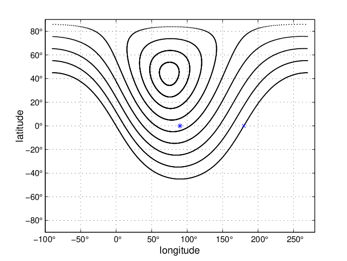
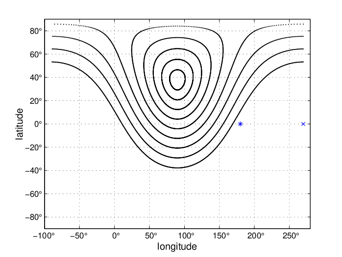
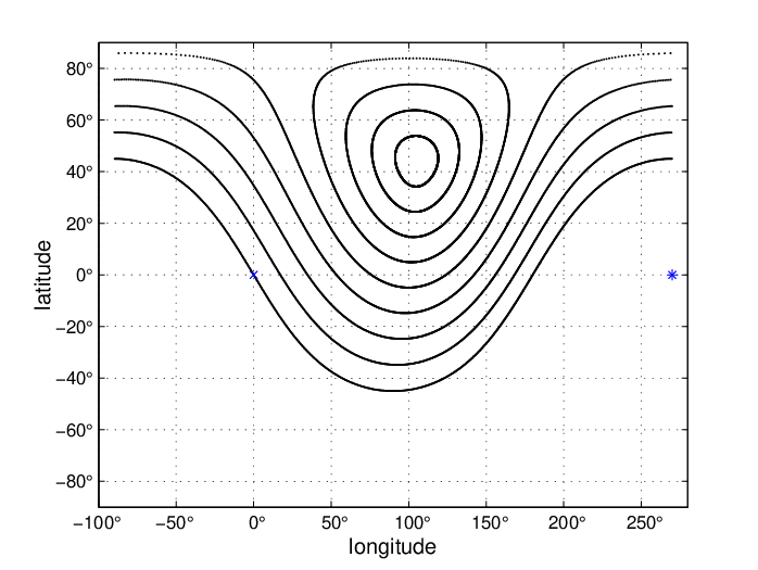
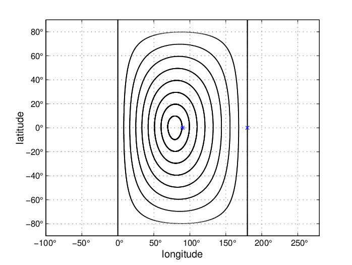
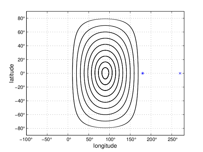
We can now plot closed curves of emission directions for specific choices of parameters. By showing curves for values of that differ by we can identify the area between two closed curves as the beam annulus for many choices of and .
Figures 7 and 8 show curves for . An observer fixed in position in the astronomical reference frame will measure the pulsar to be moving at speed , the speed that is used in our Lorentz transformation. Figure 7 shows results for , and Fig. 8 for . In each panel curves are given for 9 values of from (innermost) to (outermost), in increments; the area between any two curves in this sequence can be taken as the beam annulus. The 4 different panels in Fig. 7 and the 4 in Fig. 8 correspond to 4 different values of , the location of the SMBH in its motion around the pulsar (i.e., of the pulsar around the black hole). The value of in each panel is indicated by a small asterisk at zero latitude.
For the most part, the distorted shapes in Figs. 7 and 8 are the manifestations of geometry, the plotting of circles on a sphere in a cartesian coordinate system. The relativistic aspects of these figures, i.e., those due to motion and aberration, play two roles: (i) They are the reason that there are difference among the 4 panels in Figs. 7, and that there are differences among the 4 panels in Figs. 8. (ii) Aberration accounts for the small left-right asymmetry that is apparent in some of the panels. Both these effects are small, because aberration effects are of order , which is only around 0.19 for annuli shown in the figures.
IV A specific scenario
The deflection of a pulsar beam towards an Earth-based telescope requires an overlap. The keyhole in Sec. II describes the direction in which a photon must be emitted if it is to be deflected toward the Earth. The distorted annulus in Sec. III describes the set of direction in which the pulsar beam is deflected. For there to be an observable event, the keyhole direction must fall within the annulus.
Determining when the keyhole enters and exits the annulus is complicated because both the keyhole direction and the shape and location of the annulus change with time, i.e., change as the pulsar goes around the SMBH (or – in our coordinate systems – as the SMBH goes around the pulsar).
The formalism developed above makes no assumptions about the orbit of the pulsar (it need not even be closed), and no assumptions about the precession of the pulsar spin axis. The formalism can be applied to any orbit, and any time variability of pulsar spin etc. In this section, to illustrate the application of the formalism as clearly as possible, we choose the pulsar to have a circular orbit, at radius , and we ignore precession of the spin axis. As in previous sections we describe the motion as the SMBH going around the pulsar. For our example, in Fig. 9, we take , and take the pulsar beam to be confined between and . As pictured in Fig. 6 the SMBH is moving counter-clockwise, and we take it to be at (i.e., in the plane) at time . We choose to place the Earth observer at longitude and latitude . The Earth observer location is shown as a small blue asterisk in Fig. 9.
In Fig. 9, the thin red curve represents the trajectory of the keyhole. Because we have chosen to have the SMBH start at , the corresponding keyhole starts at around and is moving in the direction of increasing longitude . When the SMBH moves to the longitude marked by the magenta asterisk, at , the keyhole moves into the annulus; the thin red curve of keyhole location crosses the magenta curve which represents the boundary of the beam annulus at that moment. At this crossing event, pulses start to become detectable by the Earth observer. This period of observability (thickened segment of the keyhole trajectory) extends to the configuration at which the SMBH is at , denoted by the large blue asterisk, the SMBH position that corresponds to the trajectory of the keyhole (the thin red curve) passing the blue curve representing the boundary of the beam annulus at that moment of crossing. The number of pulses observable depends on the spin rate of the pulsar, but in any case will be large since the pulsar spin period is 8 or more orders of magnitude smaller than the orbital period.
After more than half an orbit passes, the SMBH is at (black asterisk) and the keyhole trajectory passes the black curve representing the boundary of the beam annulus. This starts a period of pulse observability which ends when the SMBH is at (green asterisk), corresponding to the keyhole trajectory passing the green curve that represents the boundary at that crossing.
It should be understood that the green and the magenta curves both represent the directions of photons emitted at , but they represent those directions for different locations of the SMBH relative to the pulsar. Similarly, the black and blue curves both represent the directions of photons emitted at .
In Fig. 10, we represent sequences of pulses for four epochs: black (corresponding to a time shortly after the passage of the keyhole trajectory crosses the black annulus curve), green, magenta and blue (similarly). The unit of time in each panel is the “proper” pulsar spin period, the spin period measured by an observer comoving with the pulsar. The value of that unit, in terms of , or of seconds, need not be specified. We assume only that the unit is many orders of magnitude less than the pulsar orbital period, so that many pulses are emitted with no substantial change in the pulsar-SMBH-Earth configuration. Without specifying a particular pulse period, we can compare the period of reception of pulses characteristic of each epoch.
The two upper panels show several pulses (vertical lines) from the epochs of the black and green keyhole-annulus crossings. The alignment of the pulses with the timing marks in Fig. 10 shows that the observed pulse period, in both cases, is slightly longer than the proper pulse period, although it is barely noticeable in the case for the black epoch). For both events the pulsar is moving almost transverse to the direction to the Earth. The photon path from the pulsar to the Earth is, therefore, only very slightly affected by the pulsar motion, and the effect on the received pulse period is negligible. The lower two panels correspond to the magenta and blue epochs. In both cases the pulsar is moving towards the Earth at pulse emission. For these epochs the photon path starts out generally away from the Earth, winds around the SMBH and proceeds towards the Earth. As the pulsar moves toward the Earth this backward then forward photon path increases in length thereby producing a redshift-like lengthening of the period between pulses. This pulse-period lengthening gives a noticeable difference between the observed and the proper pulse period.
The effects of attenuation, described by Eq. (1) are even more noticeable. For the upper panels showing the epochs of the black and the green events, the intensity is approximately 9% and 8% respectively of the intensity of a direct beam. For the lower panels showing the epochs of the magenta and blue events the attenuation is greater; the beam intensity is approximately 0.6% and 0.5% that of a direct beam. These attuations are not due to photon redshifts. For these epochs the pulsar is not receding from the Earth and, in any case, the red/blueshift effects are very small and are not included in Eq. (1), for reasons explained in Sec. II and in Paper I.

 |
 |
 |
 |
V Summary and Conclusions
We have set down the principles and the methods of calculation for analyzing the observational effects of a nonspinning black hole on a pulsar signals. In particular, we have shown that the calculation of pulse timing and intensity involves solving two problems simultaneously: that of the the beam annulus distorted by aberration, and that of the keyhole position and trajectory. Once these calculations are done, one can quickly infer the strong field effect on the pulse period and the beam attenuation for any epoch of motion.
The beam annulus computation starts with the pulsar’s beam details: the direction of its spin axis, and the orientation and width of its radio beam. Photon directions, most naturally specified in the frame of the pulsar, must then be transformed to the astronomical frame so that aberration effects are taken into account. The algorithm for doing this is set down in Sec. III.
For any pulsar-SMBH-Earth alignment, the keyhole direction is the photon emission direction (in the astronomical frame) for which a photon will be deflected towards the Earth. This direction must lie in the pulsar-SMBH-Earth plane, and the necessary deflection angle is determined by the pulsar-SMBH-Earth angles in that plane. The keyhole direction in that plane is inferred from the deflection angle by inverting the universal function developed in Paper I. The specific calculational steps are given in Eqs. (2)– (5). The relative simplicity of this method is the main motivation for ignoring the rotation of the SMBH.
Once the pulsar trajectory is specified, the two parts of the analysis are brought together. For any pulsar-SMBH-Earth alignment, it is determined whether the keyhole overlaps the beam annulus. Since the beam annulus shape, due to aberration effects, depends on the pulsar velocity, the shape must be calculated for each new position of the pulsar.
Though the use of the universal function greatly simplifies the calculations, the exploration of the parameter space for pulsars in Sgr A∗ is still inconveniently broad. This is particularly true because pulsar orbits near Srg A∗ may be highly eccentric, thereby adding to the already large set of parameters that constitute a model.
A minor but useful simplification is to ignore the aberration effects on the beam annulus, so that the beam annulus is fixed in the astronomical frame once and for all. (Precession of the pulsar spin axis is also ignored.) The aberration, in any case, is of order of the pulsar velocity divided by , and will be small. We have seen that the effects are small with the choice we have made, for the model in Secs. III and IV. Yet, even for orbits of high eccentricity, , a velocity is much more relativistic than what is likely to be the case for pulsars that are beaming past the SMBH.
A more detailed discussion of plausible astrophysical models will be given elsewhere [2]. Here we only point out that an epoch of observability will typically be of order of 10∘ or more of the pulsar orbit. This translates to millions of seconds for the most tightly bound pulsars in the Galactic center. Since pulsar spin periods are typically less than, or much less than a second, the pulse train for an epoch of observability will involve a large number of pulses. The timing and intensity patterns of that pulse train can reveal much about the strong field region through which the pulses traveled.
VI Acknowledgment
We gratefully acknowledge support by the National Science Foundation under grants AST0545837, PHY0554367, and 0734800. We also thank the NASA Center for Gravitational Wave Astronomy at University of Texas at Brownsville. YW acknowledges support by the Chinese National Science Foundation under grant 10773005.
References
- [1] Campana, S., Parodi, A., & Stella, L. 1995, MNRAS, 277, 1162
- [2] Creighton, T., Price, R. H., Wang, Y., & Jenet, F. A. 2009, in preparation
- [3] Freitag, M., Amaro-Seoane, P., & Kalogera, V. 2006, ApJ, 649, 91
- [4] Goicoechea, L. J., Mediavilla, E., Buitrago, J., & Atrio, F. 1992, MNRAS, 259, 281
- [5] Gorham, P. W. 1986, ApJ, 303, 601
- [6] Laguna, P., & Wolszczan, A. 1997, ApJ, 486, L27
- [7] Lazio, J., Deneva, J. S., Bower, G. C., Cordes, J. M., Hyman, S. D., Backer, D. C., Bhat, R., Chatterjee, S., Demorest, P., Ransom, S. M., & Vlemmings, W. 2006, Journal of Physics Conference Series, 54, 110
- [8] Melia, F. 2007, The Galactic Supermassive Black Hole (Princeton: Princeton University Press)
- [9] Muno, M. P., Baganoff, F. K., Brandt, W. N., Morris, M. R., & Starck, J.-L. 2008, ApJ, 673, 251
- [10] Oscoz, A., Goicoechea, L. J., Mediavilla, E., & Buitrago, J. 1997, MNRAS, 285, 413
- [11] Pfahl, E., & Loeb, A. 2004, ApJ, 615, 253
- [12] Wang, Y., Jenet, F. A., Creighton, T., & Price, R. H. 2009, ApJ, 697, 237, (Paper I)