Is there a Relationship between the Elongational Viscosity and the First Normal Stress Difference in Polymer Solutions?
Abstract
We investigate a variety of different polymer solutions in shear and elongational flow. The shear flow is created in the cone-plate-geometry of a commercial rheometer. We use capillary thinning of a filament that is formed by a polymer solution in the Capillary Breakup Extensional Rheometer (CaBER) as an elongational flow. We compare the relaxation time and the elongational viscosity measured in the CaBER with the first normal stress difference and the relaxation time that we measured in our rheometer. All of these four quantities depend on different fluid parameters - the viscosity of the polymer solution, the polymer concentration within the solution, and the molecular weight of the polymers - and on the shear rate (in the shear flow measurements). Nevertheless, we find that the first normal stress coefficient depends quadratically on the CaBER relaxation time. A simple model is presented that explains this relation.
Keywords:
elongational viscosity , normal stress , CaBER , polymer solutionsPACS
code , code1 Introduction
Viscoelasticity is probably the most prominent Non-Newtonian effect; it manifests itself a high elongational viscosity and a non zero first normal stress difference. Some examples of these effects are the filaments one can make with saliva or dye swell, i.e., a viscoelastic solution emerges from a pipe in the form of a jet with a width larger than the pipe’s width. Both of these effects are believed to be due to the same microscopic reason, the resistance to stretching of semi-flexible polymers. However, to our knowledge, there have been no experimental attempts to relate these two accessible quantities in a systematic manner.
The elongational viscosity of polymer solutions can be several orders of magnitude larger than the solvent viscosity, especially for flexible high molecular polymers. In contrast, the shear viscosity remains on the order of the solvent viscosity. Shear flow can be divided into a rotational part and an elongational part. The elongational part stretches the macromolecules and induces stress while the rotational part leads to a tumbling of the polymers, and the direction of stress gets averaged out. In pure elongational flow, the orientation of the stretching remains constant and the polymers get stretched more and more until, eventually, they are elongated to their contour length, and the elongational viscosity reaches a plateau. In many applications, elongational flow affects the processability more severely, e.g., in fiber spinning, spraying, deposition of pesticides, etc. where the flow is elongational, at least to a large extent.
However, the definition of the first Normal stress (with the components of the stress tensor) in shear flow compared to the definition of the elongational viscosity in elongational flow suggests the existence of a direct relation between these two quantities ( is the elongational rate). >From an experimental point of view, measurement of the elongational viscosity of dilute polymer solutions is a nontrivial task and only recently a method called CaBER (Capillary Breakup Extensional Rheometer) became available. A droplet is placed between two plates, and after they are separated by a linear motor the capillary bridge between them starts to shrink. Instead of break up, a cylindrical filament is formed due to the high viscoelastic stresses. By balancing surface tension and viscoelastic stresses an apparent elongational viscosity can be deduced by simply measuring the thickness versus time of the shrinking filament. In such a set-up, the elongational rate is chosen by the system and can not be controlled.
The relation between shear and elongational flows has been previously investigated. A principle approach was to determine the characteristic time constant of the filament in a CaBER setup that shrinks exponentially in time, and to compare it with the respective shear quantities (shear viscosity and relaxation time) using different models (typically, Zimm [1] or Rouse [2]). Gupta et al. [3] performed shear and oscillatory shear experiments, which they compared to extensional rheological data with a filament-stretching device [4, 5]. The samples were different polystyrene solutions. They found that the shear properties could be well described by the Zimm model, whereas the extensional data show a direct dependence of the stress growth on concentration and molecular weight of the polymers; this agrees with the Rouse model. Nevertheless, by using a FENE-P model with Zimm parameters they were not able to predict the results or to fit the extensional data.
In 2003, Lindner et al. [6] tried to compare the elastic properties in elongational and shear flow by using an opposed nozzle rheometer [7] and a classical rotational rheometer, respectively. They explicitly tried to fit their rheometric measurements with the FENE-P model, but, to some extent, they were only able to fit the normal stress data. The shear thinning effects in their set of highly elastic solutions were not covered by the FENE parameters obtained from the normal stress data. Still, they could calculate the elongational viscosity from the FENE parameters and compare them to the measured elongational viscosity by adjusting the finite extensibility parameter .
Plog et al. [8] used the technique of capillary thinning rheometry to characterize the dependence of the CaBER relaxation time on the molar mass distribution of the polymers in solution. They found good agreement between the molecular weight distribution obtained from the CaBER measurements and experiments on size-exclusion-chromatography, multi angle laser light scattering and differential refractometry, but they were not able to correlate the results with standard rheometric measurements.
In 2006, Clasen et al. [9] published their work concerning the question of the determination of the overlap concentration of polymer solutions in CaBER experiments. They compared CaBER and small amplitude oscillatory shear (SAOS) measurements on polystyrene solutions below the "classical" overlap concentration. For the shear measurements, they found that the relaxation times of their solutions agree very well with the Zimm relaxation times and show only a slight increase when approaching the overlap concentration. The CaBER measurements, however, revealed quite different behavior: at low concentrations the relaxation times are below the Zimm values, but they continuously increase with increasing concentration, so that, for concentrations near the overlap concentration, the values are much higher. Therefore, they concluded that there must be a so called critical polymer concentration in elongational measurements, which is orders of magnitudes smaller than the overlap concentration that is found in shear experiments. The result of an increase in the relaxation time with increasing concentration, even below the overlap concentration, in an elongation experiment was also observed by Tirtaatmadja et al. [10] and by Amarouchene et al. [11], who both investigated the droplet detachment of polyethyleneoxide in glycerol/water mixtures or pure water, respectively.
Here, we compare the first normal stress coefficient, which we determined from rheometer measurements, with the relaxation time, which we measure in CaBER experiments. Thereby, we can directly relate the first normal stress difference to the elongational viscosity in polymer solutions. We find that the first normal stress coefficient depends quadratically on the CaBER relaxation time.
2 Theoretical Background
Despite the numerous theoretical contributions to the field, a full quantitative modeling of viscoelastic properties of complex fluids remains a challenge nowadays. However, standard models have been proven to describe important features of polymeric solutions within some limits. Among them, Oldroyd-B is a minimal model giving rise to viscoelastic effects. It consists of considering two beads connected by a Hookean spring suspended in an incompressible Newtonian fluid. The linear spring force puts no limit on the extent to which the dumbbell can be stretched. The FENE-P model (finitely extensible non-linear elastic) corrects for this unphysical behavior. We compared our data to those two models.
2.1 Oldroyd-B model
Based on the microscopic picture of an elastic dumbbell, the Oldroyd-B model is probably the simplest linear viscoelastic model that includes finite first normal stress differences. The continuum mechanical constitutive equation for the local stresses can be calculated from the microscopic dumbbell model by using any distribution function of the polymer in solution, and averaging over the number of molecules per unit volume [12]:
| (1) |
where represents the time constant of the Hookean dumbbells, is the thermal energy and is the velocity gradient tensor. In principle, one can now calculate the temporal evolution of the stress tensor for any flow situation. In the following two subsections, the relevant results for shear and elongational flow are presented.
2.1.1 Shear flow
For the polymer contribution to the shear stress one finds
| (2) |
where is the shear rate, and the first normal stress difference is given by:
| (3) |
The first normal stress coefficient is defined as , this then leads to [12]:
| (4) |
2.1.2 Elongational flow
In uniaxial elongation flow the polymers are stretched the most efficiently. They uncoil in the flow and build up large elastic stresses, and the elongational viscosity of the liquid increases severely compared to the solvent viscosity. Assuming a cylindrical filament in the CaBER, for a polymer solution, the elongational viscosity is the ratio between the first normal stress difference and the elongation rate and an analysis of the Oldrd-B model yields [13, 14]
| (5) |
where and are the normal stresses in the stretching and the radial direction, is the elongation rate, the surface tension that drives the thinning process and the thickness of the filament when it is formed. Here, we see that the polymer relaxation time characterizes the exponential growth of the elongational viscosity and the normal stress coefficient amplitude, two quantities that are experimentally accessible. Given this, it should be possible to experimentally relate normal stress characteristics to elongational properties of flexible polymer solutions.
In some cases, a transition from exponential thinning behavior of the filament to a linear regime has been reported. This is often used to extract a plateau value for the elongational viscosity, but the regime is typically very small and the validity of this approach might be questionable. If, indeed, polymers are stretched to a maximum, the pinch off dynamic should be governed by self similar laws that reflect the full hydrodynamic dynamics[15].
2.2 FENE-P model
One model that is supposed to describe flexible polymers reasonably well and includes their finite extensibility is the FENE model [12]. Furthermore, it can describe, in some limits, the effect of shear thinning. In our case, the solution for a stationary shear flow gives the following expressions for the polymer part of the viscosity and the normal stresses, respectively [12]:
| (6) |
| (7) |
Here, the parameters and represent the finite extensibility and the molecular relaxation time of the polymers, respectively, and are left as independent fit parameters. Small values of result in a description of very stiff polymers, whereas, for the limit of infinite , the equations 6 and 7 approach the respective equations for an Oldroyd-B fluid. Therefore, the FENE-P model is able to describe the shear thinning of a given polymer solution only as long as remains small.
3 Experimental methods
3.1 Sample preparation
Two different polymers in glycerol-water mixtures were used (see Table 1): Polyacrylamide (PAAm) with a molecular weight of g/mol (Fluka) and Polyethyleneoxide (PEO) with g/mol (Aldrich).
PAAm and PEO are flexible polymers. The different solubilities of the polymers limited us to different concentration ranges (cf. Table 1). For the solutions with low polymer concentrations in low viscosity solvents, the normal stresses could not be reasonably well determined. For the high polymer concentrations in very viscous solvents, it was not always possible to perform CaBER measurements because the filament showed strong deviations from a simple exponential thinning process. Finally, some solutions with a high polymer concentration in a glycerol-rich solvent could not be prepared. The polymers did not dissolve and the solution remained turbid. Aside from these limitations, we prepared and characterized all polymers with concentrations from 75ppm to 9600ppm, doubling the concentration from one solution to the next, and in glycerol-water mixtures, starting with water up to 80% glycerol in steps of 20%.Estimations from intrinsic viscosity measurements and from data from the literature indicated that the overlap concentrations for all solutions were on the order of .
All solutions were prepared with the following protocol: the respective amounts of polymers were slowly poured in water first. After some minutes of swelling at rest, the polymer-water mixture was gently stirred for 24 hours. For the glycerol-water solutions, the respective amount of glycerol was added and the solution was stirred again for 24 hours. All solutions were measured within one day, in order to minimize degradation.
| polymer | solvent | concentration c [ppm] |
| PAAm (5-6Mio) | 40/60 glycerol/water | 600, 1200, 2400 |
| 60/40 glycerol/water | 300, 600, 1200, 2400 | |
| 80/20 glycerol/water | 150, 300, 600, 1200, 2400 | |
| PEO (4Mio) | water | 1200, 2400, 4800 |
| 20/80 glycerol/water | 1200, 2400, 4800 | |
| 40/60 glycerol/water | 150, 300, 600, 1200, 2400, 4800 | |
| 60/40 glycerol/water | 150, 300, 600, 1200, 2400 |
3.2 Experimental Setups
3.2.1 Capillary Breakup Extensional Rheometer
Our Capillary Breakup Extensional Rheometer consists of two circular stainless steel plates with a diameter of 2mm. A droplet of the polymer solution was put between the two plates. The upper plate was then moved away by a linear motor, which is controlled by software. After separation of the plates, there was a hemispherical fluid reservoir at each of the two plates. Between these reservoirs a cylindrical filament formed, which thinned exponentially in time. The diameter of the thinning filament was measured with a high-speed camera (XS-5, IDT) with a resolution of 1280500, at a frame rate of 2100Hz. The filament was imaged with a microscope objective (Nikon) with fourfold magnification and the diameter was determined from the digital shadowgraphs (fig. 1) with a threshold algorithm.
The elongation rate in a capillary thinning experiment is given by [12]:
| (8) |
where is the minimum diameter of the cylindrical filament. The filament thins exponentially with time according to:
| (9) |
where is the diameter at which the exponential thinning starts, and is a characteristic time constant of the polymer solution . From equation 9 and 8, it follows that the elongation rate is constant and given by
| (10) |
The thinning dynamics result from the surface tension that tends to thin the filament and elongational viscosity () that resists thinning:
| (11) |
Using equation 10, this leads to:
| (12) |
This means that the elongational viscosity increases exponentially within time with the characteristic time constant , in accordance with equation 5 that was deduced by an analysis of the Oldroyd-B model.
3.2.2 Rheometer
The shear flow measurements are performed in a commercial rheometer (Haake MARS) with cone-plate geometry. Here, we used a cone with an angle of 2∘; the cone and the plate are 60mm in diameter, and the probe volume is 2.0ml. The cell is tempered to 20∘C via a Haake PhoenixII with an accuracy of 0.01∘C.
Data points were taken at shear rates between 1 and 2000. The shear rate has been changed on a logarithmic scale between and 250, and in linear steps of 25 for higher shear rates. Please note that the typical elongational rates that have been observed in CaBER measurements were of the same order of magnitude.
4 Measurements and Results
4.1 Capillary Breakup Extensional Rheometer
Our CaBER measurements are carried out by putting a droplet of the liquid that we want to investigate on the lower, fixed plate, and bringing the upper, movable plate into contact with the droplet. Then, the upper plate is pulled upwards and, thus, there is a thinning liquid bridge between the two plates (see Figure 1).

During this capillary thinning there are two different regimes: In the first one, the filament thins exponentially with time (cf. Equation 9). Typically, one also observes a second regime that is reached after the exponential one when the polymers are fully stretched. In this regime, the sample fluid might be seen as a Newtonian fluid but with an increased elongational viscosity. The linear behavior is consistent with theoretical and experimental considerations on Newtonian liquids. However, there exists no consistent approach to describe these two regimes by use of the same material parameters. Here, we restrict ourselves to the first regime, where the relaxation time is extracted (cf. Equation 9).

4.2 Rheometer
The rheometric measurements have been carried out in a straight forward manner with the procedure mentioned in section 3.2.2. Inertial effects occurring at high shear rates are corrected for [21].
We could then deduce the polymer relaxation time from normal stress measurements using equation 4. Furthermore, the respective fits for the FENE-P model were performed according to equation 6 and equation 7.

Figure 3 shows two exemplary data sets for the first normal stress difference of the different types of polymers. The data sets are fitted with a quadratic power law (Oldroyd-B fluid).
Finally, we would like to discuss the FENE-P fits for the PEO solutions. An analysis of the normal stress data yielded relaxation times similar to those of the elastic dumbbell model, but with a relatively large parameter b within the FENE model (Figure 4), meaning a high flexibility.


Right: Shear thinning effect of 4800ppm PEO in water. Respective fits are done with the FENE-P model, and the parameters determined from normal stress measurements (straight line) as well as the FENE-P model and free parameters (dotted line).
However, the same set of parameters does not describe the shear thinning of the polymer part of the viscosity fit (Figure 4).
The same result holds if the fits for and are performed simultaneously. The fits nicely reproduce the normal stress data but fail to describe the viscosity. A fit for the viscosity data alone can be performed reasonably well, but the parameters are far from being realistic.
Actually, the typical approach to extract a timescale from data is, indeed, to combine equation 2 and 3, and to divide the normal stress coefficient by the polymeric part of the viscosity. In this way the number density drops out of the equation but the drawback is that due to the shear thinning of the polymeric part of the viscosity it yields to a shear rate dependent time constant, which is also called a shear thinning relaxation time. Even if the relaxation times that we extracted by this method were on the same order of magnitude as the ones that we determined by use of the microscopic quantities, the data was scattered much more strongly, mostly due to the difficulty in determining the polymeric part of the viscosity precisely. Furthermore, it is not clear which shear rate should have been chosen for comparisons with the CaBER measurements.
4.3 Comparison between CaBER and Rheometer

Figure 5 shows the measured normal stress coefficient as a function of the characteristic time of filament thinning from the CaBER experiment, and this is shown for the two types of polymer solutions (PEO and PAAm) and for the whole range of concentrations indicated in table 1. One can notice that increases quadratically as a function of . This indicates a quantitative correlation between normal stresses and elongational viscosity. This is what we expected as the microscopic origin of the two effects is the resistance against stretching of the flexible chains of polymers. At first, the quadratic dependence of on seems to fulfill equation 4. However, contrarily to what is expected from equation 4, the relation between the first normal stress coefficient and the CaBER relaxation time is found to NOT depend on polymer number density . To investigate the reasons for this discrepancy, we will determine in the following how , on the one hand, and , on the other hand, scale with polymer number density and with the solvent viscosity .
We would now like to deduce a functional dependence of the normal stress and elongational viscosity data. We will use the relaxation time from the CaBER measurements, and the relaxation time and the first normal stress coefficient from the shear experiments.
It is already known from the literature that strongly depends on both polymer concentration and solvent viscosity; increases with increasing concentration or increasing viscosity (cf. [9] or [10] for example). For , the situation is less obvious. The Oldroyd-B model predicts that the relaxation time depends on the solvent viscosity but not on the polymer concentration. This directly follows from the definition of the relaxation time as , where is a friction coefficient which linearly depends on the solvent viscosity and is the spring constant of the Hookean dumbbell [12]. Nevertheless, experimentally determined relaxation times can show different behaviors. Of course, it is important if the concentration is below or above the so called overlap concentration . The overlap concentration is the concentration at which two polymers in a solution interact with each other; this can lead to, e.g., entanglements that increase the relaxation time of the solution. Above this overlap concentration a solution is called semidilute, whereas below , it is a dilute one [22]. The effect of polymer interactions is not considered in the Oldroyd-B model. Still, within the limits of a continuum mechanical approach it is often possible to deduce a physical understanding of the physical origin of certain viscoelastic flow phenomena.
>From the first normal stress difference measurements we deduce the relaxation time from equation 4 for a range of concentrations and solvent viscosities. We can then determine scaling laws for in the form:
| (13) |
This corresponds to a scaling for in the form:
| (14) |


Lower images: First normal stress coefficient of PAAm and PEO as a function of the solvent viscosity. Power law fits are applied for different polymer concentrations.
Figure 6 shows the dependency of on the polymer number density and on the solvent viscosity and is well described by power laws. is found to increase with the polymer concentration with an exponent around , and with the solvent viscosity with an exponent around .
The averaged values for each polymer are given in table 2.
With the experimental values of the exponents of and we can deduce the scaling exponents for as follows:
| (15) |
The dependency of on the polymer concentration and on the solvent viscosity was already investigated by Amarouchene et al. [11], Clasen et al. [9], Tirtaatmadja et al. [10] and Rodd et al. [18]. Again, we look for scaling laws in the form:
| (16) |
Figure 7 shows that the relaxation time deduced for filament thinning is well described by power laws. We found that increases linearly with solvent viscosity and with an exponent of on the polymer number density. The averaged values of the exponents are tabulated in table 2. Even if we are mostly interested in scaling laws, we should mention that the absolute values of and might differ by more than one order of magnitude with, typically, and only at higher concentrations or even .
For PEO in glycerol/water mixtures, Clasen et al. [9] and Tirtaatmadja et al. [10] both found that the relaxation time measured in an elongation experiment varies with , whereas Amarouchene et al. [11] observed an exponent of about 0.82 for PEO in water with a droplet detachment experiment.


Lower images: CaBER relaxation time of PAAm and PEO as a function of the solvent viscosity. Power law fits are applied for different polymer concentrations.
A theoretical prediction for the dependence of the polymer relaxation time on the concentration for disentangled semidilute polymer solutions is given by Rubinstein and coworkers Ref.[22]. The exponent depends on the solvent quality and might vary from , a good solvent, to a solvent. In this sense, one could simply explain the differences of and by a change in solvent quality. Even if phase separation effects in elongational flow have been reported [15], this does not seem to be likely - in both experiments the solutions were the very same. Similarly, one could imagine the dynamic in the CaBER experiment is better described by a theory of entangled semidilute solutions due to a larger elongation of the polymers and a larger effective volume. But, in this case, the exponents should be well larger than [22], in contradiction to our observations. Clasen et al. [9] also compared their findings for with the theoretical predictions by Rubinstein. They interpret a strong dependence of , even in the dilute regime, by an effective overlap concentration that is much smaller in elongational flow than in shear flow. However, Amarouchene et al.[11] found a dependency of down to 10 ppm.
| PAAm(=5-6Mio) | PEO(=4Mio) | |
|---|---|---|
| 1,4700,038 | 1,5600,010 | |
| ( vs. ) | ||
| 1,6960,026 | 1,6700,080 | |
| ( vs. ) | ||
| 0,8200,039 | 0,8350,155 | |
| ( vs. ) | ||
| 0,9510,024 | 0,9820,082 | |
| ( vs. ) |
The CaBER relaxation time, as well as the normal stress relaxation time, of the different polymer solutions depends on the viscosity. Thus, for solvents with a similar exponent, these quantities can be rescaled to coalesce on one graph. The results for both polymer types are shown in figure 8 for the CaBER and in figure 9 for the normal stress relaxation times, respectively.

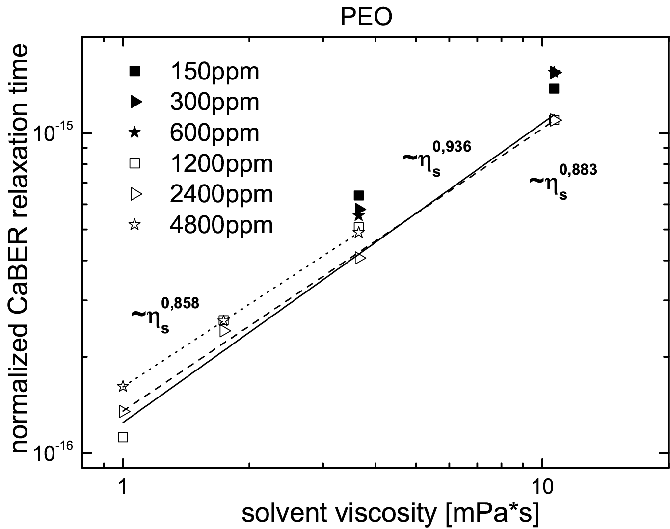


Here, one can clearly see that, for each polymer type, the rescaled CaBER and normal stress relaxation times as a function of the solvent viscosity fall on one curve. Apparently, the remaining dependency on the solvent viscosity shows almost the same exponent for the CaBER and the normal stress relaxation times, independent of the polymer type.
>From the and , we are now able to compare the two different relaxation times that were determined in the CaBER () and in the rheometer (), respectively. Dividing by , we get:
| (17) |
In another step, one of the two relaxation times can be rescaled by the number density per unit volume of the polymers in solution, to adapt the normal stress relaxation time to the CaBER one. Comparing the two dependencies of these timescales, one recognizes a difference of in their potential behavior. Scaling the normal stress relaxation time with a factor of , the relation between this quantity and the CaBER relaxation time becomes linear (see figure 10).

The dependencies on the solvent viscosity are the same for the CaBER and the normal stress relaxation time; this fact leads to the result that the viscosity cancels out if one compares the first normal stress coefficient with the CaBER relaxation time. Since the scaling between and is simply the square root of the number density per unit volume, the additional factor in equation 4 is canceled out too, meaning that we get a quadratic dependency if we plot versus (figure 5). It is worth mentioning that this plot can be performed without any additional scaling, i.e., the data that are determined from the data are directly plotted versus the that are measured in the CaBER.
5 Conclusion
In conclusion, we have shown that the normal stress coefficient shows a quadratic dependence on the relaxation time that we measured in the Capillary Breakup Extensional Rheometer. This can be motivated by simple assumptions, i.e., by the fact the polymer relaxation time that has been determined in in shear flow depends only weakly on concentration while for the CaBER relaxation time an almost linear dependence was found. This result could be obtained because it was found that for long-chained, flexible polymers (PAAm, PEO), one can quadratically fit the shear rate dependence of the first normal stress difference , as predicted by the Oldroyd-B model. From this fit, we obtained the first normal stress coefficient . The FENE-P showed no advantage to the simple Hookean elastic dumbbell model (Oldroyd-B).
The dependence of the respective relaxation times on solvent viscosity is roughly the same for CaBER and Rheometer data, i.e., it is close to a linear dependence. Furthermore, the dependency on the number of polymers for the two relaxation times differs by a factor of . Scaling one relaxation time with this factor, one gets a linear relationship to the other one. This scaling exactly explains the direct quadratic dependence of the first normal stress coefficient on the CaBER relaxation time. The additional linear factor in equation 4 is balanced by the dependence of on . In summary, we showed that there exists a very prominent and direct relationship between the elastic fluid properties in a stationary shear experiment and the parameters determined in a non-stationary extensional flow.
References
- [1] B. Zimm, Dynamics of polymer molecules in dilute solution: viscoelasticity, flow birefringence and dielectric loss, J. Chem. Phys. 24 (1956) 269.
- [2] P. Rouse Jr., A theory of the linear viscoelastic properties of dilute solutions of coiling polymers, J. Chem. Phys. 21 (1953) 1272.
- [3] R. Gupta, D. Nguyen, T. Sridhar, Extensional viscosity of dilute polystyrene solutions: Effect of concentration and molecular weight, Phys. Fluids 12 (2000) 1296.
- [4] T. Sridhar, V. Tirtaatmadja, D. Nguyen, R. Gupta, Measurement of extensional viscosity of polymer solutions, J. Non-Newtonian Fluid Mech. 40 (3) (1991) 271–280.
- [5] V. Tirtaatmadja, T. Sridhar, A filament stretching device for measurement of extensional viscosity, J. Rheol. 37 (1993) 1081.
- [6] A. Lindner, J. Vermant, D. Bonn, How to obtain the elongational viscosity of dilute polymer solutions?, Physica A: Statistical Mechanics and its Applications 319 (2003) 125–133.
- [7] G. Fuller, C. Cathey, B. Hubbard, B. Zebrowski, Extensional viscosity measurements for low-viscosity fluids, J. Rheol. 31 (1987) 235.
- [8] J. Plog, W. Kulicke, C. Clasen, Influence of the molar mass distribution on the elongational behaviour of polymer solutions in capillary breakup, Appl. Rheol. 15 (1) (2005) 28–37.
- [9] C. Clasen, J. Plog, W. Kulicke, M. Owens, C. Macosko, L. Scriven, M. Verani, G. McKinley, How dilute are dilute solutions in extensional flows?, J. Rheol. 50 (2006) 849.
- [10] V. Tirtaatmadja, G. McKinley, J. Cooper-White, Drop formation and breakup of low viscosity elastic fluids: Effects of molecular weight and concentration, Phys. Fluids 18 (2006) 043101.
- [11] Y. Amarouchene, D. Bonn, J. Meunier, H. Kellay, Inhibition of the finite-time singularity during droplet fission of a polymeric fluid, Phys. Rev. Lett. 86 (16) (2001) 3558–3561.
- [12] R. Bird, R. Armstrong, O. Hassager, Dynamics of polymeric liquids, Vol. 1, Fluid mechanics, John Wiley& Sons, New York, 1987.
- [13] P. Schümmer, K. Tebel, A new elongational rheometer for polymer solutions, J. Non-Newtonian Fluid Mech. 12 (3) (1983) 331–347.
- [14] C. Clasen, J. Eggers, M. Fontelos, J. Li, G. McKinley, The beads-on-string structure of viscoelastic threads, J. Fluid Mech. 556 (2006) 283–308.
- [15] R. Sattler, C. Wagner, J. Eggers, Blistering pattern and formation of nanofibers in capillary thinning of polymer solutions, Phys. Rev. Lett. 100 (16) (2008) 164502.
- [16] M. Renardy, Some comments on the surface-tension driven break-up(or the lack of it) of viscoelastic jets, J. Non-Newtonian Fluid Mech. 51 (1) (1994) 97–107.
- [17] M. Renardy, A numerical study of the asymptotic evolution and breakup of Newtonian and viscoelastic jets, J. Non-Newtonian Fluid Mech. 59 (2-3) (1995) 267–282.
- [18] L. Rodd, T. Scott, J. Cooper-White, G. McKinley, Capillary break-up rheometry of low-viscosity elastic fluids, Appl. Rheol. 15 (1) (2005) 12–27.
- [19] M. Oliveira, G. McKinley, Iterated stretching and multiple beads-on-a-string phenomena in dilute solutions of highly extensible flexible polymers, Phys. Fluids 17 (2005) 071704.
- [20] M. Oliveira, R. Yeh, G. McKinley, Iterated stretching, extensional rheology and formation of beads-on-a-string structures in polymer solutions, J. Non-Newtonian Fluid Mech. 137 (1-3) (2006) 137–148.
- [21] C. Macosko, Rheology: principles, measurements, and applications, VCH: Wiley-VCH, New York, NY, 1994.
- [22] M. Rubinstein, R. Colby, Polymer physics, Oxford University Press, USA, 2003.