ISW measurements with photometric redshift surveys: 2MASS results and future prospectsThanks: Scottish Universities Physics Alliance
Abstract
In a flat universe dominated by dark energy, the Integrated Sachs-Wolfe (ISW) effect can be detected as a large-angle cross-correlation between the CMB and a tracer of large scale structure. We investigate whether the inconclusive ISW signal derived from 2MASS galaxy maps can be improved upon by including photometric redshifts for the 2MASS galaxies. These redshifts are derived by matching the 2MASS data with optical catalogues generated from SuperCOSMOS scans of major photographic sky surveys. We find no significant ISW signal in this analysis; an ISW effect of the form expected in a CDM universe is only weakly preferred over no correlation, with a likelihood ratio of 1.5:1. We consider ISW detection prospects for future large scale structure surveys with fainter magnitude limits and greater survey depth; even with the best possible data, the ISW cross-correlation signal would be expected to evade detection in of cases.
Keywords:
1 Introduction
It is now widely accepted that the universe today is dominated by Dark Energy. Evidence for this comes from a number of sources: supernovae observations indicate a luminosity distance-redshift relation consistent with accelerated expansion (Riess et al., 1998; Perlmutter et al., 1999); the combination of CMB and galaxy clustering measurements places tight constraints on the Dark Energy density (Efstathiou et al., 1990; Efstathiou et al., 2002; Spergel et al., 2007) and Baryon Acoustic Oscillation (BAO) measurements suggest an angular diameter distance-redshift relation consistent with Dark Energy (Eisenstein et al., 2005; Percival et al., 2007).
Further independent evidence for Dark Energy can be provided by detection of the Integrated Sachs-Wolfe (ISW) effect, a gravitational secondary anisotropy in the CMB. The ISW effect is a net change in the energy of a CMB photon as it passes through evolving gravitational potential wells. The ISW temperature fluctuations introduced via the ISW effect can be calculated from
| (1) |
where and denote the times today and at last scattering respectively; is the position along the line of sight of the photon at time and is the gravitational potential (Martinez-Gonzalez et al., 1990).
The ISW effect is a large scale phenomenon: temperature fluctuations tend to cancel on smaller scales as photons pass through many potential wells (Hu & Dodelson, 2002). The ISW effect is sub-dominant to the primary CMB anisotropies and exists on scales where cosmic variance is large, making its detection from CMB data alone infeasible. Instead, the cross-correlation between CMB maps and tracers of large scale structure is used (Crittenden & Turok, 1996). Many different tracers have been correlated e.g. X-ray (Boughn & Crittenden, 2005); Sloan Digital Sky Survey (Fosalba et al., 2003; Scranton et al., 2003); Luminous Red Galaxies (Granett et al., 2009; Sawangwit et al., 2010); radio (Nolta et al., 2004; Pietrobon et al., 2006); and quasars (Giannantonio et al., 2006). Not all of these lead to significant signals, but the strongest claimed detections currently lie at the level. Giannantonio et al. (2008) cross-correlated data from a number of different large scale structure surveys with WMAP CMB data and reported an overall ISW effect that was significant at the level.
Afshordi et al. (2004) cross-correlated the Two Micron All Sky Survey (2MASS, Jarrett, 2004) and year-1 WMAP data (Bennett et al., 2003) and claimed to detect the ISW effect at . However, no significant effect was found in the updated work of Rassat et al. (2007) (hereafter R07), who correlated 2MASS with the year-3 WMAP CMB data (Hinshaw et al., 2007). In the present paper, we investigate whether the addition of photometric redshifts to the 2MASS survey data can boost the significance of any ISW signal. We also consider detection prospects for similar surveys with fainter magnitude limits and surveys with greater depth.
For ease of comparison with R07 we adopt the same cosmological model, namely a flat universe with , where the Hubble parameter is 100 kms-1Mpc-1, spectral index , and . Section 2 describes the data that we use in this paper and details of the masks for the galaxy and CMB maps. Section 3 outlines the theoretical cross-correlation signal expected in a CDM universe and Section 4 presents the results of our harmonic space cross-correlation analysis. Section 5 assesses the statistical power of the method used here as a detection tool, and investigates the detection prospects of more ambitious large scale structure surveys. Our conclusions are presented in Section 6.
2 Data
The large scale structure dataset used in the cross-correlation analysis is by far the greatest source of uncertainty. On the scales of the ISW effect, the CMB data are signal dominated (Spergel et al., 2007) whilst the galaxy data are afflicted by shot noise, uncertainties in the bias relation and photometric redshift errors.
2.1 2MASS galaxy data
2MASS is an all-sky survey in the J, H and K bands. The final extended source catalogue (XSC) contains over 1.6 million objects, over 98% of which are galaxies (Jarrett, 2004). This dataset is ideal for constructing maps of galaxy mass density since near infrared selection means that 2MASS is sensitive to old stars and hence the most massive structures.
Photometric redshifts for the 2MASS XSC have been generated by matching the 2MASS data with optical catalogues generated from SuperCOSMOS scans of the major photographic sky surveys (UKST in the south; POSS2 in the north). Details of the SuperCOSMOS catalogue construction process are given in Hambly et al. (2001). These catalogues have been given an accurate photometric calibration using a mixture of SDSS photometry, plate overlaps, and requiring uniformity in average colour between optical band and 2MASS ; the details of the process are described in Peacock et al. (2010). The photographic data define an all-sky optical galaxy catalogue in photographic ,, bands, reaching completeness limits of approximately , , . Since the -band plates are significantly less deep, they were not used in the current analysis, leaving a 5-band dataset from which photometric redshifts were to be derived. Owing largely to SDSS, 2dFGRS, and 6dFGS, a very substantial set of calibrating spectroscopy exists – for about 30% of the catalogue. It was therefore possible to take a highly direct approach to the generation of photometric redshifts, averaging over neighbours of known redshift at a given location in the 5-band magnitude space. By using magnitudes rather than colours, this automatically builds in information from the luminosity function, so that bright galaxies are never allocated an extreme redshift that would require them to have an unrealistic luminosity. As a result, the scatter in photometric redshift declines towards , as shown in Fig. 1. The overall rms in is 0.033. By construction, this process yields photometric redshifts that are unbiased in that the mean true redshift at given is equal to . An inevitable consequence is that there is then a bias in at given true : is overestimated near and underestimated at high , by an offset of 0.02 to 0.03. In any case, what we will need below is the ability to predict the distribution of true from a band of ; provided this is known, any bias is unimportant.
The optical filter properties in UKST and POSS2 are very slightly different, so the process was performed separately in the two hemispheres. However, there is deeper calibrating spectroscopy in the north, which introduces the possibility of a small bias. We therefore made a small rescaling as a function of redshift so that the global redshift distributions in each hemisphere were forced to be identical (in shape, but not in number) for our standard extinction-corrected -selected galaxy sample.

We construct 3 galaxy subsamples in approximately independent photometric redshift slices of thickness out to . The true redshift distribution of galaxies in each of these slices is calculated using the calibrating spectroscopic information; these are shown in Fig. 2. We parametrize the redshift distributions using
| (2) |
and perform a least squares fit to obtain the distribution parameters. The best-fitting values of , and for each photometric redshift slice are given in Table 1. It is clear that the slice makes very little contribution to the 2MASS sky distribution; yet by virtue of its larger volume, this slice will double the total ISW signal compared to a limit at . We may thus hope that the use of redshift information in the current study will improve the chances of detection.

| Slice | |||||
|---|---|---|---|---|---|
| 451329 | 195789 | 0.88 | 2.24 | 0.076 | |
| 258673 | 101912 | 3.46 | 2.27 | 0.104 | |
| 19162 | 8543 | 17.4 | 2.12 | 0.083 |
It is necessary to mask the region of sky around the Galactic plane before making the galaxy overdensity maps, since the survey is incomplete here and confusion is more likely. Following R07, we use the dust maps of Schlegel et al. (1998) to mask regions with -band reddening , which leaves approximately 67% of the sky unmasked. For the cross-correlation analysis we impose magnitude cuts on the extinction corrected 2MASS data to ensure uniform coverage across the whole sky. The number of galaxies remaining in each of the photometric redshift slices is also given in Table 1.
We use HEALPix software (Górski et al. 2005; see also http://healpix.jpl.nasa.gov) to generate maps of the galaxy overdensity and to compute the spherical harmonic coefficients used in the cross-correlation analysis. Fig. 3 shows the galaxy overdensity in each of our photometric redshift slices.


2.2 WMAP CMB data
We take our CMB temperature data from the third year WMAP results (Hinshaw et al., 2007). Cross-correlations are computed for the 3 bands least contaminated by Galactic foregrounds (, and ) and also for the Internal Linear Combination (ILC) map. To minimise the effects of Galactic foregrounds we use the foreground reduced sky maps in which models for synchrotron, free-free and dust emission have been subtracted. It is however prudent to mask the WMAP maps at low Galactic latitudes and the WMAP Kp2 mask is used to this end, leaving of the sky unmasked.
The fact that both the galaxy maps and the CMB maps are masked will mean that spherical harmonic coefficients measured from the maps are not exact and an estimator needs to be used. Here, following R07, we compensate for the lack of sky coverage using the factor in equation (15).
We now summarise the necessary theory of the ISW effect (see e.g. Cooray et al. 2002, Afshordi et al. 2004 for details).
3 Theory and galaxy bias
Expanding the projected galaxy density field in a given redshift shell and the ISW temperature fluctuations in spherical harmonics, the cross correlation between the galaxy overdensity field and the CMB temperature field is:
| (3) |
where and are the spherical harmonic coefficients for the galaxy overdensity and temperature fields respectively and is the Kronecker delta.
In Fourier space and within the linear regime, Poisson’s equation relates the time derivative of the potential field to the matter density field:
| (4) |
where is the linear growth factor, normalised to today. From the definition of the ISW temperature fluctuations we then have:
| (5) | |||||
where denotes the matter overdensity field today, and are unit vectors and the exponential has been re-expressed in terms of spherical Bessel functions and spherical harmonics .
Within each redshift slice we calculate the projected galaxy overdensity , which is related to the three-dimensional galaxy overdensity via
| (6) |
where is the background galaxy number density and is comoving distance; thus is the effective radial weight applied to the density field.
Assuming a linear bias relation to relate galaxy and matter overdensities , the galaxy expansion coefficients are:
| (7) |
where once again the matter overdensity is evaluated today and is a unit vector.
Now the cross correlation can be written as
| (8) | |||||
where .
Limber’s approximation can be used to eliminate the spherical Bessel functions by using the small angle limit
| (9) |
Applying this to equation (8) gives:
| (10) | |||||
Fig. 4 shows the expected cross-correlation for each of our galaxy redshift shells. The peak of the cross correlation can be seen to shift to higher multipoles at higher redshifts as the power spectrum peak shifts to higher multipoles (a given physical scale will subtend a smaller angle when viewed from further away, i.e. will correspond to a higher multipole). The Limber approximation is valid here for .

Following an identical method, the galaxy auto-correlation is given by
| (11) |
or on applying the Limber approximation (Kaiser, 1992),
| (12) |
3.1 Galaxy bias
The galaxy bias is expected to change with : the furthest redshift shell is populated only by the brightest, most massive galaxies, which are known to be more strongly clustered (Park et al., 1994; Loveday et al., 1995). In order to determine the bias in each redshift slice, we use the galaxy angular power spectra. The form of the angular power spectrum in each slice can be predicted given a three-dimensional power spectrum using equations (11) and (12). The effective bias of the predicted spectrum can then be adjusted to match observations. In linear theory, bias cannot be determined independently of which also acts to renormalize the power spectrum, . In what follows, we therefore fix the value of at 0.75 and fit only for .
We use CAMB (Lewis et al., 2000) to generate non-linear matter power spectra for our cosmological model (see Section 1) and output the three-dimensional spectra at redshifts at the mid-point of each redshift shell in question. Although only strictly valid in linear theory, we evolve the non-linear power spectrum for each slice according to the growth function; this is thought to be a good approximation to the non-linear power spectrum on the linear and quasi-linear scales where we will fit for the bias. We have two sources of data that can be used to measure the angular power in each redshift slice: the photometric redshift data and the subset of this in the SDSS region where complete spectroscopic redshifts exist. Since the spectroscopic data exist only in a subregion, the angular power measured in this case will not be accurate on large scales. However, we should expect reasonable agreement between the photometric angular power and the spectroscopic angular power on smaller scales, up to differences due to sample variance and mask. Fig. 5 shows the shot noise corrected photometric and spectroscopic angular power spectra binned for in bins of width and the best-fitting predicted spectra for each of the redshift slices.


The fit is made using a maximum likelihood approach where the error bars are due to cosmic variance alone and are calculated from the model power spectra. The likelihood is
| (13) |
assuming the covariance matrix to be diagonal and therefore neglecting correlations between multipole bins (Blake et al., 2007). The vector is of differences between model and data, in each bin, and the diagonal elements of are
| (14) |
The fit is performed firstly for the photometric redshift data alone and secondly for the spectroscopic data alone. The best-fitting values for the bias are given in Table 2. Both the spectroscopic and photometric data show an increase in bias with redshift, which gives us confidence that this effect is real. The difference in bias between all photometric redshifts and SDSS true- information is small in comparison with this trend; given the restricted overlap of these samples and the correlated errors shown in Fig. 5, we believe that it is insignificant within cosmic variance.
| photo- only | 1.22 | 1.65 | 2.86 |
|---|---|---|---|
| SDSS only | 1.03 | 1.90 | 2.22 |
4 Cross-Correlation Analysis
In this work, we have two hypotheses: a null hypothesis , and a hypothesis where the cross-correlation is as expected in a CDM universe and is described by equations (8) and (10). We assume that the cosmological model is given; there are thus no adjustable parameters to consider, and the hypotheses can be compared by means of a simple likelihood ratio.
The cross-correlation for a pair of galaxy and temperature maps is calculated using
| (15) |
where the factors attempt to compensate for the loss of sky coverage due to the masks. In detail, masking also introduces correlations between multipoles, which we take into account by using a full covariance matrix to calculate the statistic; see Section 4.1. The cross-correlation data are binned to improve the signal-to-noise; we use 5 logarithmically spaced bins for and ignore for consistency with R07. From our 3 redshift slices with 5 multipole bins per slice, we have 15 data points in total to analyse for each WMAP band.
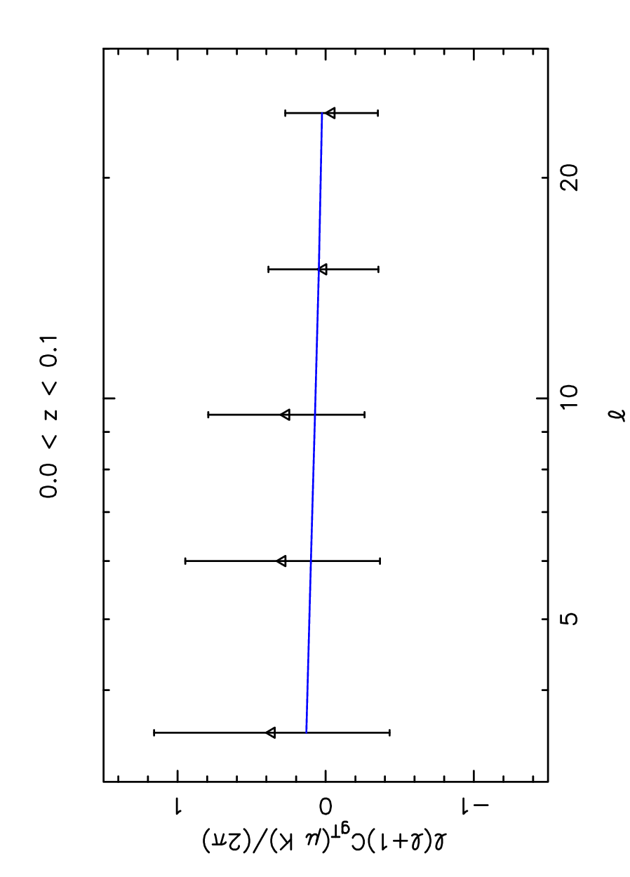
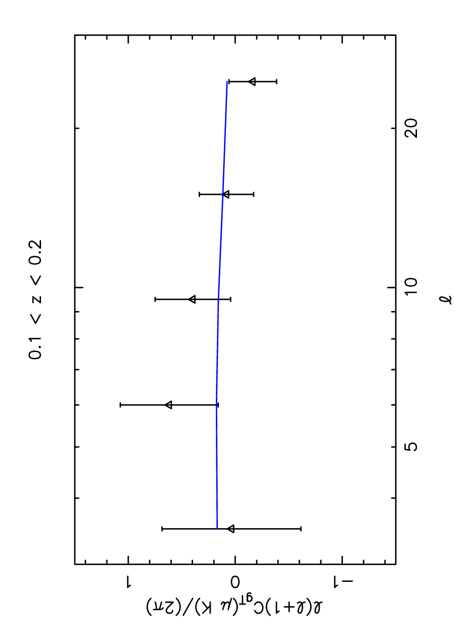
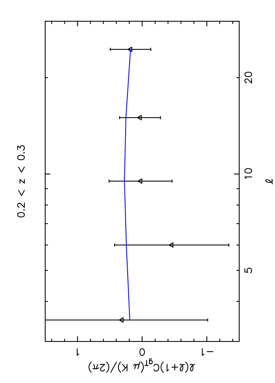
The cross-correlations measured in each redshift slice for each of the WMAP bands are shown in Fig. 6. The results are the same for each of the WMAP temperature maps considered, which is certainly consistent with the achromatic nature of the ISW effect. However, the plots also show the rms dispersion in under the null hypothesis of no ISW effect, from which it is clear that no signal is significantly detected. We quantify this by evaluating the statistic for each hypothesis using
| (16) |
where is the covariance matrix computed from simulations (see Section 4.1). The are the values of where is either zero or given by equations (8) and (10) for the fiducial hypothesis; are the measured cross-correlation values and labels the binned measurements.


The likelihood of each hypothesis is determined using
| (17) |
with the data vector whose components are defined above and the covariance matrix. In practice, the covariance matrix used in each case is calculated from simulations of the null hypothesis; this is a reasonable approximation given the subdominant nature of the ISW effect. Then
| (18) |
where and are the likelihoods for the two hypotheses.
4.1 Covariance matrix estimation
In order to calculate the covariance matrix for the values, we use 500 simulations each of independent CMB and galaxy density fields. The power spectrum used for the CMB Gaussian realizations is the best-fitting theoretical angular power spectrum found by the WMAP team (Spergel et al., 2007).
We generate simulations of the galaxy density fields by assuming a lognormal form for the measured 2MASS density field (Coles & Jones, 1991). This allows a rapid generation of realistic density fields, from which mock galaxies are drawn via Poisson sampling. We now have a set of simulated CMB and 2MASS galaxy maps with the same shot noise properties as the data.
The covariance matrix for the null hypothesis is estimated from the simulated data
| (19) |
where the data vector is defined as in equation (16). Using only simulations of the CMB correlated with the observed galaxy maps leads to an underestimation of error bars at the level on all scales, in agreement with Cabré et al. (2007). The error bars calculated from the diagonal elements of the covariance matrix are plotted in Fig. 7, and contrasted with the ISW signal expected in our default CDM universe.
4.2 Hypothesis testing
The values for each hypothesis are given in Tables 3, 4 and 5 considering bias values computed from photometric data only, SDSS data only and for consistent with R07 respectively. Each table has data for each redshift slice and for an analysis of all three slices together. The results depend to some extent on the values adopted for the bias in each slice. This does not affect the covariance matrix: values for the bias only affect the final results through an alteration of the expected signal.
| WMAP Band | ||||||||||||||
|---|---|---|---|---|---|---|---|---|---|---|---|---|---|---|
| ILC | 0.70 | 0.41 | 3.8 | 2.6 | 0.52 | 1.3 | 5.0 | 4.3 | 0.7 | |||||
| 0.68 | 0.32 | 3.7 | 2.5 | 0.68 | 1.2 | 5.1 | 3.9 | 1.2 | ||||||
| 0.63 | 0.33 | 3.9 | 2.8 | 0.65 | 1.4 | 5.2 | 4.4 | 0.8 | ||||||
| 0.63 | 0.33 | 3.6 | 2.6 | 0.67 | 1.3 | 4.9 | 4.3 | 0.6 | ||||||
| WMAP Band | ||||||||||||||
|---|---|---|---|---|---|---|---|---|---|---|---|---|---|---|
| ILC | 0.70 | 0.44 | 3.8 | 2.6 | 0.52 | 0.86 | 5.0 | 3.9 | 1.1 | |||||
| 0.68 | 0.36 | 3.7 | 2.4 | 0.68 | 0.82 | 5.1 | 3.5 | 1.6 | ||||||
| 0.63 | 0.37 | 3.9 | 2.7 | 0.65 | 0.96 | 5.2 | 4.0 | 1.2 | ||||||
| 0.63 | 0.37 | 3.6 | 2.6 | 0.67 | 0.96 | 4.9 | 3.9 | 1.0 | ||||||
| WMAP Band | ||||||||||||||
|---|---|---|---|---|---|---|---|---|---|---|---|---|---|---|
| ILC | 0.70 | 0.38 | 3.8 | 2.7 | 0.52 | 0.55 | 5.0 | 3.6 | 1.4 | |||||
| 0.68 | 0.28 | 3.7 | 2.6 | 0.68 | 0.58 | 5.1 | 3.4 | 1.7 | ||||||
| 0.63 | 0.30 | 3.9 | 2.8 | 0.65 | 0.66 | 5.2 | 3.6 | 1.6 | ||||||
| 0.63 | 0.30 | 3.6 | 2.7 | 0.67 | 0.67 | 4.9 | 3.8 | 1.1 | ||||||
In general, the results are low for the number of degrees of freedom; this was also noted by R07. We would expect values around for the individual redshift slices and for all slices together, but only the second redshift slice gives values that fall within these expected ranges. An analytic estimation of the error bars (Afshordi et al., 2004),
| (20) |
suggests errors that are even larger than those used here except for the lowest bin in the third redshift slice, so over-estimation of our error bars seems unlikely.
For the total analysis using the biases calculated from the photometric data alone, , which translates to a likelihood ratio of
| (21) |
This is a long way from decisive evidence for the ISW effect. Using the other bias values we prefer the fiducial hypothesis at levels of and for the SDSS bias and respectively. This latter scenario () is used by R07 and we find values very similar to their results in this case: against their . The differences between the analyses are our use of photometric redshifts, our slightly different magnitude cut of rather than and our use of simulations of the galaxy data as well as the CMB data to compute errors. As a result of simulating both CMB and galaxy data, we would expect our values to be smaller, as indeed is the case. Thus the main result of this paper is that photometric redshift information does not increase the sensitivity of the 2MASS data to the ISW effect.
5 Statistical power of current and future ISW experiments
Given the lack of a significant ISW detection from 2MASS, one is led to ask whether this is as expected, or whether we have been unlucky. We can address this by using our simulation apparatus to generate the distribution of values we could expect if the no-ISW null hypothesis were true
| (22) |
Here, the statistic itself is computed from the data in comparison with both the null hypothesis, and the alternative hypothesis but for data generated where is true. This distribution therefore shows how frequently a given threshold in would reject the null hypothesis when it is in fact true (the probability of making a Type I error).
In a similar manner, we can obtain a distribution of values under the assumption that the alternative hypothesis (CDM) is true. For each pair of simulated CMB and galaxy maps, we add to the CMB map the expected ISW effect for the galaxy map in question. The expected ISW signal can be computed by using equation (1) together with Poisson’s equation to find:
| (23) | |||||
where is the projected galaxy density field in the redshift shell under consideration and , where is the redshift at the midpoint of the shell.
The set of simulated galaxy and CMB+ISW maps allows us to calculate the distribution of the values we should expect if the alternative hypothesis were true:
| (24) |
We can thus measure the probability of making a Type II error (accepting the null hypothesis when the alternative is true) for a given threshold. Fig. 8 shows the two histograms computed from simulations of the CMB and 2MASS galaxy data for the different redshift slices used in the analysis.


A powerful statistical test would show a clear offset between the histograms in Fig. 8. In reality, we see very little offset between the distributions for this experiment. The final panel of Fig. 8 reveals that if the CDM hypothesis is true, a very large value of would be needed to rule out the null hypothesis with any confidence. There is an chance of obtaining a value greater than if the CDM hypothesis is true, and a chance of making a Type I error with this threshold.
If we were to adopt Jeffreys’ criterion (Jeffreys, 1948) that constitutes strong evidence for rejecting the null hypothesis, then such a threshold carries a chance of making a Type I error.
To make a decisive detection of the ISW effect we need distributions with a clearer offset and less overlap. The poor 2MASS results prompt us to ask how good the data would have to be to make a significant ISW detection. As the CMB data on these scales are already signal-dominated, any improvement must come from the galaxy data.
The power of a statistical test is defined as
| (25) |
where is the probability of making a Type II error with a threshold . A statistical test can be made arbitrarily powerful by altering the threshold, but a gain in power is offset by an increase in the probability of making a Type I error. We therefore define the ‘Optimal Power’ of a test as the power of that test with threshold chosen such that the probabilities of making Type I and Type II errors are equal. A larger Optimal Power indicates a ‘better’ statistical test in the sense that it is less likely to return the wrong conclusion from the data. The Optimal Power of this experiment is .
5.1 Same survey, fainter magnitude limit
Consider a survey with the same parameters as above but more galaxies at higher redshift (), equivalent to having a fainter magnitude limit for the survey. Following the same procedure used in Section 4.1, we simulate lognormal galaxy maps for this survey with bias and number density equal to the measured values for .
The CDM distribution in the third redshift slice (histograms not shown here) is narrower than that for the 2MASS experiment, although the ‘null’ distribution is largely unchanged, reflecting a reduction in shot noise which improves the ISW signal estimation. Looking at the analysis of the entire dataset together, the peak of the CDM distribution is shifted to a higher value and the distribution is narrower, leading to an increase in the offset between the peaks of the distributions. However, the Optimal Power for this experiment is , showing little improvement.
5.2 Deeper survey (more redshift slices)
We also investigate hypothetical deeper surveys, with characteristic redshift . The redshift distribution is computed using
| (26) |
where is constant and calculated from 2MASS galaxies with . We also consider varying . Generally, we shall show results for a maximum redshift up to 0.7.
We consider shells of width and take the true redshift distribution of galaxies in each slice as a Gaussian of width centred at the midpoint of the slice for ; the true redshift distributions calculated for the 2MASS data are used for . The galaxy bias in each slice is estimated using the simple assumption that bias is determined solely by the ratio of observed to expected numbers of galaxies in that slice, where the expected number of galaxies is found using . This means that bias is not intrinsically redshift dependent – the reason we see higher bias at higher redshift is because only the brightest, most massive galaxies are observed there. This seems a reasonable model for the redshifts we consider given the results of Magliocchetti et al. (2000), who see little evolution in bias over this range. In keeping with these assumptions, we use the bias in the three 2MASS redshift slices, together with the fraction of galaxies observed here, to deduce a relationship between these quantities. Our best-fitting relationship is
| (27) |
where is the fraction of galaxies observed.
Fig. 9 shows the histograms for this experiment with . The distributions for redshift slices with all show an offset and the null hypothesis distributions for these slices are slightly skewed towards negative values. The analysis of the full dataset for shows a clear offset between the peaks of the two distributions and considerable improvement in detection prospects.


Values of would be expected to occur (if the alternative hypothesis were true) around of the time and would lead to a fairly conclusive rejection of the null hypothesis ( chance of a Type I error). The Jeffreys criterion of giving a ‘strong’ detection would have a chance of a Type I error and would be satisfied by the data of the time under the CDM hypothesis. The Optimal power of this experiment is ; Fig. 10 shows how this increases with depth.
The results for an experiment with are practically indistinguishable from those for the survey and are therefore not shown in full. The only difference is a slight increase in offset in the distributions for and . This is caused by a reduction in shot noise in these slices leading to a better estimation of the ISW signal. The Optimal Power of this survey is , its build up as successive redshift slices are added to the analysis is again shown in Fig. 10.

The fact that the power depends mainly on and hardly on may at first seem surprising. But as long as there are enough galaxies observed in a redshift slice that shot noise is small, and the bias in the slice is known, the number of galaxies and the particular value of are unimportant.
5.3 Results for the ‘ideal’ case
The best conceivable ISW experiment would measure directly the temperature fluctuations due to the ISW effect (e.g. from perfect knowledge of the dark matter density field) across the entire sky, and cross-correlate such maps with the all-sky CMB. We consider this hypothetical limiting case in terms of our analysis using realizations of the ISW angular power spectrum as our ‘galaxy’ maps. Even in this ‘best possible’ case, we do not expect to be able to reject the null hypothesis with absolute certainty due to cosmic variance on the scales of the ISW effect. The histograms we find for the ISW effect with are shown in Fig. 12 and the probabilities of making Type I and II errors as a function of threshold in Fig. 12. We notice that the separation of the distributions is fairly distinct, although a non-negligible overlap remains; the Optimal Power for this experiment is 0.95.
Interestingly, if constitutes ‘strong’ evidence for the ISW effect in a CDM universe, then we would expect to fail this criterion of the time i.e. only of CDM universes have an ISW effect that is detectable at this level. In the remaining , the intrinsic CMB signal serves to effectively ‘hide’ the ISW signal. Bear in mind that this experiment assumes all-sky measurement of the ISW temperature fluctuations to , and that (necessary) masking of the sky will, as shown earlier, degrade the power of the experiment with any realistic galaxy data, so that probably 1 in 4 observers would be incapable of detecting the ISW effect given data to .
This redshift limit of 0.7 includes about 50% of the ISW power compared to . One can therefore do better with a larger redshift limit (e.g. would capture 85% of the total power). But even in the limiting case of perfect knowledge of the total ISW signal back to last scattering over the whole sky, we would fail to find ‘strong’ evidence for the ISW effect in 2% of CDM universes. With the combined practical effects of realistic redshift coverage, galaxy sampling, and sky masking for the best foreseeable future surveys, this figure would rise to the order of 10%. Our results thus suggest that it is not unlikely that we could inhabit a universe where the ISW effect is present but undetectable.


6 Conclusions
We have analysed photometric redshift data from 2MASS to and WMAP CMB data to look for a cross-correlation signal indicative of an ISW effect in a CDM universe. This builds on the work of R07 who perform a similar analysis without redshift information. Our results are equally inconclusive: the data do not rule out a null hypothesis of no ISW effect; a CDM ISW signal is preferred, but with a likelihood ratio of only . We use error bars computed from simulations of both CMB skies and lognormal galaxy density fields and impose a slightly stricter magnitude cut than R07 on the 2MASS data to ensure uniformity. The smaller sample size and larger error bars that we employ can explain the fact that our values are slightly more unusually low than those of R07, but the generally low nature of this dataset remains.
In the light of our inconclusive results, we have considered the expected power of several ISW detection experiments. As it turns out, 2MASS is expected to be poor at discriminating between the two hypotheses considered. Simulations of hypothetical deeper photometric redshift surveys reveal detection power to mainly depend upon the value of used for the analysis rather than the size of the galaxy sample. As long as sufficient galaxies are observed in each redshift slice to keep shot noise from dominating, the precise number of galaxies is largely irrelevant.
The limiting case for such detection experiments is that of the ‘ideal’ ISW experiment where one can measure the ISW temperature fluctuations precisely out to a given . Even in this over-idealized case, we do not expect perfect detection prospects due to cosmic variance on these scales: a certain fraction of intrinsic CMB skies have large-scale temperature fluctuations that ‘hide’ the ISW effect. Simulations indicate that, in this ideal case, a Jeffreys’ criterion of for a ‘strong’ detection would fail to be satisfied of the time, for the best conceivable practical datasets.
Given that the ISW effect seems doomed to be a low S/N phenomenon, is there a conflict with existing studies that claim to have detected the effect at high levels of significance? Not necessarily; our results concern how frequently one will fail to find compelling evidence for the ISW effect, and do not say how strong the evidence will be if we are lucky enough to live in a universe where this detection is possible. Nevertheless, there is reason to doubt how much further the ISW effect can be pushed as a probe of precision cosmology. In terms of sky coverage and redshift range, most of the ISW signal remains to be mapped. Even if we have been lucky with the regions of space studied to date, there is no guarantee that this will apply to the total signal. Future studies of the ISW effect may fail to increase the significance of current detections, and could even reduce them; the recent non-detection by Sawangwit et al. (2010) using a high-redshift LRG sample may be an example of this phenomenon.
Acknowledgements
CLF was supported by a PPARC postgraduate studentship. We thank Kate Land for much helpful correspondence. This research has made use of optical data obtained from the SuperCOSMOS Science Archive, prepared and hosted by the IfA’s Wide Field Astronomy Unit, consisting of scanned survey plates from the UK Schmidt Telescope and The Palomar Observatory Sky Survey (POSS-II). This publication also makes use of data products from the Two Micron All Sky Survey, which is a joint project of the University of Massachusetts and the Infrared Processing and Analysis Center/California Institute of Technology, funded by the National Aeronautics and Space Administration and the National Science Foundation.
References
- Afshordi et al. (2004) Afshordi N., Loh Y.-S., Strauss M. A., 2004, Phys. Rev. D, 69, 083524
- Bennett et al. (2003) Bennett C. L., et al., 2003, ApJS, 148, 1
- Blake et al. (2007) Blake C., Collister A., Bridle S., Lahav O., 2007, MNRAS, 374, 1527
- Boughn & Crittenden (2005) Boughn S. P., Crittenden R. G., 2005, New Astronomy Review, 49, 75
- Cabré et al. (2007) Cabré A., Fosalba P., Gaztañaga E., Manera M., 2007, MNRAS, 381, 1347
- Coles & Jones (1991) Coles P., Jones B., 1991, MNRAS, 248, 1
- Cooray & Sheth (2002) Cooray A., Sheth R., 2002, Physics Reports, 372, 1
- Crittenden & Turok (1996) Crittenden R. G., Turok N., 1996, Physical Review Letters, 76, 575
- Efstathiou et al. (2002) Efstathiou G., et al., 2002, MNRAS, 330, L29
- Efstathiou et al. (1990) Efstathiou G., Sutherland W. J., Maddox S. J., 1990, Nature, 348, 705
- Eisenstein et al. (2005) Eisenstein D. J., et al., 2005, ApJ, 633, 560
- Fosalba et al. (2003) Fosalba P., Gaztañaga E., Castander F. J., 2003, ApJ, 597, L89
- Giannantonio et al. (2006) Giannantonio T., Crittenden R. G., Nichol R. C., Scranton R., Richards G. T., Myers A. D., Brunner R. J., Gray A. G., Connolly A. J., Schneider D. P., 2006, Phys. Rev. D, 74, 063520
- Giannantonio et al. (2008) Giannantonio T., Scranton R., Crittenden R. G., Nichol R. C., Boughn S. P., Myers A. D., Richards G. T., 2008, Phys. Rev. D, 77, 123520
- Górski et al. (2005) Górski K. M., Hivon E., Banday A. J., Wandelt B. D., Hansen F. K., Reinecke M., Bartelmann M., 2005, ApJ, 622, 759
- Granett et al. (2009) Granett B. R., Neyrinck M. C., Szapudi I., 2009, ApJ, 701, 414
- Hambly et al. (2001) Hambly N. C., Davenhall A. C., Irwin M. J., MacGillivray H. T., 2001, MNRAS, 326, 1315
- Hinshaw et al. (2007) Hinshaw G., et al., 2007, ApJS, 170, 288
- Hu & Dodelson (2002) Hu W., Dodelson S., 2002, ARA&A, 40, 171
- Jarrett (2004) Jarrett T., 2004, Publications of the Astronomical Society of Australia, 21, 396
- Jeffreys (1948) Jeffreys H., 1948, Theory of probability. Oxford: Clarendon Press
- Kaiser (1992) Kaiser N., 1992, ApJ, 388, 272
- Lewis et al. (2000) Lewis A., Challinor A., Lasenby A., 2000, ApJ, 538, 473
- Loveday et al. (1995) Loveday J., Maddox S. J., Efstathiou G., Peterson B. A., 1995, ApJ, 442, 457
- Magliocchetti et al. (2000) Magliocchetti M., Bagla J. S., Maddox S. J., Lahav O., 2000, MNRAS, 314, 546
- Martinez-Gonzalez et al. (1990) Martinez-Gonzalez E., Sanz J. L., Silk J., 1990, ApJ, 355, L5
- Nolta et al. (2004) Nolta M. R., Wright E. L., Page L., Bennett C. L., Halpern M., Hinshaw G., Jarosik N., Kogut A., Limon M., Meyer S. S., Spergel D. N., Tucker G. S., Wollack E., 2004, ApJ, 608, 10
- Park et al. (1994) Park C., Vogeley M. S., Geller M. J., Huchra J. P., 1994, ApJ, 431, 569
- Peacock et al. (2010) Peacock J. A., et al., 2010, in prep.
- Percival et al. (2007) Percival W. J., Cole S., Eisenstein D. J., Nichol R. C., Peacock J. A., Pope A. C., Szalay A. S., 2007, MNRAS, 381, 1053
- Perlmutter et al. (1999) Perlmutter S., et al., 1999, ApJ, 517, 565
- Pietrobon et al. (2006) Pietrobon D., Balbi A., Marinucci D., 2006, Phys. Rev. D, 74, 043524
- Rassat et al. (2007) Rassat A., Land K., Lahav O., Abdalla F. B., 2007, MNRAS, 377, 1085
- Riess et al. (1998) Riess A. G., et al., 1998, AJ, 116, 1009
- Sawangwit et al. (2010) Sawangwit U., Shanks T., Cannon R. D., Croom S. M., Ross N. P., Wake D. A., 2010, MNRAS, 402, 2228
- Schlegel et al. (1998) Schlegel D. J., Finkbeiner D. P., Davis M., 1998, ApJ, 500, 525
- Scranton et al. (2003) Scranton R., et al., 2003, astro-ph/0307335
- Spergel et al. (2007) Spergel D. N., et al., 2007, ApJS, 170, 377