跳到论文正文
W Papers独立论文阅读器 arXiv:0909.2394 论文正文 计算阅读时间 · 0%
引用这篇论文根据当前论文元数据生成,正式投稿前建议核对。


License: arXiv.org perpetual non-exclusive license
arXiv:0909.2394v2 [hep-lat] 17 Dec 2009

Prepotential formulation of SU(3) lattice gauge theory

manu@bose.res.inindrakshi@bose.res.in
Ramesh Anishetty Note: ramesha@imsc.res.in Affiliation: The Institute of Mathematical Sciences, Affiliation: CIT-Campus, Taramani, Chennai 600113, India Affiliation: Manu Mathur and Indrakshi Raychowdhury Affiliation: S. N. Bose National Centre for Basic Sciences, Affiliation: JD Block, Sector III, Salt Lake City, Kolkata- 700098, India.
Abstract

The SU(3) lattice gauge theory is reformulated in terms of SU(3) prepotential harmonic oscillators. This reformulation has enlarged S​U​(3)⊗U⁡(1)⊗U⁡(1)SU(3)\otimes U(1)\otimes U(1) gauge invariance under which the prepotential operators transform like matter fields. The Hilbert space of SU(3) lattice gauge theory is shown to be equivalent to the Hilbert space of the prepotential formulation satisfying certain color invariant Sp(2,R) constraints. The SU(3) irreducible prepotential operators which solve these Sp(2,R) constraints are used to construct SU(3) gauge invariant Hilbert spaces at every lattice site in terms of SU(3) gauge invariant vertex operators. The electric fields and the link operators are reconstructed in terms of these SU(3) irreducible prepotential operators. We show that all the SU(3) Mandelstam constraints become local and take very simple form within this approach. We also discuss the construction of all possible linearly independent SU(3) loop states which solve the Mandelstam constraints. The techniques can be easily generalized to SU(N).

1 Introduction

The reformulation of gauge theories in terms of gauge invariant Wilson loops and strings carrying fluxes of the corresponding gauge group is an old problem in quantum field theory [1, 2, 3, 4, 5, 6]. The motivation to go from colored gluons and quarks to colorless loops and string degrees of freedom comes from the expectation that the latter framework is better suited to analyze and understand long distance non-perturbative issues like color confinement in QCD. Infact, the lattice formulation of gauge theories was a step in this direction where one directly works with link operators (instead of gauge connections) which create and destroy abelian or non-abelian loop fluxes on lattice links. However, the two major obstacles in this loop, string approach to QCD are the non-locality and proliferation of loops and string states [7]. The non-locality is obvious as the loops and strings can be of any shapes and sizes. The problem of proliferation exists because the set of all Wilson loop states forms a highly over complete basis. This is because not all loop states are mutually independent (see section 3.3 and 4.6). Their relationships are expressed by the Mandelstam constraints. The Mandelstam constraints, in turn, are difficult to solve because of their non-locality (section 3.3 and 4.6). Therefore, it is important to explore new descriptions of QCD where the loop, string states and their dynamics as well as the associated Mandelstam constraints can be analyzed locally. As shown in [8, 9], the prepotential approach to lattice gauge theories provides such a platform. More precisely, this approach allows us to analyze and solve the Mandelstam constraints locally at each lattice site without all the irrelevant non-local details associated with the loop states (section 3.3 and 4.6). Towards this goal, a complete analysis was carried out for SU(2) lattice gauge theory and all mutually independent loop states were constructed in terms of prepotential operators in [8, 9]. The purpose and motivation of this work is to analyze lattice QCD or SU(3) lattice gauge theory within the prepotential framework. As we will see, there are many new issues which come up due to very different flux properties of SU(3) and SU(2) lattice gauge theories.

The prepotential operators are harmonic oscillators belonging to the fundamental representations of the gauge group. Further, unlike link operators which create and destroy fluxes on the links, the prepotential operators are associated with the sites and create or destroy smallest units of group fluxes at the corresponding lattice sites. In the case of SU(2) lattice gauge theory [8], the prepotential approach enabled us to cast all the SU(2) Mandelstam constraints in their local form. Further, all possible mutually orthonormal loop states were explicitly constructed in terms of the prepotential operators. The dynamics of these orthonormal SU(2) loop states was shown to be governed by 3-nj Wigner coefficients. Infact, similar results have been obtained in the context of duality transformations in SU(2) lattice gauge theories in [10, 11, 12, 13, 14]. More precisely, the SU(2) gauge invariant basis labeled by (dual) angular momentum quantum numbers, describing two dimensional triangulated surfaces, in [11] is exactly same as the SU(2) loop basis in [8] labeled by “linking quantum numbers” which describe one dimensional loops. In [6, 15, 16, 17] different computational schemes to identify independent SU(2) loops were proposed. In [6, 15] loop Hamiltonians are computed in the above schemes retaining small loops carrying small fluxes11 1 Note that the prepotential formulation resolve the issues of over completeness of SU(2) loop states and their dynamics exactly without any assumptions.. In the context of loop quantum gravity, SU(2) spin networks carrying SU(2) fluxes which describe geometry of space time have been extensively studied [18, 19]. The SU(2) Schwinger boson or equivalently prepotential techniques studied in [8, 9] can also be naturally applied to study the spin networks in loop quantum gravity as the fluxes in the spin networks are created by Schwinger bosons. This approach leads to many technical simplifications in the construction of spin networks and has been discussed extensively in [20]. On the other hand, in the context of QCD with SU(3) gauge group hardly any work has been done in these directions. In particular, it is important to construct and analyze all independent SU(3) loop states (“SU(3) spin networks”) and study their dynamics. In the context of QCD, this analysis will be useful to analyze the spectrum of QCD Hamiltonian in terms of loops near the continuum limit where large loops carrying large fluxes are expected to dominate. The exact minimal loop basis containing arbitrarily large loops with all possible fluxes will allow us to analyze the spectrum without any spurious loop degrees of freedom.

In this work we show that the SU(3) lattice gauge theory can also be completely described in terms of SU(3) irreducible prepotentials with S​U​(3)⊗U⁡(1)⊗U⁡(1)SU(3)\otimes U(1)\otimes U(1) gauge invariance. Under S​U​(3)⊗U⁡(1)⊗U⁡(1)SU(3)\otimes U(1)\otimes U(1) gauge transformations the prepotentials transform like charged matter fields. All the non-local SU(3) Mandelstam constraints in term of the link operators are cast into their local forms with the help of SU(3) gauge invariant prepotential vertex operators which are defined at lattice sites (section 3.3 and 4.6). We briefly discuss how to get all the solutions of SU(3) Mandelstam constraints in the form of all possible independent SU(3) loop states.

The paper is organized as follows. In Section 2, we briefly discuss the Hamiltonian formulation of SU(N) lattice gauge theory. This section sets up the notations and makes the paper self contained. The section 3 starts with a brief summary of the SU(2) prepotential approach to lattice gauge theory [8, 9]. This overview illustrates all the essential ideas involved in simplifying the Mandelstam constraints and getting all their solutions in the simpler SU(2) case before dealing with their more involved SU(3) analogues. In addition, this section also helps us to highlight some completely new issues and difficulties one confronts on going from SU(2) to SU(3) lattice gauge theory. Section 4 discusses SU(3) lattice gauge theory in terms of prepotential operators. In sections 4.1 and 4.2 we study and classify the SU(3) prepotential Hilbert space ℋp{\cal H}_{p} according to SU(3) invariant Sp(2,R) quantum numbers [21]. In section 4.3, we show that the Hilbert space of SU(3) gauge theory ℋg{\cal H}_{g} is a tiny subspace of ℋp{\cal H}_{p} which satisfies certain Sp(2,R) constraints. Section 4.4 deals with SU(3) irreducible prepotential operators [22] which are solutions of the above Sp(2,R) constraints and therefore directly create the gauge theory Hilbert space ℋg{\cal H}_{g}. The explicit construction of S​U​(3)SU(3) link operators and electric fields in terms of the SU(3) irreducible prepotentials is given in section 4.5. In section 4.6, with the help of SU(3) irreducible prepotential operators, we construct all possible SU(3) gauge invariant vertices at a given lattice site which in turn cast all SU(3) Mandelstam constraints in their local forms. Having made them local, section 4.6.1 discusses how to solve these infinite sets of constraints at every lattice site exactly. We then briefly discuss the prepotential formulation of SU(N) lattice gauge theory. We end the paper with a brief summary and discussion on related issues.

2 SU(N) Hamiltonian formulation

The Hamiltonian of S​U​(N)SU(N) lattice gauge theory is:

H=∑n,i∑a=1N2−1Ea​(n,i)​Ea​(n,i)+K​∑plaquetteT​r​(Uplaquette+Uplaquette†)\displaystyle\hskip-34.14322ptH=\sum_{n,i}\sum_{\mathrm{a}=1}^{N^{2}-1}E^{\mathrm{a}}(n,i)E^{\mathrm{a}}(n,i)+K\sum_{\mbox{plaquette}}Tr\left(U_{\mbox{plaquette}}+U^{\dagger}_{\mbox{plaquette}}\right) (1)

with,

Uplaquette=U⁡(n,i)​U​(n+i,j)​U†​(n+j,i)​U†​(n,j),\displaystyle U_{\mbox{plaquette}}=U(n,i)U(n+i,j)U^{\dagger}(n+j,i)U^{\dagger}(n,j),

where KK is the coupling constant, a(=1,2,⋯,(N2−1))\mathrm{a}(=1,2,\cdots,(N^{2}-1)) is the color index. In (1) the kinematical operators EE and UU can be understood as follows. Each link (n,i) is associated with a SU(N) symmetric top, whose configuration (i.e the rotation matrix from space fixed to body fixed frame) is given by the operator valued (N×N)(N\times N) SU(N) matrix U(n,i). Let ELa​(n,i),ERa​(n+i,i)E_{L}^{\mathrm{a}}(n,i),E_{R}^{\mathrm{a}}(n+i,i) denote the conjugate left and right electric fields with the quantization rules [5]:

[ELa(n,i),Uα(n,i)β]=−(TaU(n,i))α,β[ERa(n+i,i),Uβα(n,i)]=(U(n,i)Ta)α.β\displaystyle\left[E_{L}^{\mathrm{a}}(n,i),U^{\alpha}{}_{\beta}(n,i)\right]=-\left(T^{\mathrm{a}}U(n,i)\right)^{\alpha}{}_{\beta},~~~~~\left[E_{R}^{\mathrm{a}}(n+i,i),U^{\alpha}_{\beta}(n,i)\right]=\left(U(n,i)T^{\mathrm{a}}\right)^{\alpha}{}_{\beta}. (2)

In (2), TaT^{\mathrm{a}} are the generators in the fundamental representation of S​U​(N)SU(N) and satisfy: [Ta,Tb]=i​fabc​Tc[T^{\mathrm{a}},T^{\mathrm{b}}]=if^{\mathrm{abc}}T_{\mathrm{c}} where fabcf^{\mathrm{abc}} are the SU(N) structure constants. The quantization rules (2) clearly show that EL​(n,i)E_{L}(n,i) and ER​(n+i,i)E_{R}(n+i,i) are the generators of left and the right gauge transformations in (7). Infact, the right generators ERa​(n+i,i)E^{\mathrm{a}}_{R}(n+i,i) are the parallel transport of the left generator ELa​(n,i)E^{\mathrm{a}}_{L}(n,i) on the link (n,i)(n,i):

ER​(n+i,i)=−U†​(n,i)​EL​(n,i)​U​(n,i).\displaystyle\hskip 56.9055ptE_{R}(n+i,i)=-U^{\dagger}(n,i)E_{L}(n,i)U(n,i). (3)

In (3), ER​(n+i,i)≡∑aERa​(n+i,i)​TaE_{R}(n+i,i)\equiv\sum_{\mathrm{a}}E^{\mathrm{a}}_{R}(n+i,i)T^{\mathrm{a}} and EL​(n,i)≡∑aELa​(n,i)​TaE_{L}(n,i)\equiv\sum_{\mathrm{a}}E^{\mathrm{a}}_{L}(n,i)T^{\mathrm{a}}. The left and the right electric fields on every link, being the SU(N) rotation generators, satisfy:

[ELa​(n,i),ELb​(n,i)]=i​fabc​ELc​(n,i),[ERa​(n,i),ERb​(n,i)]=i​fabc​ERc​(n,i).\displaystyle[E_{L}^{\mathrm{a}}(n,i),E_{L}^{\mathrm{b}}(n,i)]=if_{\mathrm{abc}}E_{L}^{\mathrm{c}}(n,i),~~[E_{R}^{\mathrm{a}}(n,i),E_{R}^{\mathrm{b}}(n,i)]=if_{\mathrm{abc}}E_{R}^{\mathrm{c}}(n,i). (4)

Further, using (3), it is easy to show that ELaE_{L}^{\mathrm{a}} and ERaE_{R}^{\mathrm{a}} commute amongst themselves:

[ELa​(n,i),ERb​(m,j)]=0.\displaystyle\left[E_{L}^{\mathrm{a}}(n,i),E_{R}^{\mathrm{b}}(m,j)\right]=0. (5)

and therefore mutually independent. By construction on each link they always satisfy the constraints:

∑a=1N2−1Ea​(n,i)​Ea​(n,i)≡∑a=1N2−1ELa​(n,i)​ELa​(n,i)=∑a=1N2−1ERa​(n+i,i)​ERa​(n+i,i).\displaystyle\sum_{{\mathrm{a}}=1}^{N^{2}-1}E^{\mathrm{a}}(n,i)E^{\mathrm{a}}(n,i)\equiv\sum_{{\mathrm{a}}=1}^{N^{2}-1}E_{L}^{\mathrm{a}}(n,i)E_{L}^{\mathrm{a}}(n,i)=\sum_{{\mathrm{a}}=1}^{N^{2}-1}E_{R}^{\mathrm{a}}(n+i,i)E_{R}^{\mathrm{a}}(n+i,i). (6)

The Hamiltonian in (1) involves the squares of either left or the right electric fields. Under gauge transformation the left electric field and the link operator transforms as:

U⁡(n,i)→Λ⁡(n)​U​(n,i)​Λ†​(n+i),\displaystyle U(n,i)\rightarrow\Lambda(n)U(n,i)\Lambda^{\dagger}(n+i),\hskip 113.81102pt
EL​(n,i)→Λ⁡(n)​EL​(n,i)​Λ†​(n),ER​(n+i,i)→Λ⁡(n+i)​ER​(n+i,i)​Λ†​(n+i).\displaystyle E_{L}(n,i)\rightarrow\Lambda(n)E_{L}(n,i)\Lambda^{\dagger}(n),~~E_{R}(n+i,i)\rightarrow\Lambda(n+i)E_{R}(n+i,i)\Lambda^{\dagger}(n+i). (7)

The Hamiltonian (1) and the basic commutation relations (2) are invariant under the SU(N) gauge transformations (7). From (7), the S​U​(N)SU(N) Gauss law constraint at every lattice site nn is

G⁡(n)=∑i=1d(ELa​(n,i)+ERa​(n,i))=0,∀n.\displaystyle\hskip 56.9055ptG(n)=\sum_{i=1}^{d}\Big(E_{L}^{\mathrm{a}}(n,i)+E_{R}^{\mathrm{a}}(n,i)\Big)=0,\forall n. (8)

It is convenient to define the left and right strong coupling vacuum state |0⟩L|0\rangle_{L} and |0⟩R|0\rangle_{R} on every link which are annihilated by their corresponding electric fields:

ELa(n,i)|0,(n,i)⟩L=0,ERa(n+i,i)|0,(n+i,i)⟩R=0,∀links(n,i).\displaystyle E_{L}^{\mathrm{a}}(n,i)|0,(n,i)\rangle_{L}=0,~~~~E_{R}^{\mathrm{a}}(n+i,i)|0,(n+i,i)\rangle_{R}=0,~~\forall~{\textrm{links}}~(n,i). (9)

We will denote the vacuum state on a link by |0⟩≡|0,(n,i)⟩L⊗|0,(n,i)⟩R|0\rangle\equiv|0,(n,i)\rangle_{L}\otimes|0,(n,i)\rangle_{R}, suppressing all the link as well as L, R indices. The quantization rules (2) show that the link operators Uα(n,i)βU^{\alpha}{}_{\beta}(n,i) acting on the strong coupling vacuum (9) create SU(N) fluxes on the links. As an example, using (2):

EL2(n,i)(Uα|β0⟩)=ER2(n+i,i)(Uα|β0⟩)=12​N(N2−1)(Uα|β0⟩).\displaystyle E_{L}^{2}(n,i)\Big(U^{\alpha}{}_{\beta}|0\rangle\Big)=E_{R}^{2}(n+i,i)\Big(U^{\alpha}{}_{\beta}|0\rangle\Big)=\frac{1}{2N}\left(N^{2}-1\right)\Big(U^{\alpha}{}_{\beta}|0\rangle\Big). (10)

The higher SU(3) irreducible flux eigenstates of EL2E_{L}^{2} and ER2E_{R}^{2} on a link can be obtained by considering the states Uα1Uα2β1⋯β2Uα1|β10⟩U^{\alpha_{1}}{}_{\beta_{1}}U^{\alpha_{2}}{}_{\beta_{2}}\cdots U^{\alpha_{1}}{}_{\beta_{1}}|0\rangle and symmetrizing the α\alpha and therefore also β\beta indices according to certain SU(N) Young tableau. We will discuss this issue again in section 3 and section 4 in the specific context of SU(2) and SU(3) groups.

3 Prepotentials in SU(2) lattice gauge theory

In this section we define SU(2) prepotential operators. Using the Schwinger bosons construction of the angular momentum algebra (4), the left and the right electric fields on a link (n,i)(n,i) can be written as:

Left electric fields:ELa(n,i)\displaystyle\mbox{Left electric fields:}~~\quad\quad\quad E_{L}^{\mathrm{a}}(n,i) ≡\displaystyle\equiv a†​(n,i,L)​σa2​a​(n,i,L),\displaystyle a^{\dagger}(n,i;L)\frac{\sigma^{\mathrm{a}}}{2}a(n,i;L), (11)
Right electric fields:ERa(n+i,i)\displaystyle\mbox{Right electric fields:}\quad~E_{R}^{\mathrm{a}}(n+i,i) ≡\displaystyle\equiv a†​(n+i,i,R)​σa2​a​(n+i,i,R).\displaystyle a^{\dagger}(n+i,i;R)\frac{\sigma^{\mathrm{a}}}{2}a(n+i,i;R).

In (11), aα​(n,i,l)a_{\alpha}(n,i;l) and aα†​(n,i,l)a_{\alpha}^{\dagger}(n,i;l) are the doublets of harmonic oscillator creation and annihilation operators with l=L,R,α=1,2l=L,R,\alpha=1,2. We have used Schwinger boson construction [23] of angular momentum algebra in (11). Like ELa​(n,i)E_{L}^{\mathrm{a}}(n,i) and ERa​(n+i,i)E_{R}^{\mathrm{a}}(n+i,i), the locations of a⁡(n,i,L),a†​(n,i,L)a(n,i,L),a^{\dagger}(n,i,L) and a⁡(n+i,i,R),a†​(n+i,i,R)a(n+i,i,R),a^{\dagger}(n+i,i,R) are on the left and the right of the link (n,i)(n,i). For notational convenience we suppress the link indices and denote a†​(n,i,L)a^{\dagger}(n,i,L) and a†​(n+i,i,R)a^{\dagger}(n+i,i,R) by a†​(L)a^{\dagger}(L) and a†​(R)a^{\dagger}(R) respectively. This is clearly illustrated in Figure 1. The link indices will be explicitly shown whenever we work with more than one link. Note that the relations (11) imply that the strong coupling vacuum (9) is the harmonic oscillator vacuum. Substituting the electric fields (11) in terms of Schwinger bosons in the electric field constraints (6), we get a†​(n,i,L)⋅a⁡(n,i,L)=a†​(n+i,i,R)⋅a⁡(n+i,i,R)a^{\dagger}(n,i;L)\cdot a(n,i;L)=a^{\dagger}(n+i,i;R)\cdot a(n+i,i;R). We will come back to this issue again in section 3.1.

Refer to caption
Figure 1: The left and right electric fields and the corresponding prepotentials in SU(2) lattice gauge theory. We have denoted a†​(n,i,L)a^{\dagger}(n,i,L) and a†​(n+i,i,R)a^{\dagger}(n+i,i,R) by a†​(L)a^{\dagger}(L) and a†​(R)a^{\dagger}(R) respectively. The unoriented abelian flux line connecting them represents the U(1) Gauss law (18) constraint.

Under SU(2) gauge transformation with the generator G(n) in (8), the prepotential harmonic oscillator transform as SU(2) doublets22 2 Here we specify the notations in (12): aα†​(L)≡aα†​(n,i,L),aα†​(R)≡aα†​(n+i,i,R)a^{\dagger}_{\alpha}(L)\equiv a^{\dagger}_{\alpha}(n,i;L),a^{\dagger}_{\alpha}(R)\equiv a^{\dagger}_{\alpha}(n+i,i;R) are located at the left and right side of the link (n,i)(n,i) and ΛL≡Λ⁡(n),ΛR≡Λ⁡(n+i)\Lambda_{L}\equiv\Lambda(n),~\Lambda_{R}\equiv\Lambda(n+i) as shown in Figure 1 explicitly.:

aα†(L)→aβ†(L)(ΛL†)β,αaα†(R)→aβ†(R)(ΛR†)βα\displaystyle a^{\dagger}_{\alpha}(L)\rightarrow a^{\dagger}_{\beta}(L)~\big(\Lambda_{L}^{\dagger}\big)^{\beta}{}_{\alpha},\quad\quad a^{\dagger}_{\alpha}(R)\rightarrow a^{\dagger}_{\beta}(R)~\big(\Lambda_{R}^{\dagger}\big)^{\beta}{}_{\alpha}
aα​(L)→(ΛL)α​aββ​(L),aα​(R)→(ΛR)α​aββ​(R).\displaystyle a^{\alpha}(L)\rightarrow\big(\Lambda_{L}\big)^{\alpha}{}_{\beta}~a^{\beta}(L),\quad\quad a^{\alpha}(R)\rightarrow\big(\Lambda_{R}\big)^{\alpha}{}_{\beta}~a^{\beta}(R). (12)

One can also define a~†α=ϵα​β​aβ†\tilde{a}^{\dagger\alpha}=\epsilon^{\alpha\beta}a^{\dagger}_{\beta} and a~α=ϵα​β​aβ\tilde{a}_{\alpha}=\epsilon_{\alpha\beta}a^{\beta} which under S​U​(2)SU(2) transformation transform as aαa^{\alpha} and aα†a^{\dagger}_{\alpha} respectively. In terms of link operators the basic SU(2) flux states on links can be constructed using the link operators:

|j(n,i),mL(n,i),mR(n,i)⟩=(Uα1Uα2β1⋯β2Uα2​j+β2​j⋯(2j)! permutations)|0⟩.\displaystyle|j(n,i),m_{L}(n,i),m_{R}(n,i)\rangle=\Big(U^{\alpha_{1}}{}_{\beta_{1}}U^{\alpha_{2}}{}_{\beta_{2}}\cdots U^{\alpha_{2j}}{}_{\beta_{2j}}+\cdots{\textrm{(2j)! permutations}}\Big)|0\rangle. (13)

In (13), jL​(n,i)=jR​(n+i,i)≡j⁡(n,i)j_{L}(n,i)=j_{R}(n+i,i)\equiv j(n,i) because of (6), mL=∑i=12​jαim_{L}=\sum_{i=1}^{2j}\alpha_{i} and mR=∑i=12​jβim_{R}=\sum_{i=1}^{2j}\beta_{i} with αi,βi=±12\alpha_{i},\beta_{i}=\pm\frac{1}{2}. The (2​j)!(2j)! terms in (13) are required to implement the symmetries of SU(2) Young tableau in the left (α1α2⋯α2​j\alpha_{1}\alpha_{2}\cdots\alpha_{2j}) as well as the right (β1β2⋯β2​j\beta_{1}\beta_{2}\cdots\beta_{2j}) indices. The gauge theory Hilbert space ℋg{\cal H}_{g} is spanned by direct product of states of type (13) on all the lattice links. Note that as the flux value j→∞j\rightarrow\infty on various links33 3 These large j configurations are expected to dominate in the continuum (g→0g\rightarrow 0) limit., the construction of the gauge theory Hilbert space ℋg{\cal H}_{g} through (13) becomes more and more tedious. The basic link states in (13) can be now be disentangled into it’s left and right part as:

|j(n,i),mL(n,i),mR(n,i)⟩=|j(n,i),mL(n,i)⟩L⊗|j(n,i),mR(n,i)⟩R,\displaystyle|j(n,i),m_{L}(n,i),m_{R}(n,i)\rangle=|j(n,i),m_{L}(n,i)\rangle_{L}\otimes|j(n,i),m_{R}(n,i)\rangle_{R}, (14)

where,

|j(n,i),mL(n,i)⟩L\displaystyle|j(n,i),m_{L}(n,i)\rangle_{L} =\displaystyle= aα1†(L)aα2†(L)⋯aαn†(L)|0⟩L≡ℒ^α1α2⋯αn|0⟩L,\displaystyle a^{\dagger}_{\alpha_{1}}(L)a^{\dagger}_{\alpha_{2}}(L)\cdots a^{\dagger}_{\alpha_{n}}(L)|0\rangle_{L}~\equiv~\hat{{\cal{L}}}_{\alpha_{1}\alpha_{2}\cdots\alpha_{n}}|0\rangle_{L},
|j(n,i),mR(n,i)⟩R\displaystyle|j(n,i),m_{R}(n,i)\rangle_{R} =\displaystyle= aβ1†(R)aβ2†(R)⋯aβn†(R)|0⟩R≡ℛ^β1β2⋯βn|0⟩R.\displaystyle a^{\dagger}_{\beta_{1}}(R)a^{\dagger}_{\beta_{2}}(R)\cdots a^{\dagger}_{\beta_{n}}(R)|0\rangle_{R}~\equiv~\hat{{\cal{R}}}_{\beta_{1}\beta_{2}\cdots\beta_{n}}|0\rangle_{R}. (15)

In (15), n=2​j,mL=∑i=12​jαin=2j,~m_{L}=\sum_{i=1}^{2j}\alpha_{i} and mR=∑i=12​jβim_{R}=\sum_{i=1}^{2j}\beta_{i} with αi,βi=±12\alpha_{i},\beta_{i}=\pm\frac{1}{2}. The operators ℒ^\hat{{\cal{L}}} and ℛ^\hat{{\cal{R}}} are the S​U​(2)⊗U⁡(1)SU(2)\otimes U(1) flux creation operators at the left and right end of every link. Note that these operators are SU(2) irreducible as they are symmetric in all the SU(2) spin half indices and are defined for later convenience (see section 4.2). From (13) and (15) we conclude that the Hilbert space ℋp{\cal H}_{p} created using the prepotential operators on all lattice links is also the SU(2) gauge theory Hilbert space:

ℋg≡ℋp.\displaystyle{\cal H}_{g}\equiv{\cal H}_{p}. (16)

However, the construction of ℋg{\cal H}_{g} using the prepotentials (15) is much simpler than the equivalent equivalent construction (13) using the link operators. This simplicity occurs because unlike the link operators Uα​β​(n,i)U_{\alpha\beta}(n,i) which are associated with links, the prepotential operators are attached to the sites (i.e, left or right ends of every link). Further, all the SU(2) prepotential creation operators commute amongst themselves and we do not need (2​j)!(2j)! terms (as in (13)) to get the symmetries of SU(2) Young tableau. In words, the symmetries of SU(2) Young tableau are inbuilt in SU(2) prepotential operators. We will come back to this symmetry issue (end of section 4.3) and the identification of ℋg{\cal H}_{g} with ℋp{\cal H}_{p} (16) (see eqns. (48) and (59)) again when we discuss SU(3) lattice gauge theory in terms of prepotential operators.

3.1 U⁡(1)U(1) gauge invariance

The defining equations for the prepotential operators are invariant under U⁡(1)⊗U⁡(1)U(1)\otimes U(1) gauge transformations on every link:

aα†​(L)→ei​θ​(L)​aα†​(L),aα†​(R)→e−i​θ​(R)​aα†​(R).\displaystyle a^{\dagger}_{\alpha}(L)\rightarrow e^{i\theta(L)}a^{\dagger}_{\alpha}(L),\quad\quad\quad\quad\quad a^{\dagger}_{\alpha}(R)\rightarrow e^{-i\theta(R)}a^{\dagger}_{\alpha}(R). (17)

Note that the above abelian gauge transformations are defined on the two sides of every link and are independent of the SU(2) gauge transformations (12) which are defined at every lattice site. Using (11), the electric field constraints (6) on the links become the number operator constraints in terms of the prepotential operators:

N^​(L)≡a†​(L)⋅a⁡(L)=N^​(R)≡a†​(R)⋅a⁡(R)≡N^\displaystyle\hat{N}(L)\equiv a^{\dagger}(L)\cdot a(L)=\hat{N}(R)\equiv a^{\dagger}(R)\cdot a(R)\equiv\hat{N} (18)

In (18), N^≡N^​(n,i)\hat{N}\equiv\hat{N}(n,i) and imply θ⁡(L)=θ⁡(R)\theta(L)=\theta(R) on every link and reduces the extra U⁡(1)⊗U⁡(1)U(1)\otimes U(1) gauge invariance to U(1). Thus in the prepotential formulation non-abelian fluxes can be absorbed locally at a site and the abelian fluxes spread along the links. Both the gauge symmetries together lead to non-local (involving at least a plaquette) Wilson loop states (see section 3.3).

3.2 SU(2) link operators

The equations (11) already defines the left and right electric fields in terms of the prepotentials. To establish complete equivalence, we now write down the link operators explicitly in terms of the prepotentials. From S​U​(2)SU(2) gauge transformations of the link operator in (7) and S​U​(2)⊗U⁡(1)SU(2)\otimes U(1) gauge transformations (12), (17) of the prepotentials,

Uα=βa~†α(L)ηaβ†(R)+aα(L)θa~β(R),\displaystyle U^{\alpha}{}_{\beta}=\tilde{a}^{\dagger\alpha}(L)\,\eta\,a^{\dagger}_{\beta}(R)+a^{\alpha}(L)\,\theta\,\tilde{a}_{\beta}(R), (19)

where η\eta and θ\theta are functions of S​U​(2)SU(2) invariant number operator. The operators a~†α\tilde{a}^{\dagger\alpha} and a~β\tilde{a}_{\beta} are defined after equation (12). The eqn. (19) is graphically illustrated in terms of SU(2) Young tableaues in Figure 2.

Refer to caption
Figure 2: The Young tableau interpretation of the SU(2) link operator U in terms of the prepotential operators (19) acting on a state with nL=nR=2​jn_{L}=n_{R}=2j. The two terms in (19) correspond to the two sets of Young tableaues on the right hand side of this figure respectively.

In the explicit matrix form the link operator can be written as the product of the left part ULU_{L} and the right part URU_{R} as:

U=(a2†​(L)​ηLa1​(L)​θL−a1†​(L)​ηLa2​(L)​θL)⏟UL​(ηR​a1†​(R)ηR​a2†​(R)θR​a2​(R)θR​(−a1​(R)))⏟UR\displaystyle U=\underbrace{\left(\begin{array}[]{cc}a_{2}^{\dagger}(L)\eta_{L}&a_{1}(L)\theta_{L}\\ -a_{1}^{\dagger}(L)\eta_{L}&a_{2}(L)\theta_{L}\end{array}\right)}_{U_{L}}\underbrace{\left(\begin{array}[]{cc}\eta_{R}a_{1}^{\dagger}(R)&\eta_{R}a_{2}^{\dagger}(R)\\ \theta_{R}a_{2}(R)&\theta_{R}(-a_{1}(R))\end{array}\right)}_{U_{R}}

Where, ηL,ηR,θL,θR\eta_{L},\eta_{R},\theta_{L},\theta_{R} are the left and right invariants constructed out of number operators. From (19) it follows that, η=ηL​ηR,θ=θL​θR\eta=\eta_{L}\eta_{R},~~~~~~\theta=\theta_{L}\theta_{R}. From (3.2):

UL†​UL=(η¯L​[a†​(L)⋅a⁡(L)+2]​ηL00θ¯L​[a†​(L)⋅a⁡(L)]​θL),\displaystyle U_{L}^{\dagger}U_{L}=\left(\begin{array}[]{cc}\bar{\eta}_{L}\left[{a^{\dagger}(L)\cdot a(L)}+2\right]\eta_{L}&0\\ 0&\bar{\theta}_{L}\left[a^{\dagger}(L)\cdot a(L)\right]\theta_{L}\end{array}\right),
UR​UR†=(ηR​[a†​(R)⋅a⁡(R)]​η¯R00θR​[a†​(R)⋅a⁡(R)+2]​θ¯R)\displaystyle U_{R}U_{R}^{\dagger}=\left(\begin{array}[]{cc}\eta_{R}\left[a^{\dagger}(R)\cdot a(R)\right]\bar{\eta}_{R}&0\\ 0&{\theta_{R}}\left[a^{\dagger}(R)\cdot a(R)+2\right]\bar{\theta}_{R}\end{array}\right)

Therefore, for Uα​βU_{\alpha\beta} to be unitary we get:

ηL=1a†​(L)⋅a⁡(L)+2,θL=1a†​(L)⋅a​(L),ηR=1a†​(R)⋅a​(R),θR=1a†​(R)⋅a⁡(R)+2.\displaystyle\eta_{L}=\frac{1}{\sqrt{a^{\dagger}(L)\cdot a(L)+2}},~\theta_{L}=\frac{1}{\sqrt{a^{\dagger}(L)\cdot a(L)}},~~\eta_{R}=\frac{1}{\sqrt{a^{\dagger}(R)\cdot a(R)}},~\theta_{R}=\frac{1}{\sqrt{a^{\dagger}(R)\cdot a(R)+2}}. (31)

Note that the operator ηR\eta_{R} above is always well defined as it always appears with aα†​(R)a^{\dagger}_{\alpha}(R) on it’s right in (3.2). The operator θL\theta_{L} is well defined in (3.2) as the link operator U≡UL​URU\equiv U_{L}U_{R} acts on the Hilbert space satisfying the constraints (18). Finally, using a†​(L)⋅a⁡(L)=a†​(R)⋅a⁡(R)≡N^a^{\dagger}(L)\cdot a(L)=a^{\dagger}(R)\cdot a(R)\equiv\hat{N}, the link operator can be disentangled into it’ left and right parts as:

U=1N^+1​(a2†​(L)a1​(L)−a1†​(L)a2​(L))⏟UL​(a1†​(R)a2†​(R)a2​(R)−a1​(R))​1N^+1⏟UR≡UL​UR\displaystyle U=\underbrace{\frac{1}{\sqrt{\hat{N}+1}}\left(\begin{array}[]{cc}a^{\dagger}_{2}({L})&a_{1}(L)\\ -a^{\dagger}_{1}(L)&a_{2}(L)\end{array}\right)}_{U_{L}}\underbrace{\left(\begin{array}[]{cc}a^{\dagger}_{1}(R)&a^{\dagger}_{2}(R)\\ a_{2}(R)&-a_{1}(R)\end{array}\right)\frac{1}{\sqrt{\hat{N}+1}}}_{U_{R}}\equiv U_{L}~U_{R}

and satisfies U†​U=U​U†=1U^{\dagger}U=UU^{\dagger}=1.

Refer to caption
Figure 3: SU(2) prepotentials associated with a lattice site n in a d = 2 lattice. A SU(2) gauge transformation at site n affects only these prepotentials enabling us to construct SU(2) gauge invariant Hilbert spaces locally at each lattice site.

3.3 SU(2) gauge invariant states and Mandelstam constraints

The prepotential operators being associated with sites enable us to construct SU(2) gauge invariant Hilbert spaces at every lattice site. These SU(2) gauge invariant Hilbert spaces at different lattice sites are mutually orthogonal. Therefore, the Mandelstam constraints which relate the various gauge invariant states, can be analyzed and solved locally at each lattice site. For a dd-dimensional lattice we have 2​d2d number of prepotential creation operators present at each site all transforming in the same way under the S​U​(2)SU(2) group present at the site (see Figure 3). Hence all possible S​U​(2)SU(2) invariant creation operators at site nn are constructed by anti-symmetrizing any two different prepotential doublets:

Li​j​(n)=ϵα​β​aα†​(n,i)​aβ†​(n,j)=a†​(n,i)⋅a~†​(n,j),i,j=1,2,…,2​d\displaystyle L_{ij}(n)=\epsilon^{\alpha\beta}a^{\dagger}_{\alpha}(n,i)a^{\dagger}_{\beta}(n,j)=a^{\dagger}(n,i)\cdot\tilde{a}^{\dagger}(n,j),~~~~~~~~~~~~~~~~i,j=1,2,...,2d (37)

In (37), aα†​(n,i)a^{\dagger}_{\alpha}(n,i) with i=1,2,⋯2di=1,2,\cdots 2d denote the 2d prepotentials around the lattice site n (see Figure 3 for d=2d=2). Hence, the most general gauge invariant states at a lattice site n is given by,

|l→​(n)⟩=∏i,j=12​d(Li​j​(n))li​j​(n)​|0⟩\displaystyle|\vec{l}(n)\rangle=\prod_{i,j=1}^{2d}\left(L_{ij}(n)\right)^{l_{ij}(n)}|0\rangle (38)

But these |l→​(n)⟩|\vec{l}(n)\rangle states form an over complete basis because of the Mandelstam constraints44 4 We will discuss the Mandelstam constraints in detail in section 4.4. [8]:

(a†⋅b~†)​(c†⋅d~†)≡(a†⋅c~†)​(b†⋅d~†)−(a†⋅d~†)​(b†⋅c~†)\displaystyle(a^{\dagger}\cdot\tilde{b}^{\dagger})(c^{\dagger}\cdot\tilde{d}^{\dagger})\equiv(a^{\dagger}\cdot\tilde{c}^{\dagger})(b^{\dagger}\cdot\tilde{d}^{\dagger})-(a^{\dagger}\cdot\tilde{d}^{\dagger})(b^{\dagger}\cdot\tilde{c}^{\dagger}) (39)

A complete orthonormal gauge invariant basis at site n in terms of SU(2) prepotentials is given in terms of SU(2) angular momentum quantum numbers [8]:

|LS⟩n≡|j1,j2,..j2​d;j12,j123,…j12..(2​d−1)=j2​d⟩=N(j)∑{l}∏i<ji,j′1li​j!(Li​j(n))li​j​(n)|0⟩\displaystyle|LS\rangle_{n}\equiv|j_{1},j_{2},..j_{2d};j_{12},j_{123},...j_{12..(2d-1)}=j_{2d}\rangle=N(j)\sum_{\{l\}}\hskip-1.42271pt{}^{{}^{\prime}}\prod_{{}^{i,j}_{i<j}}\frac{1}{l_{ij}!}\big({L}_{ij}(n)\big)^{l_{ij}(n)}|0\rangle (40)

The prime over the summation means that the linking numbers li​jl_{ij} are are summed over all possible values which are consistent with certain geometrical constraints [8]. The states (40) at different lattice sites along with U(1) constraints (18) describe all possible orthonormal (linearly independent) loop states. It is also shown [8] that the loop dynamics for pure SU(2) lattice gauge theory in d dimension is given by real and symmetric 3​n​j3nj Wigner coefficients of the second kind (e.g., n=6, 10 for d=2, 3 respectively).

Refer to caption
Figure 4: The SU(3) prepotentials and the two U⁡(1)⊗U⁡(1)U(1)\otimes U(1) oriented abelian flux lines along a link in SU(3) lattice gauge theory. The directions of abelian flux lines are chosen from quark (a†a^{\dagger}) prepotentials to anti-quark (b†b^{\dagger}) prepotentials.

4 Prepotentials in SU(3) lattice gauge theory

We will now generalize the above SU(2) prepotential formulation to S​U​(3)SU(3) lattice gauge theory. Like in SU(2), the SU(3) prepotentials are defined through the left and right electric fields in SU(3) lattice gauge theory. However, now the two fundamental representations 33 (quark) and 3∗3^{\ast} (anti-quark) of S​U​(3)SU(3) are independent. Hence we associate two independent harmonic oscillator prepotential triplets:

aα†(n,i;L)≡aα†(L),b†α(n,i;L)≡b†α(L),α=1,2,3a^{\dagger}_{\alpha}(n,i;L)\equiv a^{\dagger}_{\alpha}(L),~~~~~b^{\dagger\alpha}(n,i;L)\equiv b^{\dagger\alpha}(L),~~~~~~\alpha=1,2,3

to the left end and

aα†(n+i,i;R)≡aα†(R),b†α(n+i,i;R)≡b†α(R),α=1,2,3a^{\dagger}_{\alpha}(n+i,i;R)\equiv a^{\dagger}_{\alpha}(R),~~~~~b^{\dagger\alpha}(n+i,i;R)\equiv b^{\dagger\alpha}(R),~~~~~~\alpha=1,2,3

to the right end of the link (n,i)(n,i). Now there are 12 prepotential operators associated with every link. These assignments are shown in Figure 4. Under SU(3) gauge transformation in a d dimensional spatial lattice, the 2​d2d a†​sa^{\dagger}s and 2d b†​sb^{\dagger}s on the 2d links emanating from the lattice site n transform as quarks (3)(3) and anti-quarks (3∗)(3^{*}) respectively. The SU(3) electric fields are:

Left electric fields:EaL\displaystyle\mbox{Left electric fields:}\quad\quad E^{\mathrm{a}}_{L} =\displaystyle= (a†​(L)​λa2​a​(L)−b⁡(L)​λa2​b†​(L))\displaystyle\left(a^{\dagger}(L)\frac{\lambda^{\mathrm{a}}}{2}a(L)-b(L)\frac{\lambda^{\mathrm{a}}}{2}b^{\dagger}(L)\right)
Right electric fields:EaR\displaystyle\mbox{Right electric fields:}\quad~E^{\mathrm{a}}_{R} =\displaystyle= (a†​(R)​λa2​a​(R)−b⁡(R)​λa2​b†​(R))\displaystyle\left(a^{\dagger}(R)\frac{\lambda^{\mathrm{a}}}{2}a(R)-b(R)\frac{\lambda^{\mathrm{a}}}{2}b^{\dagger}(R)\right) (41)

In (41), we have used Schwinger boson construction of SU(3) Lie algebra [24, 25]. The electric field generators in (41) generate S​UL​(3)⊗S​UR​(3)SU_{L}(3)\otimes SU_{R}(3) gauge transformations on every link. The prepotential triplets satisfy the standard harmonic oscillator commutation relations:

[aα​(l),aβ†​(l′)]\displaystyle\Big[a^{\alpha}(l),a^{\dagger}_{\beta}(l^{\prime})\Big] =\displaystyle= δβα​δl,l′,[bα​(l),b†β​(l′)]=δαβ​δl,l′\displaystyle\delta^{\alpha}_{\beta}\delta_{l,l^{\prime}}~,\qquad\qquad\Big[b_{\alpha}(l),b^{\dagger\beta}(l^{\prime})\Big]=\delta_{\alpha}^{\beta}\delta_{l,l^{\prime}}
[aα​(l),aβ​(l′)]\displaystyle\Big[a^{\alpha}(l),a^{\beta}(l^{\prime})\Big] =\displaystyle= 0,[bα​(l),bβ​(l′)]=0,l,l′=L,R.\displaystyle 0~,\qquad\qquad~~~~~~\Big[b_{\alpha}(l),b_{\beta}(l^{\prime})\Big]=0,~~~~l,l^{\prime}=L,R. (42)

As all the electric fields in (41) involve both creation and annihilation operators, the number operators in (43) commute with all the electric fields in (41). therefore, the two SU(3) Casimirs on each side of the link (n,i) are:

N^​(L)=a†​(L)⋅a⁡(L),\displaystyle\hat{N}(L)=a^{\dagger}(L)\cdot a(L), N^​(R)=a†​(R)⋅a⁡(R),\displaystyle\quad\quad\quad\quad\hat{N}(R)=a^{\dagger}(R)\cdot a(R),
M^​(L)=b†​(L)⋅b⁡(L),\displaystyle\hat{M}(L)=b^{\dagger}(L)\cdot b(L), M^​(R)=b†​(R)⋅b⁡(R).\displaystyle\quad\quad\quad\quad\hat{M}(R)=b^{\dagger}(R)\cdot b(R). (43)

The eigenvalues of N^​(L),M^​(L)\hat{N}(L),\hat{M}(L) and N^​(R),M^​(R)\hat{N}(R),\hat{M}(R) will be denoted by nL,mLn_{L},m_{L} and nR,mRn_{R},m_{R} respectively. We can characterize all the SU(3) irreducible representations on a link by (nL,mL)⊗(nR,mR)(n_{L},m_{L})\otimes(n_{R},m_{R}). Using the Gauss law generators (8) and the defining equations (4), the S​U​(3)SU(3) gauge transformations of the prepotentials on the left and right side of a link (n,i)(n,i) are:

aα†(L)→aβ†(L)(ΛL†)β,α\displaystyle a^{\dagger}_{\alpha}(L)\rightarrow a^{\dagger}_{\beta}(L)\big(\Lambda_{L}^{\dagger}\big)^{\beta}{}_{\alpha}, aα†(R)→aβ†(R)(ΛR†)βα\displaystyle\quad\quad\quad\quad a^{\dagger}_{\alpha}(R)\rightarrow a^{\dagger}_{\beta}(R)\big(\Lambda_{R}^{\dagger}\big)^{\beta}{}_{\alpha}
b†α​(L)→(ΛL)α​b†ββ​(L),\displaystyle b^{\dagger\alpha}(L)\rightarrow\big(\Lambda_{L}\big)^{\alpha}{}_{\beta}b^{\dagger\beta}(L), b†α​(R)→(ΛR)α​b†ββ​(R)\displaystyle\quad\quad\quad\quad b^{\dagger\alpha}(R)\rightarrow\big(\Lambda_{R}\big)^{\alpha}{}_{\beta}b^{\dagger\beta}(R) (44)

The above transformations imply that under SU(3) gauge transformations aα†​(L),aα†​(R)a^{\dagger}_{\alpha}(L),a^{\dagger}_{\alpha}(R) transform like quarks and b†α​(L),b†α​(R)b^{\dagger\alpha}(L),b^{\dagger\alpha}(R) transform like anti-quarks at the left and the right end of the link (n,i)(n,i) respectively. Therefore, we call a,a†a,a^{\dagger} and b,b†b,b^{\dagger} on various links as quark and anti quark prepotentials respectively.

4.1 The U⁡(1)⊗U⁡(1)U(1)\otimes U(1) gauge invariance

Like in SU(2) case (see (17)), the defining equations of SU(3) prepotentials (41) are invariant under the following U⁡(1)⊗U⁡(1)⊗U⁡(1)⊗U⁡(1)U(1)\otimes U(1)\otimes U(1)\otimes U(1) abelian gauge transformations:

aα†​(L)→ei​θ​(L)​aα†​(L),\displaystyle a^{\dagger}_{\alpha}(L)\rightarrow e^{i\theta(L)}a^{\dagger}_{\alpha}(L), aα†​(R)→e−i​ϕ​(R)​aα†​(R),\displaystyle\quad\quad\quad\quad a^{\dagger}_{\alpha}(R)\rightarrow e^{-i\phi(R)}a^{\dagger}_{\alpha}(R),
b†α​(L)→ei​ϕ​(L)​b†α​(L),\displaystyle b^{\dagger\alpha}(L)\rightarrow e^{i\phi(L)}b^{\dagger\alpha}(L), b†α​(R)→e−i​θ​(R)​b†α​(R)\displaystyle\quad\quad\quad\quad b^{\dagger\alpha}(R)\rightarrow e^{-i\theta(R)}b^{\dagger\alpha}(R) (45)

In (45), the abelian gauge angles θ⁡(l)\theta(l) and ϕ⁡(l)\phi(l) with l=L,Rl=L,R are defined on the left and right sides of every link. Again like in SU(2) case, the Hilbert space of lattice gauge theory is built by applying the link operators on the vacuum state:

Uα1Uα2β1⋯β2Uαn|βn0⟩U^{\alpha_{1}}{}_{\beta_{1}}~U^{\alpha_{2}}{}_{\beta_{2}}\cdots U^{\alpha_{n}}{}_{\beta_{n}}|0\rangle

and then symmetrizing/anti-symmetrizing α\alphas according to a certain Young tableau. However, this symmetrizing/anti-symmetrizing the left α∈3\alpha\in 3 indices automatically induces the same symmetries/anti-symmetries on the right β∈3∗\beta\in 3^{\ast} indices. This implies that the left and right representations are always conjugate to each other55 5 We will analyze the consequences of EL2​(n,i)=ER2​(n+i,i)E_{L}^{2}(n,i)=E_{R}^{2}(n+i,i) in the next section., i.e:

N^​(L)=M^​(R),M^​(L)=N^​(R).\displaystyle\hat{N}(L)=\hat{M}(R),~~~~\hat{M}(L)=\hat{N}(R). (46)

This implies: θ⁡(L)=θ⁡(R)\theta(L)=\theta(R) and ϕ⁡(L)=ϕ⁡(R)\phi(L)=\phi(R) on every link. Therefore, besides SU(3) gauge invariance (44) at different lattice sites, the prepotential formulation has additional abelian U⁡(1)⊗U⁡(1)U(1)\otimes U(1) gauge invariance (45) on every link. The Gauss law constraints (46) imply that abelian fluxes are oriented. We choose the directions of the abelian fluxes on links to be from quark to anti quark prepotentials. To maintain continuity of direction in a loop state the non-abelian fluxes are chosen in the opposite direction (i.e, from anti quark prepotentials to quark prepotentials). These conventions are clearly illustrated on a link in Figure 4 and Figure 5.

4.2 The SU(3) prepotential Hilbert space ℋ𝐩{\bf{\cal H}_{p}}

Like in SU(2) case (15), the Hilbert space of SU(3) prepotential operators ℋp{\cal H}_{p} can be completely characterized by the following basis on every lattice link:

|⟩β1β2⋯βqα1α2⋯αpL⊗|⟩δ1δ2⋯δpγ1γ2⋯γqR≡L^α1α2⋯αpβ1β2⋯βq|0⟩L⊗R^γ1γ2⋯γqδ1δ2⋯δp|0⟩R.\displaystyle|{}_{\alpha_{1}\alpha_{2}\cdots\alpha_{p}}^{\beta_{1}\beta_{2}\cdots\beta_{q}}\rangle_{L}\otimes|{}_{\gamma_{1}\gamma_{2}\cdots\gamma_{q}}^{\delta_{1}\delta_{2}\cdots\delta_{p}}\rangle_{R}~\equiv~\hat{L}_{~\alpha_{1}\alpha_{2}\cdots\alpha_{p}}^{~\beta_{1}\beta_{2}\cdots\beta_{q}}|0\rangle_{L}\otimes\hat{R}_{~\gamma_{1}\gamma_{2}\cdots\gamma_{q}}^{~\delta_{1}\delta_{2}\cdots\delta_{p}}|0\rangle_{R}. (47)

In (47),

L^α1α2⋯αpβ1β2⋯βq|0⟩L≡aα1†(L)⋯aαp†(L)b†β1(L)⋯b†βq(L)|0⟩L,\hat{L}_{\alpha_{1}\alpha_{2}\cdots\alpha_{p}}^{\beta_{1}\beta_{2}\cdots\beta_{q}}|0\rangle_{L}~\equiv~a^{\dagger}_{\alpha_{1}}(L)\cdots a^{\dagger}_{\alpha_{p}}(L)b^{\dagger\beta_{1}}(L)\cdots b^{\dagger\beta_{q}}(L)|0\rangle_{L},

and

R^γ1γ2⋯γqδ1δ2⋯δp|0⟩R≡aγ1†(R)⋯aγq†(R)b†δ1(R)⋯b†δp(R)|0⟩R\hat{R}_{\gamma_{1}\gamma_{2}\cdots\gamma_{q}}^{\delta_{1}\delta_{2}\cdots\delta_{p}}|0\rangle_{R}~\equiv~a^{\dagger}_{\gamma_{1}}(R)\cdots a^{\dagger}_{\gamma_{q}}(R)b^{\dagger\delta_{1}}(R)\cdots b^{\dagger\delta_{p}}(R)|0\rangle_{R}

are the S​UL​(3)⊗S​UR​(3)⊗U⁡(1)⊗U⁡(1)SU_{L}(3)\otimes SU_{R}(3)\otimes U(1)\otimes U(1) flux creation operators on the left and right ends of every link respectively. We have used the U⁡(1)⊗U⁡(1)U(1)\otimes U(1) Gauss law constraints (46) in (47) with nL=mR=pn_{L}=m_{R}=p and mL=nR=qm_{L}=n_{R}=q. Note that unlike SU(2) flux creation operators (15) which were SU(2) irreducible, the flux operators operators in (47) are SU(3) reducible (see eqns. (51)). In this section we show that this is the reason why, unlike SU(2) case (16), the SU(3) gauge theory Hilbert space ℋg{\cal H}_{g} is contained in ℋp{\cal H}_{p}:

ℋg⊂ℋp.\displaystyle{\cal H}_{g}\subset{\cal H}_{p}. (48)

Therefore, we now need projection operators to go from ℋp{\cal H}_{p} to ℋg{\cal H}_{g} (appendix A). This makes SU(3) prepotential analysis slightly more involved than SU(2) (see section 4.3). To appreciate this problem, we start with the following SU(3) gauge invariant state as an example:

|ρL,ρR⟩≡(a†(L)⋅b†(L))ρL(a†(R)⋅b†(R))ρR|0⟩.\displaystyle|\rho_{L},~\rho_{R}\rangle\equiv\Big(a^{\dagger}(L)\cdot b^{\dagger}(L)\Big)^{\rho_{L}}\Big(a^{\dagger}(R)\cdot b^{\dagger}(R)\Big)^{\rho_{R}}|0\rangle. (49)
Refer to caption
Figure 5: The graphical interpretation of the S​U​(3)⊗U⁡(1)⊗U⁡(1)SU(3)\otimes U(1)\otimes U(1) gauge invariant loop state (49) over a link (n,i)(n,i) with nL=nR=n=1n_{L}=n_{R}=n=1. The “magnetic” Sp(2,R) quantum number ρ\rho of this state is non zero (ρ=1\rho=1) and therefore such states can not be created by the link operators U⁡(n,i)U(n,i). Two types of arrows are used to differentiate abelian and non-abelian fluxes.

The states (49) are also invariant under U⁡(1)⊗U⁡(1)U(1)\otimes U(1) gauge transformations (45) if ρL=ρR=ρ\rho_{L}=\rho_{R}=\rho with ρ=0,1,2,…,∞\rho=0,1,2,...,\infty. The state (49) with ρ=1\rho=1 is shown in Figure 5. The gauge invariant states (49) are linear combinations of states in (47):

|ρ⟩≡|ρL=ρ,ρR=ρ⟩=∑α→|⟩α1α2⋯αρα1α2⋯αρL⊗∑β→|⟩β1β2⋯βρβ1β2⋯βρR.\displaystyle|\rho\rangle\equiv|\rho_{L}=\rho,~\rho_{R}=\rho\rangle=\sum_{\vec{\alpha}}|{}_{\alpha_{1}\alpha_{2}\cdots\alpha_{\rho}}^{\alpha_{1}\alpha_{2}\cdots\alpha_{\rho}}\rangle_{L}\otimes\sum_{\vec{\beta}}|{}_{\beta_{1}\beta_{2}\cdots\beta_{\rho}}^{\beta_{1}\beta_{2}\cdots\beta_{\rho}}\rangle_{R}. (50)

However, the only gauge invariant states in pure lattice gauge theories are the Wilson loop states residing around the plaquettes and not on the links as T​r​(U​U†)=T​r​(U†​U)=3Tr(UU^{\dagger})=Tr(U^{\dagger}U)=3 on every link. In other words, the infinite towers of gauge invariant states (49) on different links do not exist in the lattice gauge theory. Infact, this issue of “non gauge theory states” in ℋp{\cal H}_{p} is related to the well known multiplicity problem in the direct products of SU(3). Note that the basis (47) in ℋp{\cal H}_{p} is obtained by taking two direct products. The states L^α1α2⋯αpβ1β2⋯βq|0⟩L\hat{L}_{\alpha_{1}\alpha_{2}\cdots\alpha_{p}}^{\beta_{1}\beta_{2}\cdots\beta_{q}}|0\rangle_{L} and R^γ1γ2⋯γqδ1δ2⋯δp|0⟩R\hat{R}_{\gamma_{1}\gamma_{2}\cdots\gamma_{q}}^{\delta_{1}\delta_{2}\cdots\delta_{p}}|0\rangle_{R} are individually direct products of quark and anti-quark irreducible representations: (nL=p,0)L⊗(0,mL=q)L(n_{L}=p,0)_{L}\otimes(0,m_{L}=q)_{L} and (nR=q,0)R⊗(0,mR=p)R(n_{R}=q,0)_{R}\otimes(0,m_{R}=p)_{R} respectively. Therefore, they can be further reduced using the SU(3) Clebsch Gordan series into irreps. of S​UL​(3)SU_{L}(3) and S​UR​(3)SU_{R}(3) respectively:

(nL=p,0)L⊗(0,mL=q)L\displaystyle(n_{L}=p,0)_{L}\otimes(0,m_{L}=q)_{L} =\displaystyle= ∑ρ⁡(L)=0m​i​n​(p,q)⊕(p−ρ⁡(L),q−ρ⁡(L))L⏟ℋpL​(p−ρ⁡(L),q−ρ⁡(L),ρ⁡(L)),\displaystyle\sum_{\rho(L)=0}^{min(p,q)}\oplus\underbrace{(p-\rho(L),q-\rho(L))_{L}}_{{\cal H}_{p}^{L}(p-\rho(L),q-\rho(L),\rho(L))},
(nR=q,0)R⊗(0,mR=p)R\displaystyle(n_{R}=q,0)_{R}\otimes(0,m_{R}=p)_{R} =\displaystyle= ∑ρ⁡(R)=0m​i​n​(p,q)⊕(q−ρ⁡(R),p−ρ⁡(R))R⏟ℋpR​(q−ρ⁡(R),p−ρ⁡(R),ρ⁡(R)).\displaystyle\sum_{\rho(R)=0}^{min(p,q)}\oplus\underbrace{(q-\rho(R),p-\rho(R))_{R}}_{{\cal H}_{p}^{R}(q-\rho(R),p-\rho(R),\rho(R))}. (51)

The multiplicities66 6 Under SU(3) gauge transformations, the vectors in ℋpL​(p,q,ρ)⊗ℋpR​(q,p,ρ){\cal H}_{p}^{L}(p,q,\rho)\otimes{\cal H}_{p}^{R}(q,p,\rho) in (52) transform as (p,q)L⊗(q,p)R(p,q)_{L}\otimes(q,p)_{R} irreducible representation of S​UL​(3)⊗S​UR​(3)SU_{L}(3)\otimes SU_{R}(3) independent of the value of ρ(=0,1,⋯,∞)\rho~(=0,1,\cdots,\infty) leading to infinite multiplicity for each state. While the gauge theory Hilbert space ℋg{\cal H}_{g} contains each of these representations only once (see (59)). occurring in such direct product representations have been extensively studied and classified in [21]. Following [21], we have defined ℋpl​(p−ρ⁡(l),q−ρ⁡(l),ρ⁡(l)),l=L,R{\cal H}^{l}_{p}(p-\rho(l),q-\rho(l),\rho(l)),l=L,R mutually orthogonal Hilbert spaces as these Hilbert spaces are in different irreducible representations of S​Ul​(3)SU_{l}(3). As shown in appendix B, the SU(3) electric field constraints EL2​(n,i)=ER2​(n+i,i)E^{2}_{L}(n,i)=E^{2}_{R}(n+i,i) along with the U⁡(1)⊗U⁡(1)U(1)\otimes U(1) Gauss law constraints (46) on links imply:

ρ⁡(n,i,L)=ρ⁡(n+i,i,R)\rho(n,i;L)=\rho(n+i,i;R)

in the SU(3) Clebsch Gordan series (51) on every link. Therefore, the prepotential Hilbert space can be classified as:

ℋp=∏⊗l​i​n​k{ℋp}l​i​n​k\displaystyle{\cal H}_{p}=\prod_{\otimes link}\Big\{{\cal H}_{p}\Big\}_{link} =\displaystyle= ∏⊗l​i​n​k{∑ρ=0∞∑p,q=0∞(ℋpL​(p,q,ρ)⊗ℋpR​(q,p,ρ))}l​i​n​k\displaystyle\prod_{\otimes link}\Big\{\sum_{\rho=0}^{\infty}~\sum_{p,q=0}^{\infty}\Big({\cal H}_{p}^{L}(p,q,\rho)\otimes{\cal H}_{p}^{R}(q,p,\rho)\Big)\Big\}_{{\textrm{l}ink}} (52)
≡\displaystyle\equiv ∏⊗l​i​n​k{∑ρ=0∞ℋp​(ρ)}l​i​n​k.\displaystyle\prod_{\otimes link}\Big\{\sum_{\rho=0}^{\infty}{\cal H}_{p}(\rho)\Big\}_{link}.

In order to identify the gauge theory Hilbert space ℋg{\cal H}_{g} in (52), we define the following three color neutral operators on each side ll of every link:

k−(l)≡a(l)⋅b(l),k+(l)≡a†(l)⋅b†(l),k0(l)≡12(a†(l)⋅a(l)+b†(l)⋅b(l)+3),l≡L,R.\displaystyle k_{-}(l)\equiv a(l)\cdot b(l),~k_{+}(l)\equiv a^{\dagger}(l)\cdot b^{\dagger}(l),~k_{0}(l)\equiv\frac{1}{2}\left(a^{\dagger}(l)\cdot a(l)+b^{\dagger}(l)\cdot b(l)+3\right),~~l\equiv L,R. (53)

As usual, we have suppressed the link indices (n,i)(n,i) in (53). These SU(3) color neutral operators satisfy the Sp(2,R) algebra on both sides of the link:

[k0(l),k±(l′)]=±δl,l′k±(l),[k−(l),k+(l′)]=2δl,l′k0(l),l,l′≡L,R.\displaystyle[k_{0}(l),k_{\pm}(l^{\prime})]=\pm\delta_{l,l^{\prime}}k_{\pm}(l),\qquad\qquad[k_{-}(l),k_{+}(l^{\prime})]=2\delta_{l,l^{\prime}}k_{0}(l),~~l,l^{\prime}\equiv L,R. (54)

Further, as these Sp(2,R) generators are invariant under SU(3) transformations, they commute with the color electric fields. In other words:

[S​pL​(2,R)⊗S​pR​(2,R),S​UL​(3)⊗S​UR​(3)]=0.\displaystyle\left[Sp_{L}(2,R)\otimes Sp_{R}(2,R),SU_{L}(3)\otimes SU_{R}(3)\right]=0. (55)

Therefore, the Hilbert space of SU(3) lattice gauge theory can be completely and uniquely labeled by S​UL​(3)⊗S​pL​(2,R)⊗S​UR​(3)⊗S​pR​(2,R)SU_{L}(3)\otimes Sp_{L}(2,R)\otimes SU_{R}(3)\otimes Sp_{R}(2,R) quantum numbers on every link. The irreducible representations of Sp(2,R) are characterized by |k,ρ⟩|k,\rho\rangle, where kk and ρ\rho represent the Sp(2,R) “spin” and “magnetic” quantum numbers. For the direct product (51) we get [21]: k⁡(L)=k⁡(R)=12​(p+q+3)k(L)=k(R)=\frac{1}{2}(p+q+3). Further ρ⁡(L)=ρ⁡(R)\rho(L)=\rho(R) appearing in (51) are the “magnetic quantum numbers” of S​pL​(2,R)⊗S​pR​(2,R)Sp_{L}(2,R)\otimes Sp_{R}(2,R). The raising (lowering) K+​(K−)K_{+}(K_{-}) operators increase (decrease) the Sp(2,R) magnetic fluxes [21]:

|ℋpL​(p,q,ρ±1)⟩\displaystyle|{\cal H}^{L}_{p}(p,q,\rho\pm 1)\rangle =\displaystyle= k±​(L)​|ℋpL​(p,q,ρ)⟩,|ℋpR​(q,p,ρ±1)⟩=k±​(R)​|ℋpR​(q,p,ρ)⟩,\displaystyle k_{\pm}(L)~|{\cal H}^{L}_{p}(p,q,\rho)\rangle,\quad\quad|{\cal H}^{R}_{p}(q,p,\rho\pm 1)\rangle=k_{\pm}(R)~|{\cal H}^{R}_{p}(q,p,\rho)\rangle, (56)

where |ℋpl​(p,q,ρ)⟩|{\cal H}^{l}_{p}(p,q,\rho)\rangle denotes an arbitrary vector in ℋpl​(p,q,ρ){\cal H}^{l}_{p}(p,q,\rho) with l=L/Rl=L/R. In particular, the ρ=0\rho=0 Hilbert space without any “Sp(2,R) magnetic” flux in (51) is annihilated by k−k_{-}:

k−​(L)​|ℋpL​(p,q,ρ=0)⟩=0,k−​(R)​|ℋpR​(q,p,ρ=0)⟩=0.\displaystyle k_{-}(L)~|{\cal H}^{L}_{p}(p,q,\rho=0)\rangle=0,\quad\quad\quad\quad\quad\quad\quad\quad k_{-}(R)~|{\cal H}^{R}_{p}(q,p,\rho=0)\rangle=0. (57)

The equations (56) show that the “spurious gauge invariant” states in (49) are the vectors of one dimensional mutually orthogonal SU(3) invariant Hilbert spaces ℋpL​(0,0,ρ)⊗ℋpR​(0,0,ρ){\cal H}_{p}^{L}(0,0,\rho)\otimes{\cal H}_{p}^{R}(0,0,\rho) with ρ=1,⋯∞\rho=1,\cdots\infty. The strong coupling vacuum is the ρ=0\rho=0 vacuum.

4.3 The SU(3) gauge theory Hilbert space ℋg{\cal H}_{g}

The various flux states in gauge theory Hilbert space ℋg{\cal H}_{g} are created by the link matrices UαβU^{\alpha}{}_{\beta} acting on the strong coupling vacuum as in (10). Therefore, in order to identify ℋg{\cal H}_{g} in ℋp{\cal H}_{p} with Sp(2,R) structure (52), we now analyze the Sp(2,R) properties of the link operators in this section. We note that the link matrix UαβU^{\alpha}{}_{\beta} can not change the Sp(2,R) magnetic quantum number ρ\rho. As shown at the bottom of Figure 5, k+​(L)=a†​(L)⋅b†​(L)k_{+}(L)=a^{\dagger}(L)\cdot b^{\dagger}(L) and k+​(R)=a†​(R)⋅b†​(R)k_{+}(R)=a^{\dagger}(R)\cdot b^{\dagger}(R) correspond to three Young tableau boxes in a vertical column (SU(3) singlets) on the left and right side of the links respectively. On the other hand, in terms of the link operators, this left and right anti-symmetrization on a link corresponds to: 13!ϵα1​α2​α3ϵβ1​β2​β3Uα1β1Uα2β2Uα3β3=detU≡1\frac{1}{3!}\epsilon_{\alpha_{1}\alpha_{2}\alpha_{3}}\epsilon^{\beta_{1}\beta_{2}\beta_{3}}U^{\alpha_{1}}{}_{\beta_{1}}U^{\alpha_{2}}{}_{\beta_{2}}U^{\alpha_{3}}{}_{\beta_{3}}={\textrm{d}et}~U\equiv 1 or t​r​(U​U†)=3tr~(UU^{\dagger})=3. Therefore, the states in ℋg{\cal H}_{g}, obtained by applying link operators on the strong coupling vacuum with ρ=0\rho=0 (k−(l)|0⟩l=0,l=L,Rk_{-}(l)|0\rangle_{l}=0,~l=L,R) will also carry ρ=0\rho=0 quantum numbers. In other words, they too will be annihilated by k−​(l)k_{-}(l):

k−(L)(Uα1Uα2β1⋯β2Uαr)βr|0⟩=0,k−(R)(Uα1Uα2β1⋯β2Uαr)βr|0⟩=0.\displaystyle k_{-}(L)\Big(U^{\alpha_{1}}{}_{\beta_{1}}U^{\alpha_{2}}{}_{\beta_{2}}\cdots U^{\alpha_{r}}{}_{\beta_{r}}\Big)|0\rangle=0,~~\quad\quad k_{-}(R)\Big(U^{\alpha_{1}}{}_{\beta_{1}}U^{\alpha_{2}}{}_{\beta_{2}}\cdots U^{\alpha_{r}}{}_{\beta_{r}}\Big)|0\rangle=0. (58)

Therefore, going back to the classification of ℋp{\cal H}_{p} in (52), we identify:

ℋg≡∏⊗l​i​n​k{ℋp​(ρ=0)}l​i​n​k≡ℋp0\displaystyle{\cal H}_{g}\equiv\prod_{\otimes link}\big\{{\cal H}_{p}(\rho=0)\big\}_{link}\equiv{\cal H}_{p}^{0} (59)

like in the case of SU(2) lattice gauge theory. In (59) ℋp0{\cal H}_{p}^{0} denotes ρ=0\rho=0 subspace of ℋp{\cal H}_{p}. Thus the kernel of (k−​(L)​k−​(R))\left(k_{-}(L)k_{-}(R)\right) in ℋp{\cal H}_{p} is the SU(3) gauge theory Hilbert space ℋg{\cal H}_{g}. Further, (58) implies:

[k−(L),Uα]β≃0,[k−(R),Uα]β≃0,\displaystyle\left[k_{-}(L),U^{\alpha}{}_{\beta}\right]\simeq 0,\quad\quad\quad\quad\left[k_{-}(R),U^{\alpha}{}_{\beta}\right]\simeq 0, (60)

In other words, k−​(L)k_{-}(L) and k−​(R)k_{-}(R) weakly commute with the link operators of SU(3) lattice gauge theory77 7 Note that all the electric fields strongly commute with the Sp(2,R) generators (55).. The symbol ≃\simeq in (60) implies that the commutators are zero only when they are applied on the vectors belonging to the gauge theory Hilbert space ℋg{\cal H}_{g}. We would now like to write the link operators in terms of SU(3) prepotential operators which create SU(3) fluxes only in the gauge theory Hilbert space ℋg{\cal H}_{g}. This is done in the next section.

4.4 SU(3) irreducible prepotential operators

In this section, we construct the SU(3) irreducible prepotential operators from the prepotential operators in (41) such that they directly create SU(3) irreducible fluxes exactly like in SU(2) case (15). This construction with all the it’s group theoretical details is given in [22]. We define the SU(3) irreducible prepotential operators from prepotential operators such that:

  1. 1.

    they have exactly the same S​U​(3)⊗U⁡(1)⊗U⁡(1)SU(3)\otimes U(1)\otimes U(1) quantum numbers,

  2. 2.

    they commute with the Sp(2,R) destruction operator k−k_{-}.

As a result, acting on the strong coupling vacuum they directly create the gauge theory Hilbert space ℋg{\cal H}_{g} completely bypassing the problem of spurious states like (49) in ℋp{\cal H}_{p}. we define SU(3) irreducible prepotentials [22] as:

Aα†​(L)\displaystyle{A}^{\dagger}_{\alpha}(L) =\displaystyle= aα†​(L)−FL​k+​(L)​bα​(L),Aα†​(R)=aα†​(R)−FR​k+​(R)​bα​(R),\displaystyle a^{\dagger}_{\alpha}(L)-F_{L}~k_{+}(L)b_{\alpha}(L),~~~~~~{A}^{\dagger}_{\alpha}(R)=a^{\dagger}_{\alpha}(R)-F_{R}~k_{+}(R)b_{\alpha}(R),
B†α​(L)\displaystyle{B}^{\dagger\alpha}(L) =\displaystyle= b†α​(L)−FL​k+​(L)​aα​(L),B†α​(R)=b†α​(R)−FL​k+​(R)​aα​(R).\displaystyle b^{\dagger\alpha}(L)-F_{L}k_{+}(L)a^{\alpha}(L),~~~~~~{B}^{\dagger\alpha}(R)=b^{\dagger\alpha}(R)-F_{L}k_{+}(R)a^{\alpha}(R). (61)

In (61), the factors FLF_{L} and FRF_{R} are given by:

FL=1N⁡(L)+M⁡(L)+1,FR=1N⁡(R)+M⁡(R)+1.F_{L}=\frac{1}{N(L)+M(L)+1},~~~F_{R}=\frac{1}{N(R)+M(R)+1}.

These factors are chosen so that [22]:

[k−​(l),Aα†​(l)]≃0;[k−​(l),B†α​(l)]≃0.\displaystyle\left[k_{-}(l),{A}^{\dagger}_{\alpha}(l)\right]\simeq 0;\quad\quad\quad\quad~~~~\left[k_{-}(l),{B}^{\dagger\alpha}(l)\right]\simeq 0. (62)

It is easy to check that the irreducible Schwinger boson creation operators commute amongst themselves:

[Aα†​(l),Aβ†​(l′)]=0,[B†α​(l),B†β​(l′)]=0,[Aα†​(l),B†β​(l′)]=0.\displaystyle\left[A^{\dagger}_{\alpha}(l),A^{\dagger}_{\beta}(l^{\prime})\right]=0,~~~~\left[B^{\dagger\alpha}(l),B^{\dagger\beta}(l^{\prime})\right]=0,~~~~\left[A^{\dagger}_{\alpha}(l),B^{\dagger\beta}(l^{\prime})\right]=0. (63)

The other commutation relations acting on the SU(3) irreps. are [22]:

[Aα​(l),Aβ†​(l′)]\displaystyle\left[A^{\alpha}(l),A^{\dagger}_{\beta}(l^{\prime})\right] ≃\displaystyle\simeq δl​l′​(δαβ−1N⁡(l)+M⁡(l)+2​B†α​Bβ)\displaystyle\delta_{ll^{\prime}}\left(\delta_{\alpha}^{\beta}-\frac{1}{N(l)+M(l)+2}B^{\dagger\alpha}B_{\beta}\right)
[Aα​(l),B†β​(l′)]\displaystyle\left[A^{\alpha}(l),B^{\dagger\beta}(l^{\prime})\right] ≃\displaystyle\simeq −δl​l′​1N⁡(l)+M⁡(l)+2​B†α​Aβ\displaystyle~~-\delta_{ll^{\prime}}\frac{1}{N(l)+M(l)+2}B^{\dagger\alpha}A^{\beta} (64)
[Bα​(l),B†β​(l′)]\displaystyle\left[B_{\alpha}(l),B^{\dagger\beta}(l^{\prime})\right] ≃\displaystyle\simeq δl​l′​(δβα−1N⁡(l)+M⁡(l)+2​Aα†​Aβ)\displaystyle\delta_{ll^{\prime}}\left(\delta^{\alpha}_{\beta}-\frac{1}{N(l)+M(l)+2}A^{\dagger}_{\alpha}A^{\beta}\right)

By construction, Aα†​(l){A}^{\dagger}_{\alpha}(l) and B†α​(l){B}^{\dagger\alpha}(l) transform exactly like aα†​(l){a}^{\dagger}_{\alpha}(l) and b†α​(l){b}^{\dagger\alpha}(l), l=L,Rl=L,R under S​U​(3)⊗U⁡(1)⊗U⁡(1)SU(3)\otimes U(1)\otimes U(1) and retain the same quantum numbers. Therefore, we can now define:

|⟩β1β2⋯βqα1α2⋯αpL0⊗|⟩δ1δ2⋯δpγ1γ2⋯γqR0≡ℒ^α1α2⋯αpβ1β2⋯βq|0⟩L⊗ℛ^γ1γ2⋯γqδ1δ2⋯δp|0⟩R.\displaystyle|{}_{\alpha_{1}\alpha_{2}\cdots\alpha_{p}}^{\beta_{1}\beta_{2}\cdots\beta_{q}}\rangle_{L}^{0}\otimes|{}_{\gamma_{1}\gamma_{2}\cdots\gamma_{q}}^{\delta_{1}\delta_{2}\cdots\delta_{p}}\rangle_{R}^{0}~\equiv~\hat{{\cal L}}_{~\alpha_{1}\alpha_{2}\cdots\alpha_{p}}^{~\beta_{1}\beta_{2}\cdots\beta_{q}}|0\rangle_{L}\otimes\hat{{\cal R}}_{~\gamma_{1}\gamma_{2}\cdots\gamma_{q}}^{~\delta_{1}\delta_{2}\cdots\delta_{p}}|0\rangle_{R}. (65)

In (65), the additional Sp(2,R) quantum numbers ρL=ρR=0\rho_{L}=\rho_{R}=0 are put as superscript 0. The operators ℒ{\cal L} and ℛ{\cal R} are defined by replacing SU(3) prepotentials in L and R in (47) by the corresponding SU(3) irreducible prepotentials in (61), i.e.,

ℒ^α1α2⋯αpβ1β2⋯βq|0⟩L≡Aα1†(L)⋯Aαp†(L)B†β1(L)⋯B†βq(L)|0⟩L,\hat{{\cal L}}_{\alpha_{1}\alpha_{2}\cdots\alpha_{p}}^{\beta_{1}\beta_{2}\cdots\beta_{q}}|0\rangle_{L}~\equiv~A^{\dagger}_{\alpha_{1}}(L)\cdots A^{\dagger}_{\alpha_{p}}(L)B^{\dagger\beta_{1}}(L)\cdots B^{\dagger\beta_{q}}(L)|0\rangle_{L},

and

ℛ^γ1γ2⋯γqδ1δ2⋯δp|0⟩R≡Aγ1†(R)⋯Aγq†(R)B†δ1(R)⋯B†δp(R)|0⟩R.\hat{{\cal R}}_{\gamma_{1}\gamma_{2}\cdots\gamma_{q}}^{\delta_{1}\delta_{2}\cdots\delta_{p}}|0\rangle_{R}~\equiv~A^{\dagger}_{\gamma_{1}}(R)\cdots A^{\dagger}_{\gamma_{q}}(R)B^{\dagger\delta_{1}}(R)\cdots B^{\dagger\delta_{p}}(R)|0\rangle_{R}.

Note that in terms of SU(3) irreducible prepotentials, the “spurious gauge invariant states” like in (49) or (50) do not exist as:

A†​(L)⋅B†​(L)​|0⟩L≡0,A†​(R)⋅B†​(R)​|0⟩R≡0.\displaystyle A^{\dagger}(L)\cdot B^{\dagger}(L)|0\rangle_{L}\equiv 0,\quad\quad\quad\quad\quad\quad A^{\dagger}(R)\cdot B^{\dagger}(R)|0\rangle_{R}\equiv 0. (66)

In other words, the operators ℒ{\cal L} and ℛ{\cal R} in (65) are SU(3) irreducible unlike the L and R operators in (47) which are reducible according to (51). In the appendix A we show that ℒ{\cal L} and ℛ{\cal R} are related to L and R by projection operators (104). Infact, these SU(3) flux creation operators ℒ{\cal L} and ℛ{\cal R} are the SU(3) analogues of the SU(2) flux creation operators ℒ{\cal L} and ℛ{\cal R} in (15) as both create irreducible fluxes. Further, like in SU(2) case, they bypass the problem of symmetrization and anti symmetrization associated with the link operators. This is because ℒ^\hat{\cal L} and ℛ^\hat{\cal R} in (65) are defined in terms of SU(3) irreducible prepotential operators which have all the symmetries of SU(3) Young tableaues inbuilt [22]. In other words the role played by SU(2) prepotentials in SU(2) lattice gauge theory is exactly equivalent to the role played by SU(3) irreducible prepotentials in SU(3) lattice gauge theory.

4.5 SU(3) link operators

The SU(3) link operator must create 33 and 3∗3^{*} fluxes at the left and right end of the link and should satisfy the U⁡(1)⊗U⁡(1)U(1)\otimes U(1) Gauss law constraints (46). These requirements are similar to SU(2) case discussed in section 3.2. The new SU(3) requirement of Sp(2,R) constraint (60) has been solved by defining SU(3) irreducible prepotential operators in the previous section. Noting that by construction, Aα†​(l){A}^{\dagger}_{\alpha}(l) and B†α​(l){B}^{\dagger\alpha}(l) transform exactly like aα†​(l){a}^{\dagger}_{\alpha}(l) and b†α​(l){b}^{\dagger\alpha}(l), l=L,Rl=L,R, the general structure of the link operator is:

Refer to caption
Figure 6: The Young tableau interpretation of the SU(3) link operator U in terms of the prepotential operators (67) acting on a state with nL=mR≡p=1n_{L}=m_{R}\equiv p=1 and mL=nR≡q=1m_{L}=n_{R}\equiv q=1. The three terms in (67) or (68) correspond to the three sets of (mutually conjugate) Young tableaues on the right hand side of this figure respectively. This is SU(3) generalization of Figure 2 for SU(2).
Uαβ\displaystyle U^{\alpha}{}_{\beta} =\displaystyle= B†α​(L)​η​Aβ†​(R)+Aα​(L)​θ​Bβ​(R)+(B⁡(L)∧A†​(L))α​δ​(A⁡(R)∧B†​(R))β.\displaystyle B^{\dagger\alpha}(L)~{\eta}~A^{\dagger}_{\beta}(R)+A^{\alpha}(L)~{\theta}~B_{\beta}(R)+\Big(B(L)\wedge{A^{\dagger}}(L)\Big)^{\alpha}~{\delta}~\Big(A(R)\wedge B^{\dagger}(R)\Big)_{\beta}. (67)

In (67), η,θ\eta,\theta and δ\delta are the SU(3) invariants and therefore can only depend on the number operators. These will be fixed later in this section. The link operator constructed in (67) has all the required group theoretical properties:

  • •

    Under SU(3) transformations U(n,i)α→β(ΛL)αUγ(n,i)γ(ΛR†)δδβU(n,i)^{\alpha}{}_{\beta}\rightarrow(\Lambda_{L})^{\alpha}{}_{\gamma}U(n,i)^{\gamma}{}_{\delta}({\Lambda_{R}}^{\dagger})^{\delta}{}_{\beta}.

  • •

    It is invariant under U⁡(1)⊗U⁡(1)U(1)\otimes U(1) abelian gauge transformations.

  • •

    It creates and destroys fluxes in ℋp0{\cal H}_{p}^{0} in (59). It is easy to check that the link operator UαβU^{\alpha}{}_{\beta} in (67) satisfy (60).

  • •

    Acting on a link state in (p,q)L(p,q)_{L} and (q,p)R(q,p)_{R} representations of S​U​(3)L×S​U​(3)RSU(3)_{L}\times SU(3)_{R}:

    Uα|βp,q⟩L⊗|q,p⟩R\displaystyle U^{\alpha}{}_{\beta}|p,q\rangle_{L}\otimes|q,p\rangle_{R} =\displaystyle= C1|αβp+1,q⟩L⊗|q,p+1⟩R+C2|αβp,q−1⟩L⊗|q−1,p⟩R\displaystyle C_{1}{}^{\alpha}{}_{\beta}|p+1,q\rangle_{L}\otimes|q,p+1\rangle_{R}+C_{2}{}^{\alpha}{}_{\beta}|p,q-1\rangle_{L}\otimes|q-1,p\rangle_{R} (68)
    +\displaystyle+ C3|αβp−1,q+1⟩L⊗|q+1,p−1⟩R,\displaystyle C_{3}{}^{\alpha}{}_{\beta}|p-1,q+1\rangle_{L}\otimes|q+1,p-1\rangle_{R},

    where C1,C2C_{1},C_{2} and C3C_{3} are the SU(3) Clebsch Gordan coefficients. The three terms in (67) correspond to the three terms in (68) respectively. In Figure 6, we illustrate (67) and (68) in terms of SU(3) Young tableau diagrams.

Like in SU(2) case, it is convenient to define left and right link operators as:

U=(B†1​(L)​ηLA1​(L)​θL(B⁡(L)∧A†​(L))1​δLB†2​(L)​ηLA2​(L)​θL(B⁡(L)∧A†​(L))2​δLB†3​(L)​ηLA3​(L)​θL(B⁡(L)∧A†​(L))3​δL)⏟UL​(A1​(R)​η¯RB1†(R)θ¯R(B⁡(R)∧A†​(R))1​δ¯RA2​(R)​η¯RB2†(R)θ¯R(B⁡(R)∧A†​(R))2​δ¯RA3​(R)​η¯RB3†(R)θ¯R(B⁡(R)∧A†​(R))3​δ¯R)†⏟UR\displaystyle U=\underbrace{\left(\begin{array}[]{ccc}B^{\dagger 1}(L)\eta_{L}&A^{1}(L)\theta_{L}&(B(L)\wedge A^{\dagger}(L))^{1}\delta_{L}\\ B^{\dagger 2}(L)\eta_{L}&A^{2}(L)\theta_{L}&(B(L)\wedge A^{\dagger}(L))^{2}\delta_{L}\\ B^{\dagger 3}(L)\eta_{L}&A^{3}(L)\theta_{L}&(B(L)\wedge A^{\dagger}(L))^{3}\delta_{L}\end{array}\right)}_{U_{L}}\underbrace{\left(\begin{array}[]{ccc}A^{1}(R)\bar{\eta}_{R}&B^{1\dagger}(R)\bar{\theta}_{R}&(B(R)\wedge A^{\dagger}(R))^{1}\bar{\delta}_{R}\\ A^{2}(R)\bar{\eta}_{R}&B^{2\dagger}(R)\bar{\theta}_{R}&(B(R)\wedge A^{\dagger}(R))^{2}\bar{\delta}_{R}\\ A^{3}(R)\bar{\eta}_{R}&B^{3\dagger}(R)\bar{\theta}_{R}&(B(R)\wedge A^{\dagger}(R))^{3}\bar{\delta}_{R}\end{array}\right)^{\dagger}}_{U_{R}}

Where ηL,θL,δL\eta_{L},\theta_{L},\delta_{L} and η¯R,θ¯R,δ¯R\bar{\eta}_{R},\bar{\theta}_{R},\bar{\delta}_{R} are the left and right invariants constructed out of the number operators. From (67):

η=ηL​ηR,θ=θL​θR,δ=δL​δR.\displaystyle\eta=\eta_{L}~{\eta}_{R},~~~~~~\theta=\theta_{L}~{\theta}_{R},~~~~~~\delta=\delta_{L}~{\delta}_{R}. (76)

From (4.5):

UL†​UL=(η¯L​(B⋅B†)​ηLη¯L​(B⋅A)⏟≃0​θLη¯L​(B⋅(B∧A†))⏟≡0​δLθ¯L​(A†⋅B†)⏟≃0​ηLθ¯L​(A†⋅A)​θLθ¯L​(A†⋅(B∧A†))⏟≡0​δLδ¯L​((B†∧A)⋅B†)⏟≡0​ηLδ¯L​((B†∧A)⋅A)⏟≡0​θLδ¯L​((A∧B†)⋅(B∧A†))​δL)\displaystyle U_{L}^{\dagger}U_{L}=\left(\begin{array}[]{ccc}\bar{\eta}_{L}\Big(B\cdot B^{\dagger}\Big)\eta_{L}&\bar{\eta}_{L}\underbrace{\Big(B\cdot A\Big)}_{\simeq 0}\theta_{L}&\bar{\eta}_{L}\underbrace{\Big(B\cdot\left(B\wedge A^{\dagger}\right)\Big)}_{\equiv 0}\delta_{L}\\ \bar{\theta}_{L}\underbrace{\Big(A^{\dagger}\cdot B^{\dagger}\Big)}_{\simeq 0}\eta_{L}&\bar{\theta}_{L}\Big(A^{\dagger}\cdot A\Big)\theta_{L}&\bar{\theta}_{L}\underbrace{\Big(A^{\dagger}\cdot\left(B\wedge A^{\dagger}\right)\Big)}_{\equiv 0}\delta_{L}\\ \bar{\delta}_{L}\underbrace{\Big(\left(B^{\dagger}\wedge A\right)\cdot B^{\dagger}\Big)}_{\equiv 0}\eta_{L}&\bar{\delta}_{L}\underbrace{\Big(\left(B^{\dagger}\wedge A\right)\cdot A\Big)}_{\equiv 0}\theta_{L}&\bar{\delta}_{L}\Big(\left(A\wedge B^{\dagger}\right)\cdot\left(B\wedge A^{\dagger}\right)\Big)\delta_{L}\end{array}\right)

Similarly,

UR​UR†=(ηR​(A†⋅A)​η¯RηR​(A†⋅B†)⏟≃0​θ¯RηR​(A†⋅(B∧A†))⏟≡0​δ¯RθR​(B⋅A)⏟≃0​η¯RθR​(B⋅B†)​θ¯RθR​(B⋅(B∧A†))⏟≡0​δ¯RδR​((B†∧A)⋅A)⏟≡0​η¯RδR​((B†∧A)⋅B†)⏟≡0​θ¯RδR​((A∧B†)⋅(B∧A†))​δ¯R)\displaystyle U_{R}U^{\dagger}_{R}=\left(\begin{array}[]{ccc}\eta_{R}\Big(A^{\dagger}\cdot A\Big)\bar{\eta}_{R}&\eta_{R}\underbrace{\Big(A^{\dagger}\cdot B^{\dagger}\Big)}_{\simeq 0}\bar{\theta}_{R}&\eta_{R}\underbrace{\Big(A^{\dagger}\cdot\left(B\wedge A^{\dagger}\right)\Big)}_{\equiv 0}\bar{\delta}_{R}\\ \theta_{R}\underbrace{\Big(B\cdot A\Big)}_{\simeq 0}\bar{\eta}_{R}&\theta_{R}\Big(B\cdot B^{\dagger}\Big)\bar{\theta}_{R}&\theta_{R}\underbrace{\Big(B\cdot\left(B\wedge A^{\dagger}\right)\Big)}_{\equiv 0}\bar{\delta}_{R}\\ \delta_{R}\underbrace{\Big(\left(B^{\dagger}\wedge A\right)\cdot A\Big)}_{\equiv 0}\bar{\eta}_{R}&\delta_{R}\underbrace{\Big(\left(B^{\dagger}\wedge A\right)\cdot B^{\dagger}\Big)}_{\equiv 0}\bar{\theta}_{R}&\delta_{R}\Big(\left(A\wedge B^{\dagger}\right)\cdot\left(B\wedge A^{\dagger}\right)\Big)\bar{\delta}_{R}\end{array}\right)

In (4.5) and (4.5), we have suppressed the L/R indices from the prepotential operators (A,A†)(A,A^{\dagger}) and (B,B†)(B,B^{\dagger}). Demanding UL†​UL=1U_{L}^{\dagger}U_{L}=1 and UR​UR†=1U_{R}U_{R}^{\dagger}=1, we get:

ηL=1B​(L)⋅B†​(L),θL=1A†​(L)⋅A​(L),δL=1(A⁡(L)∧B†​(L))⋅(B⁡(L)∧A†​(L));\displaystyle\eta_{L}=\frac{1}{\sqrt{B(L)\cdot B^{\dagger}(L)}},~~\theta_{L}=\frac{1}{\sqrt{A^{\dagger}(L)\cdot A(L)}},~~\delta_{L}=\frac{1}{\sqrt{\left(A(L)\wedge B^{\dagger}(L)\right)\cdot\left(B(L)\wedge A^{\dagger}(L)\right)}};
ηR=1A†​(R)⋅A​(R),θR=1B​(R)⋅B†​(R),δR=1(A⁡(R)∧B†​(R))⋅(B⁡(R)∧A†​(R)).\displaystyle\eta_{R}=\frac{1}{\sqrt{A^{\dagger}(R)\cdot A(R)}},~~\theta_{R}=\frac{1}{\sqrt{B(R)\cdot B^{\dagger}(R)}},~~\delta_{R}=\frac{1}{\sqrt{\left(A(R)\wedge B^{\dagger}(R)\right)\cdot\left(B(R)\wedge A^{\dagger}(R)\right)}}. (85)

The link operators in (67) with (76) and (85) satisfy: U​U†=U†​U=1UU^{\dagger}=U^{\dagger}U=1. Having written the link operators in terms of the SU(3) irreducible prepotentials, we now cast the left and right electric fields (41) in terms of A⁡(l),A†​(l),B⁡(l),B†​(l)A(l),A^{\dagger}(l),B(l),B^{\dagger}(l) with l=L,Rl=L,R. Using the very special structures of the SU(3) irreducible prepotentials in (61), it is easy to check that:

ELa\displaystyle E^{\mathrm{a}}_{L} =\displaystyle= (a†​(L)​λa2​a​(L)−b⁡(L)​λa2​b†​(L))≃(A†​(L)​λa2​A​(L)−B⁡(L)​λa2​B†​(L))\displaystyle\left(a^{\dagger}(L)\frac{\lambda^{\mathrm{a}}}{2}a(L)-b(L)\frac{\lambda^{\mathrm{a}}}{2}b^{\dagger}(L)\right)\simeq\left(A^{\dagger}(L)\frac{\lambda^{\mathrm{a}}}{2}A(L)-B(L)\frac{\lambda^{\mathrm{a}}}{2}B^{\dagger}(L)\right)
ERa\displaystyle E^{\mathrm{a}}_{R} =\displaystyle= (a†​(R)​λa2​a​(R)−b⁡(R)​λa2​b†​(R))≃(A†​(R)​λa2​A​(R)−B⁡(R)​λa2​B†​(R))\displaystyle\left(a^{\dagger}(R)\frac{\lambda^{\mathrm{a}}}{2}a(R)-b(R)\frac{\lambda^{\mathrm{a}}}{2}b^{\dagger}(R)\right)\simeq\left(A^{\dagger}(R)\frac{\lambda^{\mathrm{a}}}{2}A(R)-B(R)\frac{\lambda^{\mathrm{a}}}{2}B^{\dagger}(R)\right) (86)

In (86), we have made use of the identities: a⁡(L)⋅b⁡(L)≡k−​(L)≃0a(L)\cdot b(L)\equiv k_{-}(L)\simeq 0 and a⁡(R)⋅b⁡(R)≡k−​(R)≃0a(R)\cdot b(R)\equiv k_{-}(R)\simeq 0 on every link of the lattice. In fact the results (86) were expected because (aα†,b†β)(a^{\dagger}_{\alpha},b^{\dagger\beta}) and (Aα†,B†β)(A^{\dagger}_{\alpha},B^{\dagger\beta}) have exactly the same S​U​(3)⊗U⁡(1)⊗U⁡(1)SU(3)\otimes U(1)\otimes U(1) transformation properties.

Refer to caption
Figure 7: The SU(3) prepotentials associated with a lattice site n in d=2d=2. This is SU(3) generalization of Figure (3) for SU(2).

4.6 SU(3) gauge invariant states and Mandelstam Constraints

In this section we construct all possible SU(3) gauge invariant states at a given lattice site using prepotential approach. We also discuss the Mandelstam constraints which relate these gauge invariant states. The additional U⁡(1)⊗U⁡(1)U(1)\otimes U(1) Gauss law (46) can be satisfied by drawing the abelian flux lines along the links as is done in Figure 8. As shown in Figure 7, every lattice site in 2d space dimension is associated with 2​d2d pairs of quark-anti quark prepotentials (Aα†,B†α)(A^{\dagger}_{\alpha},B^{\dagger\alpha}). Under a gauge transformation at site n, all these 2​d2d quark (anti quark) prepotentials transform together as triplet (anti-triplet). Therefore, the fundamental SU(3) gauge invariant creation operator vertices at a lattice site n are:

L[i​j]\displaystyle L_{[ij]} ≡\displaystyle\equiv A†​[i]⋅B†​[j],i≠j,\displaystyle A^{\dagger}[i]\cdot B^{\dagger}[j],~~~~~~~~~~~i\neq j, (87)
A[i1,i2,i3]\displaystyle A_{[i_{1},i_{2},i_{3}]} =\displaystyle= ϵα1​α2​α3​Aα†​[i1]​Aα2†​[i2]​Aα3†​[i3],\displaystyle\epsilon^{\alpha_{1}\alpha_{2}\alpha_{3}}A^{\dagger}_{\alpha}[i_{1}]A^{\dagger}_{\alpha_{2}}[i_{2}]A^{\dagger}_{\alpha_{3}}[i_{3}], (88)
B[j1,j2,j3]\displaystyle B_{[j_{1},j_{2},j_{3}]} =\displaystyle= ϵβ1​β2​β3​B†β1​[j1]​B†β2​[j2]​B†β3​[j3]\displaystyle\epsilon_{\beta_{1}\beta_{2}\beta_{3}}B^{\dagger\beta_{1}}[j_{1}]B^{\dagger\beta_{2}}[j_{2}]B^{\dagger\beta_{3}}[j_{3}] (89)

These vertices are shown in Figure 8. We have taken i≠ji\neq j in (87) because Li​i=A†[i]⋅B†[i]≃0,i,j=1,2,⋯2dL_{ii}=A^{\dagger}[i]\cdot B^{\dagger}[i]\simeq 0,~~i,j=1,2,\cdots 2d according to (60). Also, A[i1,i2,i3]A_{[i_{1},i_{2},i_{3}]} and B[j1,j2,j3]B_{[j_{1},j_{2},j_{3}]} are completely anti-symmetric in (i1,i2,i3)(i_{1},i_{2},i_{3}) and (j1,j2,j3)(j_{1},j_{2},j_{3}) indices respectively. The above

2​(C22​d)+2​(C32​d)=2​d​(2​d−1)​(2​d+1)32({}^{2d}C_{2})+2({}^{2d}C_{3})=\frac{2d(2d-1)(2d+1)}{3}

basic SU(3) gauge invariant operators enable us to write the most general SU(3) gauge invariant state at a given lattice site as:

|l→[i​j],p→[i1​i2​i3],q→[j1​j2​j3]⟩=∏i≠ji,j=12​d(L[i​j])l[i​j]∏[i1​i2​i3]=1C32​d(A[i1​i2​i3])p[i1​i2​i3]∏[j1​j2​j3]=1C32​d(B[j1​j2​j3])q[jj​i2​j3]|0⟩.\displaystyle|\vec{l}_{[ij]},\vec{p}_{[i_{1}i_{2}i_{3}]},\vec{q}_{[j_{1}j_{2}j_{3}]}\rangle=\prod_{{}^{i,j=1}_{~i\neq j}}^{2d}\Big(L_{[ij]}\Big)^{l_{[ij]}}\prod_{[i_{1}i_{2}i_{3}]=1}^{{}^{2d}C_{3}}\Big(A_{[i_{1}i_{2}i_{3}]}\Big)^{p_{[i_{1}i_{2}i_{3}]}}\prod_{[j_{1}j_{2}j_{3}]=1}^{{}^{2d}C_{3}}\Big(B_{[j_{1}j_{2}j_{3}]}\Big)^{q_{[j_{j}i_{2}j_{3}]}}|0\rangle. (90)
Refer to caption
Figure 8: Graphical representation of the three possible SU(3) gauge invariant L, A, B types of vertices. Two simple S​U​(3)⊗U⁡(1)⊗U⁡(1)SU(3)\otimes U(1)\otimes U(1) gauge invariant loop states are also shown. The arrows represent the directions of the abelian (non-abelian) fluxes on the links (sites).

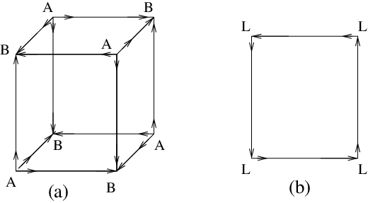
In (90), l→[i​j],p→[i1​i2​i3],q→[j1​j2​j3]\vec{l}_{[ij]},\vec{p}_{[i_{1}i_{2}i_{3}]},\vec{q}_{[j_{1}j_{2}j_{3}]} are 2​d​(2​d−1)​(2​d+1)3\frac{2d(2d-1)(2d+1)}{3} non-negative integers describing all possible SU(3) gauge invariant states at a given lattice site. The various possible loop states set in pure SU(3) lattice gauge theory are direct products of (90) at various lattice sites consistent with U⁡(1)⊗U⁡(1)U(1)\otimes U(1) Gauss law (46) along every link.

As in the loop formulation where various loop states are mutually related by Mandelstam constraints, not all states in (90) are linearly independent. Infact, in the present SU(3) prepotential formulation (like in SU(2) case) the Mandelstam constraints become local and take very simple forms in terms of the SU(3) gauge invariant vertices in (87,88) and (89) at every lattice site n. We start with the simplest SU(3) Mandelstam constraints:

A[i1,i2,i3]​B[j1,j2,j3]≡∑{s1,s2,s3}∈S3(−1)s​L[i1​js1]​L[i2​js2]​L[i3​js3].\displaystyle A_{[i_{1},i_{2},i_{3}]}B_{[j_{1},j_{2},j_{3}]}\equiv\sum_{\{s_{1},s_{2},s_{3}\}\in S_{3}}(-1)^{s}L_{[i_{1}j_{s_{1}}]}L_{[i_{2}j_{s_{2}}]}L_{[i_{3}j_{s_{3}}]}. (91)
Refer to caption
Figure 9: The graphical representation of local SU(3) Mandelstam constraints (91) in terms of SU(3) gauge invariant vertices A,BA,B and LL constructed out of the SU(3) irreducible prepotential operators at a lattice site n. The A and B type of vertices at n annihilate each other to produce L type of vertices.

In (91), S3S_{3} denotes the permutation group of order 3, {s1,s2,s3}\{s_{1},s_{2},s_{3}\} denote the 3!3! permutations of {1,2,3}\{1,2,3\} and ss is the parity of permutation. In other words, the Mandelstam constraints (91) state that the A and B type vertices annihilate each other in pairs to produce L type vertices. The constraints (91) are illustrated in Figure 9. Therefore, the SU(3) gauge invariant states of (L−A−B)(L-A-B) type in (90) can always be written either as (L−A)(L-A) type or as (L−B)(L-B) type at each lattice site. It is interesting to analyze the Mandelstam constraints discussed in [4] in terms of SU(3) prepotential operators. Following [4], we consider the set of r (r>3)(r>3) loops C1​(n),C2​(n),⋯,Cr​(n)C_{1}(n),~C_{2}(n),\cdots,C_{r}(n) all based at lattice site n. These loops start from n in the direction i1,i2,⋯iri_{1},i_{2},\cdots i_{r} and come back to n from directions j1,j2,⋯jrj_{1},j_{2},\cdots j_{r} respectively. Then the products of these Wilson loops satisfies:

∑αi1⋯αirβj1⋯βjrϵαi1αi2⋯αirϵβj1βj2⋯βjr(W(C1(n))αj1(W(C2(n))αj2⋯βi2(W(Cr(n))αjr≡βir0.βi1\displaystyle\sum_{{}^{\alpha_{i_{1}}\cdots\alpha_{i_{r}}}_{\beta_{j_{1}}\cdots\beta_{j_{r}}}}\epsilon_{\alpha_{i_{1}}\alpha_{i_{2}}\cdots\alpha_{i_{r}}}\epsilon^{\beta_{j_{1}}\beta_{j_{2}}\cdots\beta_{j_{r}}}\left(W(C_{1}(n)\right)^{\alpha_{j_{1}}}{}_{\beta_{i_{1}}}\left(W(C_{2}(n)\right)^{\alpha_{j_{2}}}{}_{\beta_{i_{2}}}\cdots\left(W(C_{r}(n)\right)^{\alpha_{j_{r}}}{}_{\beta_{i_{r}}}\equiv 0. (92)

Using the identities

ϵαi1αi2⋯αirϵβj1βj2⋯βjr=δβj1αi1δβj2αi2⋯δβjrαir−δβj1αi2δβj2αii⋯δβjrαir+⋯\epsilon_{\alpha_{i_{1}}\alpha_{i_{2}}\cdots\alpha_{i_{r}}}\epsilon^{\beta_{j_{1}}\beta_{j_{2}}\cdots\beta_{j_{r}}}=\delta^{\beta_{j_{1}}}_{\alpha_{i_{1}}}\delta^{\beta_{j_{2}}}_{\alpha_{i_{2}}}\cdots\delta^{\beta_{j_{r}}}_{\alpha_{i_{r}}}-\delta^{\beta_{j_{1}}}_{\alpha_{i_{2}}}\delta^{\beta_{j_{2}}}_{\alpha_{i_{i}}}\cdots\delta^{\beta_{j_{r}}}_{\alpha_{i_{r}}}+\cdots

(93) can be written in terms of traces of Wilson loops [4]:

TrW(C1)TrW(C2)⋯TrW(Cr)−TrW(C1C2)TrW(C3)TrW(C4)⋯TrW(Cr)+⋯=0.\displaystyle TrW(C_{1})TrW(C_{2})\cdots TrW(C_{r})-TrW(C_{1}C_{2})TrW(C_{3})TrW(C_{4})\cdots TrW(C_{r})+\cdots=0. (93)

The Mandelstam constraints (93) in terms of the link operators represent highly non-local constraints as one can always choose the loops C1,C2,⋯CrC_{1},C_{2},\cdots C_{r} to be as large as one wishes. However, in terms of the prepotentials the constraints (93) become local. All one has to do is to replace the Wilson loops in (93) by the prepotentials which are attached to their starting and end points, i.e,:

W(Cs)αis→βisLαjs≡βisB†αjsAβis†,s=1,2,⋯,r.\displaystyle W(C_{s})^{\alpha_{i_{s}}}{}_{\beta_{i_{s}}}\rightarrow L^{\alpha_{j_{s}}}{}_{\beta_{i_{s}}}\equiv B^{\dagger\alpha_{j_{s}}}A^{\dagger}_{\beta_{i_{s}}},~~s=1,2,\cdots,r. (94)

Note that unlike non-local Wilson loop W⁡(Cs)W(C_{s}), the operators BαjsB^{\alpha_{j_{s}}} and Aβis†A^{\dagger}_{\beta_{i_{s}}} and hence LαjsβisL^{\alpha_{j_{s}}}{}_{\beta_{i_{s}}} are completely defined at lattice site n. Noting that Tr(Lαjs)βis=L[isjs]Tr\left(L^{\alpha_{j_{s}}}{}_{\beta_{i_{s}}}\right)=L[i_{s}j_{s}], the non-local Mandelstam constraints (93) acquire the following simple local form:

∑{s1,s2,⋯sr}∈Sr(−1)sL[i1​js1]L[i2​js2]⋯L[i3​jsr]=0\displaystyle\sum_{\{s_{1},s_{2},\cdots s_{r}\}\in S_{r}}(-1)^{s}L_{[i_{1}j_{s_{1}}]}L_{[i_{2}j_{s_{2}}]}\cdots L_{[i_{3}j_{s_{r}}]}=0 (95)

and are illustrated in Figure 10. Note that all the unnecessary details like shapes, sizes and lengths of the loops C1,C2,⋯CrC_{1},C_{2},\cdots C_{r} in (93) disappear in the corresponding prepotential form (95).

Refer to caption
Figure 10: The graphical representation of local SU(3) Mandelstam constraints (95) involving only LL type of vertices at lattice site n.

4.6.1 The solutions

The Mandelstam constraints in their present local prepotential forms (91) and (95), instead of non-local form (93) in terms of link operators, are now accessible to explicit local solutions like in SU(2) lattice gauge theory [8]. Note that they are still infinite in number at every lattice site. The solutions must be all possible mutually independent linear combinations of the states in (90) at a given lattice site. Following the techniques discussed in [10] in the context of duality transformations in lattice gauge theories, these linear combinations can be obtained by characterizing the resultant states at a site n by their complete SU(3) quantum numbers with the net SU(3) fluxes being zero. This will be SU(3) analogue of SU(2) result (40). The quantum numbers needed to specify such states can be easily computed [10] as follows. In d dimension, there are 2d links emanating from a lattice site n. Each of these 2d directions is attached with SU(3) operators (A†​[i],B†​[i],i=1,2,⋯,2​d)(A^{\dagger}[i],B^{\dagger}[i],i=1,2,\cdots,2d) as shown in Figure 7. Therefore, there are 2d Hilbert spaces associated with a lattice site and each can be characterized by it’s SU(3) quantum numbers. In the standard language [24], the SU(3) irreducible representations are completely specified by 5 quantum numbers: |p,q,i2,iz,y⟩|p,q,i^{2},i_{z},y\rangle where p and q are the eigenvalues of two SU(3) Casimir operators and i,iz,yi,i_{z},y are the SU(3) “magnetic” quantum numbers representing SU(2) spin, it’s third component and hyper charge respectively. In the present language with constraints, each of the 2d directions (see Figure 7) is associated with 6 harmonic oscillators (A†​[i],B†​[i],i=1,2,⋯,2​d)(A^{\dagger}[i],B^{\dagger}[i],i=1,2,\cdots,2d) and therefore requires 6 occupation numbers to completely specify the basis. The constraints k−[i]≡a[i]⋅b[i]≃0k_{{}_{-}}[i]\equiv a[i]\cdot b[i]\simeq 0 reduces this to 5 in each direction. Therefore 5×2​d=10​d5\times 2d=10d quantum numbers are needed to specify a local Hilbert space basis completely at each lattice site. Not all these quantum numbers are independent as 2d of these are related to the previous sites by U⁡(1)⊗U⁡(1)U(1)\otimes U(1) Gauss law constraints (46). Therefore, we are left with 8​d8d quantum numbers at every lattice site. Finally, the SU(3) gauge invariance further implies 8 constraints. Therefore, the net independent quantum numbers are 8​(d−1)8(d-1) per lattice site. As expected, this is the the number of transverse degree of freedom of 8 SU(3) gluons in d dimension at every lattice site. The abelian U⁡(1)×U⁡(1)U(1)\times U(1) fluxes over the links will now glue these local SU(3) invariant orthogonal basis at neighboring lattice sites according to their Gauss laws (46). This will give complete solutions of all the SU(3) Mandelstam constraints like what what was done in SU(2) lattice gauge theory [8]. Infact, the addition of fluxes in SU(3) lattice gauge theory has been discussed in [27]). These results combined with the results of this work should enable us to solve SU(3) Mandelstam constraints completely in terms of vertex operators of section (4.6). This explicit construction of all the independent SU(3) loop states and their dynamics along the line of [8] is in progress and will be reported elsewhere.

5 Summary and discussion

In this work we analyze SU(3) lattice gauge theory in terms of the prepotential operators which under gauge transformations transform like fundamental matter fields. We constructed the SU(3) irreducible prepotential operators which acting on strong coupling vacuum directly created the QCD fluxes around lattice sites. All SU(3) gauge invariant vertices in terms of these QCD flux operators were constructed at every lattice site. These SU(3) invariant vertices, in turn, enabled us to cast all SU(3) Mandelstam constraints in their local forms. As mentioned in the text this is an essential step towards their complete solution. The complete solution of Mandelstam constraints, in turn, will allow us to write down SU(3) lattice gauge theory completely and exactly in terms of minimum essential gauge invariant loop and string co-ordinates without any redundant loop/strings degrees of freedom. The prepotential operators also allow us to simplify lattice gauge theory Hamiltonian as given in (1). In particular, for the present SU(3) case, one can simply replace the plaquette or magnetic term T​r​Up​l​a​q​u​e​t​t​eTrU_{plaquette} in (1) by a new plaquette interaction consisting of the 4 L type vertices at the 4 corners of every plaquette. Note that the new Hamiltonian constructed this was has exactly the same symmetries as (1) and therefore expected to be in the same universality class. The addition of matter field interactions in the prepotential formulation is trivial as matter and prepotential have similar SU(3) gauge transformation properties. The difference lies in the abelian U⁡(1)⊗U⁡(1)U(1)\otimes U(1) transformations under which matter fields remain invariant.

The results in this work can also be generalized to SU(N) lattice gauge theory. We can use SU(N) Schwinger bosons [26] or prepotentials to construct SU(N) electric fields on lattice similar to (11) and (41). We need to elevate these prepotentials so that they have symmetries of SU(N) Young tableaues inbuilt. As in section (4.6), the SU(N) Mandelstam constraints will again be local and can be solved using the techniques discussed in this work. The work in this direction is in progress and will be reported elsewhere.

Acknowledgment One of the authors (M.M.) would like to thank H. S. Sharatchandra for many interesting discussions during the course of this work.

Appendix A The projection operators in ℋp{\cal H}_{p}:

In this appendix we briefly discuss the construction of projection operators which project ℋp{\cal H}_{p} to ℋg{\cal H}_{g} on every link:

𝒫​{ℋp}l​i​n​k={ℋp​(ρ=0)}l​i​n​k={ℋg}l​i​n​k.\displaystyle{\cal P}~\left\{{\cal H}_{p}\right\}_{link}=\left\{{\cal H}_{p}(\rho=0)\right\}_{link}=\left\{{\cal H}_{g}\right\}_{link}. (96)

The group theoretical details of this construction can be found in [22]. It is convenient to first break up {ℋp}l​i​n​k\left\{{\cal H}_{p}\right\}_{link} into Hilbert spaces containing p (q) quarks and q (p) anti-quark prepotentials on the left (right):

{ℋp}l​i​n​k=∑p,q=0∞⊕{ℋp}l​i​n​k(p,q).\displaystyle\left\{{\cal H}_{p}\right\}_{link}=\sum_{p,q=0}^{\infty}\oplus\left\{{\cal H}_{p}\right\}_{link}(p,q). (97)

These subspaces {ℋp}l​i​n​k​(p,q)\left\{{\cal H}_{p}\right\}_{link}(p,q) are themselves direct products of left and right Hilbert spaces:

{ℋp}l​i​n​k​(p,q)={ℋpL}l​i​n​k​(p,q)⊗{ℋpR}l​i​n​k​(q,p).\displaystyle\left\{{\cal H}_{p}\right\}_{link}(p,q)=\left\{{\cal H}_{p}^{L}\right\}_{link}(p,q)\otimes\left\{{\cal H}_{p}^{R}\right\}_{link}(q,p). (98)

The basis vectors spanning {ℋpl}l​i​n​k​(p,q),l=L,R\left\{{\cal H}_{p}^{l}\right\}_{link}(p,q),l=L,R are given in terms of left and right flux creation operators:

L^α1α2⋯αpβ1β2⋯βq|0⟩L≡aα1†(L)⋯aαp†(L)b†β1(L)⋯b†βq(L)|0⟩L,\hat{L}_{\alpha_{1}\alpha_{2}\cdots\alpha_{p}}^{\beta_{1}\beta_{2}\cdots\beta_{q}}|0\rangle_{L}~\equiv~a^{\dagger}_{\alpha_{1}}(L)\cdots a^{\dagger}_{\alpha_{p}}(L)b^{\dagger\beta_{1}}(L)\cdots b^{\dagger\beta_{q}}(L)|0\rangle_{L},

and

R^γ1γ2⋯γqδ1δ2⋯δp|0⟩R≡aγ1†(R)⋯aγq†(R)b†δ1(R)⋯b†δp(R)|0⟩R\hat{R}_{\gamma_{1}\gamma_{2}\cdots\gamma_{q}}^{\delta_{1}\delta_{2}\cdots\delta_{p}}|0\rangle_{R}~\equiv~a^{\dagger}_{\gamma_{1}}(R)\cdots a^{\dagger}_{\gamma_{q}}(R)b^{\dagger\delta_{1}}(R)\cdots b^{\dagger\delta_{p}}(R)|0\rangle_{R}

in (47). We now construct the projection operators 𝒫l​(p,q){\cal P}_{l}(p,q) in each of these subspaces with

𝒫=∑p,q=0∞⊕𝒫L(p,q)⊗𝒫R(q,p).\displaystyle{\cal P}=\sum_{p,q=0}^{\infty}\oplus{\cal P}_{L}(p,q)\otimes{\cal P}_{R}(q,p). (99)

The left and right projection operators 𝒫l​(p,q),l=L,R{\cal P}_{l}(p,q),l=L,R are of the form [22]:

𝒫L​(p,q)\displaystyle{\cal P}_{L}(p,q) ≡\displaystyle\equiv ∑r=0∞gr​(p,q)​(k+​(L))r​(k−​(L))r\displaystyle\sum_{r=0}^{\infty}g_{r}(p,q)\left(k_{+}(L)\right)^{r}\left(k_{-}(L)\right)^{r}
𝒫R​(q,p)\displaystyle{\cal P}_{R}(q,p) ≡\displaystyle\equiv ∑r=0∞hr​(q,p)​(k+​(R))r​(k−​(R))r\displaystyle\sum_{r=0}^{\infty}h_{r}(q,p)\left(k_{+}(R)\right)^{r}\left(k_{-}(R)\right)^{r} (100)

The unknown coefficients g and h in (100) are fixed by demanding the Sp(2,R) constraints (57):

k−​(L)​𝒫L​(p,q)​{ℋpL}l​i​n​k​(p,q)=0,k−​(R)​𝒫R​(q,p)​{ℋpR}l​i​n​k​(q,p)=0.\displaystyle k_{-}(L){\cal P}_{L}(p,q)\left\{{\cal H}_{p}^{L}\right\}_{link}(p,q)=0,~~~~k_{-}(R){\cal P}_{R}(q,p)\left\{{\cal H}_{p}^{R}\right\}_{link}(q,p)=0. (101)

The solutions of the equations (101) are [22]:

gr​(p,q)=hr​(q,p)=(−1)rr!​(p+q+1−r)!(p+q+1)!,\displaystyle g_{r}(p,q)=h_{r}(q,p)=\frac{(-1)^{r}}{r!}\frac{(p+q+1-r)!}{(p+q+1)!}, (102)

leading to:

𝒫L​(p,q)\displaystyle{\cal P}_{L}{(p,q)} =\displaystyle= 1(p+q+1)!​∑r=0∞(−1)rr!​(p+q+1−r)!​(k+​(L))r​(k−​(L))r,\displaystyle\frac{1}{(p+q+1)!}\sum_{r=0}^{\infty}\frac{(-1)^{r}}{r!}({p}+{q}+1-r)!\left(k_{+}(L)\right)^{r}\left(k_{-}(L)\right)^{r},
𝒫R​(q,p)\displaystyle{\cal P}_{R}{(q,p)} =\displaystyle= 1(p+q+1)!​∑r=0∞(−1)rr!​(p+q+1−r)!​(k+​(R))r​(k−​(R))r.\displaystyle\frac{1}{(p+q+1)!}\sum_{r=0}^{\infty}\frac{(-1)^{r}}{r!}({p}+{q}+1-r)!\left(k_{+}(R)\right)^{r}\left(k_{-}(R)\right)^{r}. (103)

Note that the SU(3) irreducible prepotentials in (61) already commute with the Sp(2,R) constraints (62) and therefore acting on the strong coupling vacuum directly generate the gauge theory Hilbert space ℋg{\cal H}_{g}. In other words:

ℒ^α1α2⋯αpβ1β2⋯βq|0⟩L=𝒫L(p,q)L^α1α2⋯αpβ1β2⋯βq|0⟩L,ℛ^γ1γ2⋯γqδ1δ2⋯δp|0⟩R.=𝒫R(q,p)R^γ1γ2⋯γqδ1δ2⋯δp|0⟩R\displaystyle\hat{{\cal L}}_{~\alpha_{1}\alpha_{2}\cdots\alpha_{p}}^{~\beta_{1}\beta_{2}\cdots\beta_{q}}|0\rangle_{L}={\cal P}_{L}(p,q)\hat{{L}}_{~\alpha_{1}\alpha_{2}\cdots\alpha_{p}}^{~\beta_{1}\beta_{2}\cdots\beta_{q}}|0\rangle_{L},~~~~\hat{{\cal R}}_{~\gamma_{1}\gamma_{2}\cdots\gamma_{q}}^{~\delta_{1}\delta_{2}\cdots\delta_{p}}|0\rangle_{R}.={\cal P}_{R}(q,p)\hat{{R}}_{~\gamma_{1}\gamma_{2}\cdots\gamma_{q}}^{~\delta_{1}\delta_{2}\cdots\delta_{p}}|0\rangle_{R} (104)

are the relations amongst the SU(3) reducible and irreducible flux operators on the left and right side of every link.

Appendix B The electric field constraints

Using the λ\lambda matrix identity: ∑a=18(λa2)βα​(λa2)σγ=12​δσα​δβγ−16​δβα​δσγ\sum_{a=1}^{8}\left(\frac{\lambda^{a}}{2}\right)^{\alpha}_{\beta}\left(\frac{\lambda^{a}}{2}\right)^{\gamma}_{\sigma}=\frac{1}{2}\delta^{\alpha}_{\sigma}\delta^{\gamma}_{\beta}-\frac{1}{6}\delta^{\alpha}_{\beta}\delta^{\gamma}_{\sigma}, the squares of left and right electric fields can be written as:

∑a=18ELa​(n,i)​ELa​(n,i)\displaystyle\sum_{a=1}^{8}E_{L}^{a}(n,i)E_{L}^{a}(n,i) =\displaystyle= N^​(L)​(N^​(L)3+1)+M^​(L)​(M^​(L)3+1)−k+​(L)​k−​(L)+13​N^​(L)​M^​(L)\displaystyle\hat{N}(L)\left(\frac{\hat{N}(L)}{3}+1\right)+\hat{M}(L)\left(\frac{\hat{M}(L)}{3}+1\right)-~k_{+}(L)k_{-}(L)+\frac{1}{3}\hat{N}(L)\hat{M}(L)
∑a=18ERa​(n,i)​ERa​(n,i)\displaystyle\sum_{a=1}^{8}E_{R}^{a}(n,i)E_{R}^{a}(n,i) =\displaystyle= N^​(R)​(N^​(R)3+1)+M^​(R)​(M^​(R)3+1)−k+​(R)​k−​(R)+13​N^​(R)​M^​(R).\displaystyle\hat{N}(R)\left(\frac{\hat{N}(R)}{3}+1\right)+\hat{M}(R)\left(\frac{\hat{M}(R)}{3}+1\right)-k_{+}(R)k_{-}(R)+\frac{1}{3}\hat{N}(R)\hat{M}(R).

The electric field constraints (6) along with the U⁡(1)⊗U⁡(1)U(1)\otimes U(1) Gauss law constraints (46) imply:

k+​(L)​k−​(L)=k+​(R)​k−​(R).\displaystyle k_{+}(L)k_{-}(L)=k_{+}(R)k_{-}(R). (105)

On the other hand, the action of k+​k−k_{+}k_{-} on a general Sp(2,R) irrep. |k,m⟩|k,m\rangle is given by [21]:

k+k−|k,m⟩=(m−k)(m+k−1)|k,m⟩,\displaystyle k_{+}k_{-}|k,m\rangle=(m-k)(m+k-1)|k,m\rangle, (106)

where, m=k+ρm=k+\rho. In the present case the electric field constraint (B) and the eigenvalue equation (106) imply:

(m⁡(L)−k⁡(L))​(m⁡(L)+k⁡(L)−1)=(m⁡(R)−k⁡(R))​(m⁡(R)+k⁡(R)−1).\displaystyle\left(m(L)-k(L)\right)\left(m(L)+k(L)-1\right)=\left(m(R)-k(R)\right)\left(m(R)+k(R)-1\right). (107)

As k⁡(L)=k⁡(R)=12​(p+q+3)k(L)=k(R)=\frac{1}{2}(p+q+3), we get the unique solution of (107):

ρL​(n,i)=ρR​(n+i,i).\displaystyle\rho_{L}(n,i)=\rho_{R}(n+i,i). (108)

Therefore, in the prepotential Hilbert space ℋp{\cal H}_{p} the left and the right Sp(2,R) “magnetic” quantum numbers are same on every link.

References

  • [1] S. Mandelstam, Ann. Phys. (N.Y.) 19 (1962) 1; S. Mandelstam, Phys. Rev. 175 (1968) 1580; S. Mandelstam, Phys. Rev. D 19 (1979) 2391.
  • [2] K. G. Wilson, Phys. Rev. D 10 (1974) 2445.
  • [3] A. M. Polyakov, Phys. Lett. B 82 (1979) 247; (1983) 199; A. M. Polyakov, Nucl. Phys. B164 (1979) 171; N. Nambu, Phys. Lett. B 80 (1979) 372; J. L. Gervais, A. Neveu, Phys. Lett. B 80 (1979) 255; Yu. M. Makeenko and A. A. Migdal, Phys. Lett. B88 (1979) 135; Y. M. Makeenko, A. A. Migdal, Nucl. Phys. B 188 (1981) 269; F. Gliozzi, T. Reggeand M. A. Virasaro, Phys. Lett. B81 (1979) 178; M. Virasaro, Phys. Lett. B 82 (1979) 436; A. Jevicki and B. Sakita, Phys. Rev. D 22 (1974) 467; A. M. Polyakov, Gauge Fields and Strings (Harwood, New York, 1987).
  • [4] A. A. Migdal, Phys. Rep. 102 199-290 (1983).
  • [5] J. Kogut, L Susskind, Phys Rev. D 10 (1974) 3468, D 11, 395 (1975).
  • [6] R. Gambini, Jorge Pullin, Loops, Knots, Gauge Theories and Quantum Gravity (Cambridge University Press, 2000).
  • [7] As emphasized in [6]: “The proliferation of loops when one considers larger lattices and higher dimensions completely washes out the advantages provided by the (loop) formalism.”, Chapter 12, page 303-304; Gambini R, Leal L, Trias A, Phys. Rev. D 39 (1989) 3127; Bartolo C, Gambini R, Leal L, Phys. Rev. D 39 (1989) 1756.
  • [8] Manu Mathur, Nucl. Phys. B 779, 32 (2007), Phys. Letts. B 640 (2006) 292-296.
  • [9] Manu Mathur, J. Phys. A: Math. Gen. 38 (2005) 10015.
  • [10] H. S. Sharatchandra, Nucl. Phys. B 196 (1982) 62.
  • [11] Ramesh Anishetty, H. S. Sharatchandra, Phys. Rev. Letts. 65 (1990) 81; B. Gnanapragasam, H. S. Sharatchandra, Phys. Rev. D 45 (1992) R1010;
  • [12] D. Robson, D. M. Weber, Z. Phys. C15 (1982) 199.
  • [13] W. Furmanski, A. Kolawa, Nucl. Phys. B 291 (1987) 594.
  • [14] G. Burgio, R. De. Pietri, H. A. Morales-Tecotl, L. F. Urrutia, J. D. Vergara, Nucl. Phys. B 566 (2000), 547.
  • [15] Brügmann B, Phys. Rev. D 43 (1991) 566.
  • [16] Loll R. Nucl. Phys B 368 (1992) 121, Nucl. Phys. B 400 (1993) 126.
  • [17] Watson N. J., Phys. Letts. B 323 (1994) 385; Nucl. Phys. Proc. Suppl. (1995) 39B, C 224, hep-th/9408174.
  • [18] C. Rovelli, Quantum Gravity, Cambridge University Press (2004).
  • [19] C. Rovelli, L. Smolin, Phys. Rev. D 52 (1995) 5743, [arXiv:gr-qc/9505006].
  • [20] N. D. H. Dass and Manu Mathur, Class. Quant. Grav. 24, 2179 (2007) [arXiv:gr-qc/0611156].
  • [21] S. Chaturvedi and n. Mukunda, J. Math. Phys. 43 (2002) 5262
  • [22] Ramesh Anishetty, Manu Mathur and Indrakshi Raychowdhury, J. Math. Phys. 50 (2009) 053503.
  • [23] P. Jordan, Z. Physik 94 (1935) 531, J. Schwinger U.S Atomic Energy Commission Report NYO-3071, 1952 or D. Mattis, The Theory of Magnetism (Harper and Row, 1982).
  • [24] H. Georgi, Lie Algebras in Particle Physics (Benjamin/Cummings, Reading, 1982).
  • [25] Manu Mathur and Diptiman Sen, J. Math. Phys. 42 (2001) 4181.
  • [26] Manu Mathur and H. S. Mani, J. Math. Phys. 43 (2002) 5351.
  • [27] R. Anishetty, H. Gopalkrishna Gadiyar, Manu Mathur and H. S. Sharatchandra, Phys. Lett. B 271, (1991) 391; J. S. Prakash and H. S. Sharatchandra, J. Math. Phys. 37, (1996) 6530.