Equation of State and Heavy-Quark Free Energy at Finite Temperature and Density in Two Flavor Lattice QCD with Wilson Quark Action

Preprint: TKYNT-09-18, UTHEP-589, 2009/September

S. Ejiri¹, Y. Maezawa², N. Ukita³, S. Aoki^4,5, T. Hatsuda⁶, N. Ishii⁶, K. Kanaya⁴ and T. Umeda⁷
(WHOT-QCD Collaboration) Affiliation: ¹Physics Department, Brookhaven National Laboratory, Upton, New York 11973, USA
²En’yo Laboratory, Nishina Accelerator Research Center, RIKEN, Wako 351-0198, Japan
³Center for Computational Sciences, University of Tsukuba, Tsukuba, Ibaraki 305-8577, Japan
⁴Graduate School of Pure and Applied Sciences, University of Tsukuba, Tsukuba, Ibaraki 305-8571, Japan
⁵RIKEN BNL Research Center, Brookhaven National Laboratory, Upton, New York 11973, USA
⁶Department of Physics, The University of Tokyo, Tokyo 113-0033, Japan
⁷Graduate School of Education, Hiroshima University, Hiroshima 739-8524, Japan

June 30, 2010

Abstract

We study the equation of state at finite temperature and density in two-flavor QCD with the RG-improved gluon action and the clover-improved Wilson quark action on a $16^{3}\times 4$ lattice. Along the lines of constant physics at $m_{\rm PS}/m_{\rm V}=0.65$ and 0.80, we compute the second and forth derivatives of the grand canonical partition function with respect to the quark chemical potential $\mu_{q}=(\mu_{u}+\mu_{d})/2$ and the isospin chemical potential $\mu_{I}=(\mu_{u}-\mu_{d})/2$ at vanishing chemical potentials, and study the behaviors of thermodynamic quantities at finite $\mu_{q}$ using these derivatives for the case $\mu_{I}=0$ . In particular, we study density fluctuations at nonezero temperature and density by calculating the quark number and isospin susceptibilities and their derivatives with respect to $\mu_{q}$ . To suppress statistical fluctuations, we also examine new techniques applicable at low densities. We find a large enhancement in the fluctuation of quark number when the density increased near the pseudo-critical temperature, suggesting a critical point at finite $\mu_{q}$ terminating the first order transition line between hadronic and quark gluon plasma phases. This result agrees with the previous results using staggered-type quark actions qualitatively. Furthermore, we study heavy-quark free energies and Debye screening masses at finite density by measuring the first and second derivatives of these quantities for various color channels of heavy quark-quark and quark-anti-quark pairs. The results suggest that, to the leading order of $\mu_{q}$ , the interaction between two quarks becomes stronger at finite densities, while that between quark and anti-quark becomes weaker.

pacs

11.15.Ha, 12.38.Gc, 12.38.Mh

I Introduction

Heavy-ion collision experiments are taking place at BNL aiming at the experimental studies of a new state of matter, the quark-gluon plasma [1]. In order to extract unambiguous signals for the QCD phase transition from the heavy-ion collision experiments, quantitative calculations directly from the first principles of QCD are indispensable. At present, the lattice QCD simulation is the only systematic method to do so. Various computational techniques have been developed to study the nature of quark matter at finite temperature $(T)$ and at small chemical potentials $\mu_{u}$ and $\mu_{d}$ [2, 3]. From intensive studies for the isosymmetric case $\mu_{u}=\mu_{d}=\mu_{q}$ , it turned out that accurate zero-temperature simulations are important to set the scale to achieve high precision results at finite $T$ and $\mu_{q}$ .

Most of the lattice QCD studies at finite $\mu_{q}$ so far have been performed using staggered-type quark actions with the fourth-root trick for the quark determinant. However, the fourth-root trick makes the theory non-local and thus the universality arguments fragile. It should be kept in mind that the staggered-type quarks for two-favor QCD does not show the scaling properties at finite $T$ expected from the three-dimensional O(4) spin model [4, 5]. This may suggest large lattice artifacts to the results of staggered-type quarks near the transition point. Moreover, problems in the staggered quark formulation at finite density are pointed out in [6]. Since the theoretical base for the fourth-root trick is not clear, it is indispensable to carry out simulations adopting different lattice quark actions to control and estimate systematic errors due to the lattice discretization.

Several years ago, the CP-PACS Collaboration has studied finite-temperature QCD using the clover-improved Wilson quark action coupled with the RG-improved Iwasaki action for gluons [7, 8]. With two flavors of dynamical quarks, the phase structure, the transition temperature and the equation of state have been investigated. In contrast to the case of the staggered-type quarks, both the standard Wilson quark action [9] and the clover-improved Wilson quark action [7] reproduce the expected universality around the critical point of the chiral phase transition: the subtracted chiral condensate shows the scaling behavior with the critical exponents and scaling function of the three-dimensional O(4) spin model. Moreover, extensive calculations of major physical quantities such as the light hadron masses have been carried out at $T=0$ using the same action [10, 11]. Therefore, it is worth revisiting this action armed with recent techniques for finite $\mu_{q}$ .

In the $(T,\mu_{q})$ plane, phenomenological studies suggest the existence of a critical point at which the first order phase transition line separating the hadronic phase and the quark-gluon-plasma phase terminates [12, 13, 14]. Because the critical point has second order characteristics, the fluctuation of the net quark number will diverge as we approach to the critical point in the $(T,\mu_{q})$ plane, while the fluctuation in the isospin number will remain finite [15, 16]. Such hadronic fluctuations may be experimentally examined in heavy-ion collisions by an event-by-event analysis. The Bielefeld-Swansea Collaboration reported lattice results for the quark number susceptibility (the second derivative of the thermodynamic grand canonical potential $\omega/T^{4}=-(VT^{3})^{-1}\ln{\cal Z}$ , which is proportional to the pressure of the system) by the Taylor expansion method using a p4-improved staggered quark action [17, 18, 19]: From a calculation of the Taylor expansion coefficients of $\omega/T^{4}$ up to $O[(\mu_{q}/T)^{6}]$ , they found that the quark number fluctuation increases rapidly as $\mu_{q}$ increases in the region near the transition temperature. This suggests indirectly the existence of the nearby critical point in the $(T,\mu_{q})$ plane. Moreover, 2+1 flavor simulations in staggered quarks with almost physical quark masses have recently been performed and the same behaviors in the fluctuations have been found at finite density [20, 21]. Therefore, it is important to confirm the result using the Wilson-type quarks.

In this paper, we study thermodynamic properties of QCD at finite temperature and density with two flavors of clover-improved Wilson quarks coupled with the RG-improved Iwasaki gluons. The simulations are performed along lines of constant physics corresponding to the pion and rho meson mass ratio, $m_{\rm PS}/m_{\rm V}=0.65$ and 0.80 at $T=0$ . We calculate the Taylor coefficients for the pressure in terms of $\mu_{q}/T$ up to the fourth order, and study the quark number and isospin susceptibilities at finite $\mu_{q}$ . Since the odd derivatives vanish at $\mu_{q}=0$ , the fourth derivative is the leading contribution to the $\mu_{q}$ -dependence of susceptibilities. We find that Wilson-type quarks require much more statistics than staggered-type quarks to obtain the susceptibilities with a comparable quality. To overcome this problem, we introduce a couple of tricks in the evaluation of the Taylor expansion coefficients. Furthermore, we adopt a hybrid method of Taylor expansion and spectral reweighting in which $\omega/T^{4}$ for the reweighting is approximated by a truncated Taylor expansion [22, 18]. Since the applicable range of the reweighting method is narrow due to the sign problem, we introduce the Gaussian method proposed in [23]. Using these techniques, we compute the quark number density and the susceptibility in a relatively wide range of $\mu_{q}/T$ , and compare the results with those with staggered-type quarks.

We also extend our previous study of heavy-quark free energies in various color channels at $\mu_{q}=0$ [24] to finite $\mu_{q}$ . At $T>T_{pc}$ , where $T_{pc}$ is the pseudo-critical temperature, we calculate the Taylor expansion coefficients for the heavy-quark free energies between a static quark ( $Q$ ) and an antiquark ( $\bar{Q}$ ) and those between $Q$ and $Q$ , for all color channels up to the second order in $\mu_{q}/T$ . By comparing the expansion coefficients of the free energies, we find that the inter-quark interaction between $Q$ and $\bar{Q}$ becomes weaker, whereas that between $Q$ and $Q$ becomes stronger as $\mu_{q}$ increases. The expansion coefficients of the effective running coupling $\alpha_{\rm eff}(T,\mu_{q})$ and the Debye screening mass $m_{D}(T,\mu_{q})$ are also extracted by fitting the numerical results with a screened Coulomb form; we find that the heavy-quark free energies are well reproduced by the channel dependent Casimir factor and the channel independent $\alpha_{\rm eff}(T,\mu_{q})$ and $m_{D}(T,\mu_{q})$ at $T\mathrel{\hbox to0.0pt{\raise 2.20013pt\hbox{$>$}\hss}{\lower 2.20013pt\hbox{$\sim$}}}2T_{pc}$ . Magnitude of the second order coefficient of $m_{D}(T,\mu_{q})$ does not agree with that of the leading-order calculation in the thermal perturbation theory.

In Sec. II, we summarize our lattice action and simulation parameters, and determine the pseudo-critical temperature. In Sec. III, we calculate the Taylor expansion coefficients of the thermodinamic grand canonical potenital in terms of the quark chemical potentials $\mu_{u}$ and $\mu_{d}$ and evaluate them for the isosymmetric case $\mu_{u}=\mu_{d}=\mu_{q}$ at $\mu_{q}=0$ up to $O(\mu_{q}^{4})$ . In Sec. IV, we adopt the hybrid method combined with the Gaussian method, to improve the calculation. The static quark free energies and the Debye screening mass are discussed in Sec. V. Conclusions and discussions are given in Sec. VI. We summarize properties of the pressure and the quark number susceptibility in the free gas limit in Appendix A. Appendix B is devoted to a description of detailed derivations of formulae for the Gaussian method. Results of the fits of heavy-quark free energies are summarized in Appendix C.

II Phase structure and lines of constant physics at $\mu_{q}=0$

II.1 Lattice action

First, we summarize our simulation details. We adopt the same lattice actions as in our previous study at $\mu_{q}=0$ [24]. We use the RG-improved Iwasaki gauge action [25] and the $N_{f}=2$ clover-improved Wilson quark action [26] defined by

$\displaystyle S$	$\displaystyle=$	$\displaystyle S_{g}+S_{q},$	(1)
$\displaystyle S_{g}$	$\displaystyle=$	$\displaystyle-{\beta}\sum_{x}\left(c_{0}\sum_{\mu<\nu;\mu,\nu=1}^{4}W_{\mu\nu}^{1\times 1}(x)+c_{1}\sum_{\mu\neq\nu;\mu,\nu=1}^{4}W_{\mu\nu}^{1\times 2}(x)\right),$	(2)
$\displaystyle S_{q}$	$\displaystyle=$	$\displaystyle\sum_{f=u,d}\sum_{x,y}\bar{\psi}_{x}^{f}M_{x,y}\psi_{y}^{f},$	(3)

where $\beta=6/g^{2}$ , $c_{1}=-0.331$ , $c_{0}=1-8c_{1}$ and

	$\displaystyle M_{x,y}$	$\displaystyle=$	$\displaystyle\delta_{xy}-{K}\sum_{i=1}^{3}\{(1-\gamma_{i})U_{x,i}\delta_{x+\hat{i},y}+(1+\gamma_{i})U_{y,i}^{\dagger}\delta_{x,y+\hat{i}}\}$		(4)
			$\displaystyle-{K}\{e^{\mu}(1-\gamma_{4})U_{x,4}\delta_{x+\hat{4},y}+e^{-\mu}(1+\gamma_{4})U_{y,4}^{\dagger}\delta_{x,y+\hat{4}}\}-\delta_{xy}{c_{SW}}{K}\sum_{\mu<\nu}\sigma_{\mu\nu}F_{\mu\nu}.$		(4)

Here $K$ is the hopping parameter, $\mu\equiv\mu_{q}a$ is the quark chemical potential in lattice unit and $F_{\mu\nu}$ is the lattice field strength, $F_{\mu\nu}=(f_{\mu\nu}-f^{\dagger}_{\mu\nu})/(8i)$ , with $f_{\mu\nu}$ the standard clover-shaped combination of gauge links. For the clover coefficient $c_{SW}$ , we adopt a mean field value using $W^{1\times 1}$ calculated in the one-loop perturbation theory [25]: ${c_{SW}}=(W^{1\times 1})^{-3/4}=(1-0.8412\beta^{-1})^{-3/4}$ . We denote the spatial and temporal lattice size as $N_{s}$ and $N_{t}$ respectively. At $\mu_{q}=0$ , the phase diagram of this action in the $(\beta,K)$ plane has been obtained by the CP-PACS Collaboration [7, 8].

For phenomenological applications, we need to investigate the temperature dependence of thermodynamic observables in a given physical system. On the lattice, “a given physical system” corresponds to a given set of values of dimension-less ratios of physical observables at $T=0$ and $\mu_{q}=0$ . Assuming the scaling, this forms a line in the coupling parameter space, called the line of constant physics (LCP), along which the lattice scale (lattice spacing $a$ ) is varied for a given physical system. On a finite-temperature lattice with fixed $N_{t}$ , the temperature, $T=1/N_{t}a$ , is varied along a LCP according to the variation of $a$ . In this study, we determine LCP by $m_{\rm PS}/m_{\rm V}$ (the ratio of pseudo-scalar and vector meson masses at $T=0$ and $\mu_{q}=0$ ). The bold solid line denoted as $K_{c}$ in Fig. 1 represents the chiral limit, i.e. $m_{\rm PS}/m_{\rm V}=0$ . Above the $K_{c}$ line, the parity-flavor symmetry is spontaneously broken [27]. The region below $K_{c}$ corresponds to the two-flavor QCD with finite quark mass. We perform simulations in this region. The lines of constant $m_{\rm PS}/m_{\rm V}$ are investigated in Refs. [8, 24], which is shown as thin solid lines in Fig. 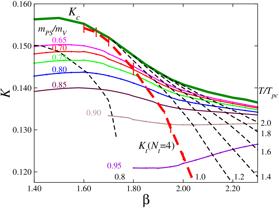1, corresponding to $m_{\rm PS}/m_{\rm V}=0.65$ , 0.70, 0.75, 0.80, 0.85, 0.90 and 0.95.

Refer to caption — Figure 1: Lines of constant physics (LCP) determined by $m_{\rm PS}/m_{\rm V}$ at $T=0$ (solid lines) for $m_{\rm PS}/m_{\rm V}=0.65$ , 0.70, 0.75, 0.80, 0.85, 0.90 and 0.95. $K_{c}$ is the chiral limit, i.e. $m_{\rm PS}/m_{\rm V}=0$ . Dashed lines represent lines of constant $T/T_{pc}$ on $N_{t}=4$ lattices, where $T_{pc}$ is the pseudo-critical temperature corresponding to $K_{t}(N_{t}=4)$ shown by the thick dashed line.

The temperature $T$ is estimated by the zero-temperature vector meson mass $m_{\rm V}a(\beta,K)$ using

\displaystyle\frac{T}{m_{\rm V}}(\beta,K)=\frac{1}{N_{t}\times m_{\rm V}a(\beta,K)}.

(5)

The lines of constant $T/T_{pc}$ is determined by the ratio of ${T}/{m_{\rm V}}$ to ${T_{pc}}/{m_{\rm V}}$ where $T_{pc}/m_{\rm V}$ is obtained by $T/m_{\rm V}$ at $K_{t}$ on the same LCP. We use an interpolation function, $T_{pc}/m_{\rm V}=A(1+B(m_{\rm PS}/m_{\rm V})^{2})/(1+C(m_{\rm PS}/m_{\rm V})^{2})$ with $A=0.2253(71)$ , $B=-0.933(17)$ and $C=-0.820(39)$ , obtained in Ref. [8] to evaluate $T_{pc}/m_{\rm V}$ for each $m_{\rm PS}/m_{\rm V}$ . The bold dashed line denoted as $K_{t}(N_{t}=4)$ in Fig. 1 represents the pseudo-critical line $T/T_{pc}=1$ . The thin dashed lines represent the results for $T/T_{pc}=0.8$ , 1.2, 1.4, 1.6, 1.8, 2.0 at $N_{t}=4$ .

We perform finite temperature simulations on a lattice with a temporal extent $N_{t}=4$ and a spatial extent $N_{s}=16$ along the LCP’s at $m_{\rm PS}/m_{\rm V}=0.65$ and 0.80. The standard hybrid Monte Carlo algorithm is employed to generate full QCD configurations with two flavors of dynamical quarks. The length of one trajectory is unity and the step size of the molecular dynamics is tuned to achieve an acceptance rate greater than 70%. Runs are carried out in the range $\beta=1.50$ –2.40 at thirteen values of $T/T_{pc}\sim 0.82$ –4.0 for $m_{\rm PS}/m_{\rm V}=0.65$ and twelve values of $T/T_{pc}\sim 0.76$ –3.0 for $m_{\rm PS}/m_{\rm V}=0.80$ . Our simulation parameters and the corresponding temperatures are summarized in Table 1. Because the determination of the pseudo critical line is more difficult than the calculation of $T/m_{\rm V}$ , the dominant source for the error of $T/T_{pc}$ in Table 1 is the overall factor $T_{pc}/m_{\rm V}$ . The number of trajectories for each run after thermalization is 5000–6000. We measure physical quantities at every 10 trajectories. The study of heavy quark free energies at $\mu_{q}=0$ using the same configurations have been already published in Ref. [24].

Table 1: Simulation parameters for

m_{\rm PS}/m_{\rm V}=0.65

(left) and

m_{\rm PS}/m_{\rm V}=0.80

(right) on a

16^{3}\times 4

lattice.

$\beta$	$K$	$T/T_{pc}$	Traj.	$\beta$	$K$	$T/T_{pc}$	Traj.
$1.50$	$0.150290$	$0.82(3)$	$5000$	$1.50$	$0.143480$	$0.76(4)$	$5500$
$1.60$	$0.150030$	$0.86(3)$	$5000$	$1.60$	$0.143749$	$0.80(4)$	$6000$
$1.70$	$0.148086$	$0.94(3)$	$5000$	$1.70$	$0.142871$	$0.84(4)$	$6000$
$1.75$	$0.146763$	$1.00(4)$	$5000$	$1.80$	$0.141139$	$0.93(5)$	$6000$
$1.80$	$0.145127$	$1.07(4)$	$5000$	$1.85$	$0.140070$	$0.99(5)$	$6000$
$1.85$	$0.143502$	$1.18(4)$	$5000$	$1.90$	$0.138817$	$1.08(5)$	$6000$
$1.90$	$0.141849$	$1.32(5)$	$5000$	$1.95$	$0.137716$	$1.20(6)$	$6000$
$1.95$	$0.140472$	$1.48(5)$	$5000$	$2.00$	$0.136931$	$1.35(7)$	$5000$
$2.00$	$0.139411$	$1.67(6)$	$5000$	$2.10$	$0.135860$	$1.69(8)$	$5000$
$2.10$	$0.137833$	$2.09(7)$	$5000$	$2.20$	$0.135010$	$2.07(10)$	$5000$
$2.20$	$0.136596$	$2.59(9)$	$5000$	$2.30$	$0.134194$	$2.51(13)$	$5000$
$2.30$	$0.135492$	$3.22(12)$	$5000$	$2.40$	$0.133395$	$3.01(15)$	$5000$
$2.40$	$0.134453$	$4.02(15)$	$5000$

II.2 Critical temperature

Table 2: Finite temperature transition/crossover point

K_{t}

for

N_{t}=4

and

6

. Results for

m_{\rm PS}(T=0)/m_{\rm V}(T=0)

m_{\rm PS}a(T=0)

m_{q}^{\rm AWI}a(T>0)

T_{pc}/m_{\rm V}(T=0)

T_{pc}/\sqrt{\sigma}

T_{pc}r_{0}

, and

m_{\rm PS}r_{0}

, are interpolated to the

K_{t}

line,

$\beta$	$K_{t}$	$K_{c}$	$m_{\rm PS}/m_{\rm V}$	$m_{\rm PS}a$	$m_{q}^{\rm AWI}a$	$T_{pc}/m_{\rm V}$	$T_{pc}/\sqrt{\sigma}$	$T_{pc}r_{0}$	$m_{\rm PS}r_{0}$
$N_{t}=4$
1.700	0.15014(33)	0.151987(22)	0.509(35)	0.579(51)		0.2197(47)
1.800	0.14425(16)	0.147678(15)	0.7070(79)	0.849(18)	0.1107(77)	0.2083(21)	0.4204(29)	0.4716(42)	1.601(37)
1.850	0.14019(18)	0.145526(58)	0.7905(60)	1.031(15)	0.1864(72)	0.1917(20)	0.4359(60)	0.484(11)	1.994(55)
1.900	0.13621(15)	0.143737(48)	0.8525(39)	1.183(11)	0.2464(49)	0.1801(12)	0.4382(70)	0.484(16)	2.290(79)
1.925	0.13417(23)				0.2725(67)
1.950	0.13040(97)	0.142072(14)	0.9051(64)	1.440(66)	0.363(25)	0.1572(62)
2.000	0.12371(73)	0.140811(55)	0.9450(36)	1.689(39)	0.500(18)	0.1398(29)
2.100	0.10921(43)	0.139020(21)	0.9790(13)	2.196(18)		0.1114(9)
$N_{t}=6$
1.950	0.14090(13)	0.142072(14)	0.591(21)	0.448(24)	0.0451(51)	0.2202(44)	0.4336(40)	0.4973(58)	1.336(73)
2.000	0.13861(21)	0.140811(55)	0.725(16)	0.580(27)	0.080(10)	0.2086(53)	0.4639(77)	0.530(13)	1.842(98)
2.100	0.13365(40)	0.139020(21)	0.8635(78)	0.821(34)	0.175(13)	0.1753(58)	0.491(12)	0.570(13)	2.81(13)
2.200	0.12539(25)	0.137658(53)	0.9481(19)	1.240(16)	0.3607(67)	0.1275(15)
2.300	0.11963(15)	0.136513(85)	0.9724(12)	1.454(8)	0.4813(39)	0.1114(6)

Table 3: The critical point

(\beta_{ct})

and critical temperature

(T_{c})

in the chiral limit obtained by various fitting procedures. The fit range for

\beta

is written in “

\beta

range”.

T_{c}

in a physical unit is estimated from the vector meson mass

m_{\rm V}=m_{\rho}=770{\rm MeV}

$N_{t}$	$h\sim m_{q}a$	$\beta$ range	$\beta_{ct}$	$T_{c}$ ( $m_{\rm V}$ -input)	$T_{c}r_{0}$
4	$1/K_{t}-1/K_{c}$	1.70–1.95	1.619(10)	180(3) MeV
4	$1/K_{t}-1/K_{c}$	1.70–1.90	1.611(12)	179(3) MeV
4	$(m_{\rm PS}a)^{2}$	1.70–1.95	1.559(16)	172(3) MeV
4	$(m_{\rm PS}a)^{2}$	1.70–1.90	1.552(16)	171(3) MeV
4	$m_{q}^{\rm AWI}a$	1.80–1.90	1.601(20)	177(4) MeV
4	$m_{q}^{\rm AWI}a$	1.80–1.95	1.596(18)	176(3) MeV
6	$1/K_{t}-1/K_{c}$	1.95–2.20	1.870(6)	184(5) MeV	0.434(9)
6	$1/K_{t}-1/K_{c}$	1.95–2.10	1.840(14)	171(4) MeV	0.401(16)
6	$(m_{\rm PS}a)^{2}$	1.95–2.20	1.835(9)	170(4) MeV	0.396(12)
6	$(m_{\rm PS}a)^{2}$	1.95–2.10	1.786(25)	160(9) MeV	0.350(23)
6	$m_{q}^{\rm AWI}a$	1.95–2.20	1.835(10)	170(4) MeV	0.396(12)
6	$m_{q}^{\rm AWI}a$	1.95–2.10	1.810(19)	167(4) MeV	0.372(20)

We update the analysis of the pseudo critical temperature done in Refs. [7, 8], performing additional simulations at $\beta=6/g^{2}=1.7$ and $1.8$ on an $N_{s}^{3}\times N_{t}=16\times 4$ lattice and at $1.9$ and $1.95$ on $N_{s}^{3}\times N_{t}=16^{3}\times 6$ . The number of trajectories for each new run is 1050–4200 after thermalization. We add the new data to the data in Refs. [7, 8] and determine the pseudo-critical hopping parameters $K_{t}$ defined from the peak of the Polyakov loop susceptibility on $16^{3}\times 4$ and $16^{3}\times 6$ lattices, as a function of $\beta$ . Figures 2 and 3 are the results of the Polyakov loop $\langle L\rangle$ and Polyakov loop susceptibility $\chi_{L}$ , respectively. We find a pronounced peak in the Polyakov loop susceptibility except for $\beta=1.90$ at $N_{t}=6$ . The peak position of the susceptibility $(K_{t})$ is determined by fitting three or four data near the peak with the Gaussian form. The results are summarized in Table 2 together with values of some quantities at $K_{t}$ to set a physical scale.

We use the data of the pseudo-scalar and vector meson masses at $T=0$ , $m_{\rm PS}$ and $m_{\rm V}$ , summarized in the Table IV of Ref. [8], and interpolate them following the method discussed in Refs. [7] and [8]. We also calculate the current quark mass defined through an axial vector Ward-Takahashi identity, $\nabla_{\mu}A_{\mu}=2m_{q}^{\rm AWI}P+O(a),$ where $P$ is the pseudo-scalar density and $A_{\mu}$ the $\mu$ -th component of the local axial vector current [28, 29]. Because the $T$ -dependence in $m_{q}^{\rm AWI}$ is small, we use the data of $m_{q}^{\rm AWI}$ obtained in finite temperature simulations at $N_{t}=4$ and $6$ [7, 8] . In Table 2, $m_{q}^{\rm AWI}$ on the $K_{t}$ line are obtained using a cubic spline interpolation for each $\beta$ . A straight line interpolation leads to almost identical results within statistical errors. The values of the string tension $\sigma$ and the Sommer scale $r_{0}$ [30] are estimated by interpolating or extrapolating the data at $\beta=1.80,1.95,2.10$ and $2.20$ [11] in the $(\beta,1/K-1/K_{c})$ parameter plane.

The results of the pseudo-critical temperature are also shown in Table 2. We plot $T_{pc}/m_{\rm V}$ as a function of $(m_{\rm PS}/m_{\rm V})^{2}$ in Fig. 4, and find that the results of $N_{t}=4$ and 6 agree with each other. Note that $T_{pc}/m_{\rm V}$ vanishes in the heavy quark limit $m_{\rm PS}/m_{\rm V}=1$ . Figure 4 suggests $T_{pc}/m_{\rm V}\sim 0.22$ ( $T_{pc}\sim 170{\rm MeV}$ ) in the chiral limit.

We denote the critical temperature in the chiral limit as $T_{c}$ . As discussed in [7, 9], the subtracted chiral condensate [29] satisfies the scaling behavior with the critical exponents and scaling function of the 3-dimensional O(4) spin model. For the reduced temperature $t$ and external magnetic field $h$ , we adopt $t\sim\beta-\beta_{ct}$ and $h\sim m_{q}$ , where $\beta_{ct}$ is the critical transition point in the chiral limit. For a precise determination of $T_{c}$ , we need to deduce $\beta_{ct}$ from the data. In this study, we perform critical scaling fits assuming that the pseudo-critical temperature $t_{pc}$ from the Polyakov loop susceptibility, as well as that from the chiral condensate, follows the scaling law $t_{pc}\sim h^{1/y}$ with the O(4) critical exponent $1/y\equiv 1/(\beta\delta)=0.537(7)$ . In practice, we fit the data of $\beta_{pc}(K)$ , i.e. the inverse function of $K_{t}(\beta)$ in Table 2, by

\displaystyle\beta_{pc}=\beta_{ct}+Ah^{1/y}

(6)

with two free parameters, $\beta_{ct}$ and $A$ .

For the quark mass $m_{q}\sim h$ in the scaling fits, we test three variants. The first is $m_{q}a\sim 1/K-1/K_{c}$ , where $K_{c}$ is the chiral point at which the pion mass vanishes at $T=0$ for each $\beta$ . The second is $m_{q}a\sim(m_{\rm PS}a)^{2}$ . The third is $m_{q}^{\rm AWI}a$ , i.e. the quark mass defined by the axial vector Ward-Takahashi identity. We plot $\beta_{pc}$ as a function of $1/K-1/K_{c}$ (left), $(m_{\rm PS}a)^{2}$ (center) and $m_{q}^{\rm AWI}a$ (right) in Fig. 5. The results of $\beta_{ct}$ and $T_{c}$ are summarized in Table 3, where $T_{c}$ in MeV is calculated by $T_{c}=1/[N_{t}a(\beta_{ct})]$ with $a$ from the vector meson mass $m_{\rm V}(T=0)=m_{\rho}=770$ MeV at $\beta_{ct}$ on $K_{c}$ . We test two fit ranges of $\beta$ for each extrapolation, which is denoted in Table 3 as “ $\beta$ range”. We note that these O(4) fits reproduce the data of $\beta_{pc}$ much better than a naive linear fit $\beta_{pc}=\beta_{ct}+Ah$ . A tentative conclusion is that the critical temperature in the chiral limit is in the range 171–180 MeV for $N_{t}=4$ and 160–184 MeV for $N_{t}=6$ . There is still a large uncertainty from the choice of the fit ansatz and the fit range. To remove this, further simulations at lighter quark masses are necessary.

For a comparison with other groups, we estimate $T_{c}$ in units of the Sommer scale $r_{0}$ [30] at $\beta_{ct}$ in the chiral limit for $N_{t}=6$ . Using the data of $r_{0}/a$ in the chiral limit at $\beta=1.80$ , 1.95 and 2.10 [11], we interpolate $a/r_{0}$ by a quadratic function and calculate $T_{c}r_{0}=(N_{t}a/r_{0})^{-1}$ . The estimates are about $T_{c}r_{0}\approx 0.40$ , as listed in Table 3. These values are close to $T_{c}r_{0}=0.402(29)$ obtained by the MILC Collaboration using the asqtad quark action in 2+1 flavor QCD [31] ¹¹ 1 Originally, $T_{c}$ is given in units of $r_{1}$ in Ref. [31]. The scale of $T_{c}$ has been converted to $r_{0}$ using $r_{0}/r_{1}=1.4795$ [32].. On the other hand, the RBC-Bielefeld Collaboration obtained $T_{c}r_{0}=0.444(6)^{+12}_{-3}$ using a 2+1 flavor p4fat3 improved staggered quark action [32]. From a simulation of 2 flavor QCD using a clover improved Wilson action and the standard one-plaquette gauge action, the DIK Collaboration obtained $T_{c}r_{0}=0.438(6)^{+13}_{-7}$ at the physical pion mass point, and the value in the chiral limit is $2\%$ smaller than this value [33]. Our result is somewhat smaller than these values. Finally, the Budapest-Wuppertal group used a stout-link improved staggered fermion action and fixed the scale by the pion decay constant $f_{\pi}$ . They found that $T_{c}$ determined by the chiral susceptibility is $T_{c}=151(3)(3)$ MeV and that by the renormalized Polyakov loop is $T_{c}=176(3)(4)$ MeV in the continuum limit at the physical point [34]. Our result is close to their result defined by the Polyakov loop. For further discussions, see Refs. [35, 36, 37].

III Equation of state at finite densities by the Taylor expansion method

The main difficulty in a study of QCD at finite density is that the Boltzmann weight is complex for nonzero $\mu_{q}$ . The quark matrix at zero density have the $\gamma_{5}$ Hermiticity $M^{\dagger}=\gamma_{5}M\gamma_{5}$ which guarantees that the quark determinant is real. However, at $\mu_{q}\neq 0$ , we have only

\displaystyle M^{\dagger}(\mu_{q})=\gamma_{5}M(-\mu_{q})\gamma_{5},

(7)

from Eq. (4). Therefore, the quark determinant is complex for $\mu_{q}\neq 0$ .

Because configurations cannot be generated with a complex probability, the conventional Monte Carlo method is not applicable at $\mu_{q}\neq 0$ . At present, there are three methods to study finite density QCD, all of which are applicable for small $\mu_{q}$ regions. The simplest is the method based on a Taylor expansion in terms of $\mu_{q}/T$ around $\mu_{q}=0$ [22, 17, 38, 39]. Because the simulations at $\mu_{q}=0$ is free from the complex weight problem, the expansion coefficients, i.e. derivatives of physical quantities with respect to $\mu_{q}/T$ , can be evaluated by a conventional Monte Carlo simulation. The second approach is the reweighting method [40, 41, 42, 43]. Performing simulations at $\mu_{q}=0$ , expectation values at finite $\mu_{q}$ are computed adopting a corrected Boltzmann weight. For the correction, quark determinant at finite $\mu_{q}$ is estimated numerically. Because fluctuations in the complex phase of the determinant are large at large $\mu_{q}$ and/or large lattice volume, a reliable calculation of expectation value becomes gradually difficult off the small $\mu_{q}$ and small lattice volume region due to the sign problem [44, 45]. The third approach is the analytic continuation from simulations with imaginary chemical potentials [46, 47]. Since the equation (7) is generalized to $M^{\dagger}(\mu_{q})=\gamma_{5}M(-\mu_{q}^{*})\gamma_{5}$ for complex $\mu_{q}$ , the Boltzmann weight is real and simulations are possible when the chemical potential is purely imaginary. Using results by the imaginary chemical potential simulations, information at a real chemical potential can be obtained by an analytic continuation. The analytic continuation is usually based on a Taylor expansion in terms of $\mu_{q}$ around $\mu_{q}=0$ for the study in the low density region, and improvements of the analytic continuation have been also discussed in [48, 49, 50] to obtain reliable results in a wide range of real $\mu_{q}$ .

In this section, we adopt the Taylor expansion method to study the effects of $\mu_{q}$ in the equation of state. Most of thermodynamic quantities, such as energy density, quark number, order parameters and various susceptibilities, are given by derivatives of the thermodynamic grand canonical potential $\omega/T^{4}\equiv-(\ln{\cal Z})/(VT^{3})$ . Also, pressure, which is given by $\omega$ itself, is evaluated by integrating a derivative of $\omega$ in current studies of the equation of state. Therefore, the calculations of the derivative of $\omega$ is basic for the study of QCD thermodynamics by lattice simulations, and the Taylor expansion method calculating higher order derivatives in $\mu_{q}$ is the most natural extension from the study at $\mu_{q}=0$ to finite $\mu_{q}$ .

III.1 Taylor expansion of the grand canonical potential

We study pressure $p$ and quark number densities $n_{u}$ and $n_{d}$ defined by derivatives of the partition function ${\cal Z}(T,\mu_{u},\mu_{d})$ :

\displaystyle\frac{p}{T^{4}}=\frac{1}{VT^{3}}\ln{\cal Z}\equiv-\frac{\omega}{T^{4}},\hskip 22.76219pt\frac{n_{f}}{T^{3}}=\frac{1}{VT^{3}}\frac{\partial\ln{\cal Z}}{\partial(\mu_{f}/T)}=\frac{\partial(p/T^{4})}{\partial(\mu_{f}/T)},\hskip 14.22636pt(f=u,\,d)

(8)

where $\mu_{u}$ and $\mu_{d}$ are the chemical potentials for the u and d quarks. Let us define the quark chemical potential $\mu_{q}=(\mu_{u}+\mu_{d})/2$ and the isospin chemical potential $\mu_{I}=(\mu_{u}-\mu_{d})/2$ . Taylor expansion coefficients of physical quantities are given by derivatives of them in terms of $\mu_{u}$ and $\mu_{d}$ , or equivalently $\mu_{q}$ and $\mu_{I}$ . We evaluate these coefficients at $\mu_{u}=\mu_{d}=0$ and study the physical quantities as functions of $T$ and $\mu_{q}$ in the isosymmetric case $\mu_{u}=\mu_{d}=\mu_{q}$ (i.e. $\mu_{I}=0$ ).

We define the susceptibility of quark number by

\displaystyle\frac{\chi_{q}}{T^{2}}=\left(\frac{\partial}{\partial(\mu_{u}/T)}+\frac{\partial}{\partial(\mu_{d}/T)}\right)\frac{n_{u}+n_{d}}{T^{3}},

(9)

and the susceptibility of isospin number by

\displaystyle\frac{\chi_{I}}{T^{2}}=\left(\frac{\partial}{\partial(\mu_{u}/T)}-\frac{\partial}{\partial(\mu_{d}/T)}\right)\frac{n_{u}-n_{d}}{T^{3}}.

(10)

These susceptibilities correspond to the fluctuations of baryon number and isospin number in the medium, respectively [53]. They are expected to behave quite differently near the critical point in the $(T,\mu_{q})$ plane.

We define the Taylor expansion coefficients of the pressure $p(T,\mu_{q})$ for the case $\mu_{u}=\mu_{d}=\mu_{q}$ as

\frac{p}{T^{4}}=\sum_{n=0}^{\infty}c_{n}(T)\left(\frac{\mu_{q}}{T}\right)^{n},\hskip 22.76219ptc_{n}(T)=\frac{1}{n!}\frac{N_{t}^{3}}{N_{s}^{3}}\left.\frac{\partial^{n}\ln{\cal Z}}{\partial(\mu_{q}/T)^{n}}\right|_{\mu_{q}=0}.

(11)

Here, $c_{0}(T)$ is the pressure at $\mu_{q}=0$ and has been computed by the CP-PACS Collaboration with the same action on $16^{3}\times 4$ and $16^{3}\times 6$ lattices [7, 8]. Its value in the quenched limit is given in [51].

We also expand the quark number and isospin susceptibilities for the case $\mu_{u}=\mu_{d}=\mu_{q}$ :

\displaystyle\frac{\chi_{q}(T,\mu_{q})}{T^{2}}=2c_{2}+12c_{4}\left(\frac{\mu_{q}}{T}\right)^{2}+\cdots,\hskip 14.22636pt\frac{\chi_{I}(T,\mu_{q})}{T^{2}}=2c^{I}_{2}+12c^{I}_{4}\left(\frac{\mu_{q}}{T}\right)^{2}+\cdots,

(12)

where

c^{I}_{n}=\left.\frac{1}{n!}\frac{N_{t}^{3}}{N_{s}^{3}}\frac{\partial^{n}\ln{\cal Z}(T,\mu_{q}+\mu_{I},\mu_{q}-\mu_{I})}{\partial(\mu_{I}/T)^{2}\partial(\mu_{q}/T)^{n-2}}\right|_{\mu_{q}=0,\mu_{I}=0},

(13)

III.1.1 Free quark-gluon gas at high temperature

We expect QCD in the high temperature limit is described as free gas of quark and gluon. The pressure of the free gas in the continuum theory is given by

\displaystyle\frac{p}{T^{4}}=\frac{8\pi^{2}}{45}+\sum_{f=u,d}\left[\frac{7\pi^{2}}{60}+\frac{1}{2}\left(\frac{\mu_{f}}{T}\right)^{2}+\frac{1}{4\pi^{2}}\left(\frac{\mu_{f}}{T}\right)^{4}\right].

(14)

Note that the $\mu_{q}$ -dependence appears only through terms of $\mu_{q}^{2}$ and $\mu_{q}^{4}$ . The quark number density is a cubic function of $\mu_{q}$ too. The quark number and isospin susceptibilities are the same for the free quark-gluon gas and are given by a quadratic function

\displaystyle\frac{\chi_{q}}{T^{2}}=\frac{\chi_{I}}{T^{2}}=N_{\rm f}\left[1+\frac{3}{\pi^{2}}\left(\frac{\mu_{q}}{T}\right)^{2}\right].

(15)

Therefore, the Taylor expansion will converge well in the high temperature region.

III.1.2 Hadron resonace gas at low temperature

On the other hand, QCD at low temperature may be modeled by free gas of hadron resonances [52]. The partition function of the hadron resonance gas consists of mesonic and baryonic contributions,

\displaystyle\ln{\cal Z}(T,V,\mu_{q})=\sum_{i\in\;{\rm mesons}}\hskip-8.53581pt\ln{\cal Z}^{M}_{m_{i}}(T,V,\mu_{q})+\hskip-8.53581pt\sum_{i\in\;{\rm baryons}}\hskip-8.53581pt\ln{\cal Z}^{B}_{m_{i}}(T,V,\mu_{q})\;,

(16)

where

\ln{\cal Z}^{M/B}_{m_{i}}(T,V,\mu_{q})=\mp\frac{V}{2\pi^{2}}\int_{0}^{\infty}dkk^{2}\ln(1\mp z_{i}e^{-\varepsilon_{i}/T})\quad,

(17)

with energies $\varepsilon_{i}^{2}=k^{2}+m_{i}^{2}$ and fugacities

z_{i}=\exp\left((3B_{i}\mu_{q})/T\right)\quad.

(18)

Here $B_{i}$ is the baryon number: $B_{i}=1,-1$ and $0$ for baryons, anti-baryons and mesons, respectively. The upper sign in Eq. (17) is for bosons, while the lower sign for fermions. Note that ${\cal Z}^{M}_{m_{i}}$ is actually independent of $\mu_{q}$ . Expanding the logarithms in powers of fugacity, the integration over momenta, $k$ , can be carried out:

\ln{\cal Z}^{M/B}_{m_{i}}=\frac{VTm_{i}^{2}}{2\pi^{2}}\sum_{l=1}^{\infty}\left\{\begin{array}[]{c}1\\ (-1)^{l+1}\end{array}\right\}l^{-2}K_{2}\left(\frac{lm_{i}}{T}\right)z_{i}^{l}\quad,

(19)

where $K_{2}$ is a modified Bessel function. For $m_{i}\gg T$ , the Bessel function can be approximated by $K_{2}(x)\sim\sqrt{\pi/2x}\;{\rm e}^{-x}(1+15/8x+{\cal O}(x^{-2}))$ . Terms with $\ell\geq 2$ in the series given in Eq. (19) thus are exponentially suppressed.

Let us study the $\mu_{q}$ -dependence of the partition function. The mesonic sector has no $\mu_{q}$ -dependence because $B_{i}=0$ for mesons. On the other hand, the baryonic sector can be approximated by the leading term in the expansion of $z_{i}$ , since all baryons are heavier than a typical temperature scale. We obtain

\frac{p(T,\mu_{q})}{T^{4}}-\frac{p(T,0)}{T^{4}}=\frac{1}{VT^{3}}\left[\ln{\cal Z}(T,\mu_{q})-\ln{\cal Z}(T,0)\right]\simeq F(T)\left[\cosh\left(\frac{3\mu_{q}}{T}\right)-1\right],

(20)

with

\displaystyle F(T)=\frac{1}{\pi^{2}}\sum_{i\in\;{\rm baryons}}\left(\frac{m_{i}}{T}\right)^{2}K_{2}\left(\frac{m_{i}}{T}\right).

(21)

Note that each term in the sum for $F$ now counts both baryons and anti-baryons. The quark number susceptibility is then given by

\frac{\chi_{q}}{T^{2}}=9F(T)\cosh\left(\frac{3\mu_{q}}{T}\right).

(22)

From Eq. (20), the ratios of the expansion coefficients of $p/T^{4}$ in $\mu_{q}/T$ are derived,

\frac{c_{2n+2}}{c_{2n}}=\frac{9}{(2n+2)(2n+1)}.

(23)

The ratio decreases as the order becomes higher. This means that the contribution from the higher order terms of $\mu_{q}/T$ is small in the region of $\mu_{q}/T\mathrel{\hbox to0.0pt{\raise 2.20013pt\hbox{$<$}\hss}{\lower 2.20013pt\hbox{$\sim$}}}O(1)$ .

III.1.3 Numerical study near the transition temperature

The behavior near the transition temperature is non-trivial. We expect a critical point at finite $\mu_{q}$ . The Taylor expansion must break down at that point. We perform numerical simulations to study the expansion coefficients near the transition point. Using $\mu\equiv\mu_{q}a$ , the explicit forms of the Taylor expansion coefficients are

\displaystyle\hskip-36.98857ptc_{2}=\frac{N_{t}}{2N_{s}^{3}}{\cal A}_{2},\hskip 8.53581ptc_{4}=\frac{1}{4!N_{s}^{3}N_{t}}({\cal A}_{4}-3{\cal A}_{2}^{2}),\hskip 8.53581ptc_{2}^{I}=\frac{N_{t}}{2N_{s}^{3}}{\cal B}_{2},\hskip 8.53581ptc_{4}^{I}=\frac{1}{4!N_{s}^{3}N_{t}}({\cal B}_{4}-{\cal B}_{2}{\cal A}_{2}),

(24)

	$\displaystyle{\cal A}_{2}$	$\displaystyle=$	$\displaystyle\left\langle{\cal D}_{2}\right\rangle+\left\langle{\cal D}_{1}^{2}\right\rangle,\hskip 14.22636pt{\cal A}_{4}=\left\langle{\cal D}_{4}\right\rangle+4\left\langle{\cal D}_{3}{\cal D}_{1}\right\rangle+3\left\langle{\cal D}_{2}^{2}\right\rangle+6\left\langle{\cal D}_{2}{\cal D}_{1}^{2}\right\rangle+\left\langle{\cal D}_{1}^{4}\right\rangle,$
	$\displaystyle{\cal B}_{2}$	$\displaystyle=$	$\displaystyle\left\langle{\cal D}_{2}\right\rangle,\hskip 14.22636pt{\cal B}_{4}=\left\langle{\cal D}_{4}\right\rangle+2\left\langle{\cal D}_{3}{\cal D}_{1}\right\rangle+\left\langle{\cal D}_{2}^{2}\right\rangle+\left\langle{\cal D}_{2}{\cal D}_{1}^{2}\right\rangle,$		(25)

with

\displaystyle{\cal D}_{n}=N_{f}\frac{\partial^{n}\ln\det M}{\partial\mu^{n}},

(26)

i.e.,

$\displaystyle{\cal D}_{1}$	$\displaystyle=$	$\displaystyle N_{f}{\rm tr}\left(M^{-1}\frac{\partial M}{\partial\mu}\right),\hskip 28.45274pt{\cal D}_{2}\ =\ N_{f}\left[{\rm tr}\left(M^{-1}\frac{\partial^{2}M}{\partial\mu^{2}}\right)-{\rm tr}\left(M^{-1}\frac{\partial M}{\partial\mu}M^{-1}\frac{\partial M}{\partial\mu}\right)\right],$
$\displaystyle{\cal D}_{3}$	$\displaystyle=$	$\displaystyle N_{f}\left[{\rm tr}\left(M^{-1}\frac{\partial^{3}M}{\partial\mu^{3}}\right)-3{\rm tr}\left(M^{-1}\frac{\partial M}{\partial\mu}M^{-1}\frac{\partial^{2}M}{\partial\mu^{2}}\right)+2{\rm tr}\left(M^{-1}\frac{\partial M}{\partial\mu}M^{-1}\frac{\partial M}{\partial\mu}M^{-1}\frac{\partial M}{\partial\mu}\right)\right],$
$\displaystyle{\cal D}_{4}$	$\displaystyle=$	$\displaystyle N_{f}\left[{\rm tr}\left(M^{-1}\frac{\partial^{4}M}{\partial\mu^{4}}\right)-4{\rm tr}\left(M^{-1}\frac{\partial M}{\partial\mu}M^{-1}\frac{\partial^{3}M}{\partial\mu^{3}}\right)-3{\rm tr}\left(M^{-1}\frac{\partial^{2}M}{\partial\mu^{2}}M^{-1}\frac{\partial^{2}M}{\partial\mu^{2}}\right)\right.$	(27)
		$\displaystyle\left.+12{\rm tr}\left(M^{-1}\frac{\partial M}{\partial\mu}M^{-1}\frac{\partial M}{\partial\mu}M^{-1}\frac{\partial^{2}M}{\partial\mu^{2}}\right)-6{\rm tr}\left(M^{-1}\frac{\partial M}{\partial\mu}M^{-1}\frac{\partial M}{\partial\mu}M^{-1}\frac{\partial M}{\partial\mu}M^{-1}\frac{\partial M}{\partial\mu}\right)\right].$	(27)

The derivative of the fermion matrix $M$ at $\mu=0$ is

\displaystyle\left(\frac{\partial^{n}M}{\partial\mu^{n}}\right)_{x,y}=\left\{\begin{array}[]{l}-K\left((1-\gamma_{4})U_{4}(x)~\delta_{x+\hat{4},y}-(1+\gamma_{4}){U_{4}}^{\dagger}(x-\hat{4})~\delta_{x-\hat{4},y}\right)\ \ {\rm for}\ n:{\rm odd.}\\ -K\left((1-\gamma_{4})U_{4}(x)~\delta_{x+\hat{4},y}+(1+\gamma_{4}){U_{4}}^{\dagger}(x-\hat{4})~\delta_{x-\hat{4},y}\right)\ \ {\rm for}\ n:{\rm even.}\end{array}\right.

III.2 Random noise method

We apply a random noise method to evaluate the traces in Eq. (27). As we will see later, this method is effective when off-diagonal elements of the matrix are small. Therefore, the method works well for traces over spatial indices: Because the inverse of the quark matrix $M^{-1}(x,y)$ decreases as a function of $|x-y|$ , the off-diagonal elements in the spatial coordinate will be smaller than the diagonal ones. The random noise method will work well to suppress these small contaminations of off-diagonal elements. On the other hand, the off-diagonal elements in the color and spinor indices at the same spatial point are not suppressed by $|x-y|$ , and will have the same magnitude as the diagonal elements. Because a staggered-type quark does not have the spinor index at a spatial point, the number of off-diagonal elements is only 6 in the $3\times 3$ matrix, the contamination of off-diagonal elements may be not so serious. However, for Wilson-type quarks, because the number of color-spinor index is $3\times 4$ , the number of the off-diagonal elements in the quark matrix is 11 times larger than the diagonal one, so that the color-spinor index should be treated more carefully with Wilson-type quarks. In this study, we apply the random noise method for the spatial coordinates only, repeating the calculation for each of the color and spinor indices.

We generate noise vectors $\left(\eta_{i,\alpha}\right)_{x,\beta}\equiv\eta(i,x)\,\delta_{\alpha,\beta}$ , which satisfy

\displaystyle\frac{1}{N_{\rm noise}}\sum_{i=1}^{N_{\rm noise}}\eta(i,x)\eta^{*}(i,y)\approx\delta_{x,y}

(31)

for large $N_{\rm noise}$ . We adopt U(1) random numbers as $\eta$ , which are complex random numbers with $|\eta|=1$ and are generated from uniform random numbers $\theta\in[0,2\pi)$ with $\eta=e^{i\theta}$ . For each color-spinor index ( $\alpha=1,\cdots,12$ ), we generate $N_{\rm noise}$ noise vectors ( $i=1\sim N_{\rm noise}$ ). Then $\lim_{N_{\rm noise}\to\infty}(1/N_{\rm noise})\sum_{i=1}^{N_{\rm noise}}\sum_{\alpha=1}^{12}\left(\eta_{i,\alpha}\right)_{x,\beta}\left(\eta_{i,\alpha}^{*}\right)_{y,\gamma}=\delta_{x,y}\delta_{\beta,\gamma}$ , hence

\displaystyle{\rm tr}\left(\frac{\partial^{n_{1}}M}{\partial\mu^{n_{1}}}M^{-1}\frac{\partial^{n_{2}}M}{\partial\mu^{n_{2}}}\cdots M^{-1}\right)

\displaystyle\approx

\displaystyle\frac{1}{N_{\rm noise}}\sum_{i=1}^{N_{\rm noise}}\sum_{\alpha=1}^{12}\eta_{i,\alpha}^{\dagger}\frac{\partial^{n_{1}}M}{\partial\mu^{n_{1}}}X_{i,\alpha},\hskip 28.45274pt(n=1,2,\cdots),

(32)

where $X_{i,\alpha}=M^{-1}(\partial^{n_{2}}M/\partial\mu^{n_{2}})\cdots M^{-1}\eta_{i,\alpha}$ . To obtain $X$ , we solve equations $MX_{n}=Y_{n}$ recursively with $Y_{1}=\eta$ , $Y_{2}=(\partial^{n}M/\partial\mu^{n})M^{-1}\eta=(\partial^{n}M/\partial\mu^{n})X_{1}$ , etc.

Because $N_{\rm noise}^{-1}\sum_{i}\eta(i,x)\eta^{*}(i,y)$ is $O(\sqrt{1/N_{\rm noise}}\,)$ for $x\neq y$ , errors due to finite $N_{\rm noise}$ decrease as $O(\sqrt{1/N_{\rm noise}}\,)$ . However, these errors are produced from all off-diagonal elements of the matrix in Eq. (32), hence these are proportional to the magnitude and number of the off-diagonal elements. Therefore, when the off-diagonal elements are not smaller than the diagonal elements, a number of noise vectors are needed to remove the error. This is the reason why we do not use the random noise method for the color-spinor index.

For a product of traces, the random noise vectors for each trace must be independent. We compute such product by subtracting the contribution of the same noise vector from the naive product of two noise averages for each trace. This effectively increases the number of noises to $N_{\rm noise}(N_{\rm noise}-1)$ for the products and thus suppresses their errors due to the noise method.

We then average over configurations to evaluate the expectation values in Eq. (25). In addition to the errors due to the noise method, the statistical fluctuation of configurations contributes to the final error. To check the relative amount of the errors from the noise method, we calculate the operators ${\cal D}_{n}$ ( $n=1$ -4) using two independent sets of noise vectors with $N_{\rm noise}=10$ on the same configurations. Figure 6 shows the time history of the imaginary part of ${\cal D}_{1}$ and the real part of ${\cal D}_{2}$ computed using these two sets of noise vectors. The operator ${\cal D}_{n}$ is real for even $n$ and purely imaginary for odd $n$ [22]. Therefore, the average of ${\cal D}_{1}$ is zero because the expectation value is always real at $\mu_{q}=0$ . We find that two results of ${\cal D}_{2}$ obtained by different noise sets are consistent with each other on each configuration, while two results of ${\cal D}_{1}$ are sensibly different. This means that, in the evaluation of ${\cal D}_{1}$ with $N_{\rm noise}=10$ , the error from the noise method is larger than the error from the statistical fluctuation of configurations. We can reduce the error from the noise method by increasing $N_{\rm noise}$ . We plot the time history with $N_{\rm noise}=200$ in Fig. 7. Two results of ${\rm Im}[{\cal D}_{1}]$ using different noise sets are almost consistent, i.e., the error in ${\cal D}_{1}$ is now dominated by the statistical fluctuation of configurations with this $N_{\rm noise}$ .

The required number of noise vectors depends on each operator. Here, we note that, in the evaluation of $c_{4}$ and $c_{4}^{I}$ through Eq. (25), the errors due to the error of ${\cal D}_{1}$ is dominant. In order to efficiently reduce the total errors of $c_{4}$ and $c_{4}^{I}$ , we adopt large $N_{\rm noise}$ only for ${\cal D}_{1}$ , keeping $N_{\rm noise}$ for other operators small. The values of $N_{\rm noise}$ we adopt are summarized in Table 4. We choose $N_{\rm noise}=10$ for the calculations of the operators in Eq. (25) except for the operators ${\rm tr}[(\partial^{n}M/\partial\mu^{n})M^{-1}]$ , where $n=1-4$ , for which we adopt $N_{\rm noise}=100$ –400 (the first number in the column of $N_{\rm noise}$ in Table 4).

Finally, we take advantage of the knowledge that the odd derivatives are purely imaginary and the even derivatives are real. In the lower panel of Fig. 7, we plot ${\rm Re}[{\cal D}_{1}]$ which should vanishes when $N_{\rm noise}$ is large enough. We find that, unlike the case of ${\rm Im}[{\cal D}_{1}]$ shown in the upper panel of the same figure, ${\rm Re}[{\cal D}_{1}]$ data from two sets of random noises show no correlations in the time history even with small $N_{\rm noise}$ . Therefore, to further reduce errors from the random noise method, we can put the real and imaginary parts of the odd and even derivatives to zero, respectively.

III.3 Quark number density, quark number susceptibility and isospin susceptibility

Table 4: Results of the Taylor expansion coefficients for

m_{\rm PS}/m_{\rm V}=0.65

and

0.80

. The first number in the column of

N_{\rm noise}

N_{\rm noise}

for the calculations of

{\rm tr}[(\partial^{n}M/\partial\mu^{n})M^{-1}]

, and the second number for other traces. See text for details.

$T/T_{pc}$	$c_{2}\times 2$	$c_{4}\times 4!$	$c_{2}^{I}\times 2$	$c_{4}^{I}\times 4!$	$N_{\rm noise}$
$m_{\rm PS}/m_{\rm V}=0.65$
$0.82(3)$	$0.352(59)$	$6.3(108)$	$1.189(6)$	$1.41(49)$	$400,10$
$0.86(3)$	$0.420(71)$	$2.6(154)$	$1.392(6)$	$1.81(46)$	$400,10$
$0.94(3)$	$0.963(64)$	$10.5(103)$	$1.857(10)$	$2.88(64)$	$400,10$
$1.00(4)$	$2.134(53)$	$24.4(107)$	$2.780(21)$	$7.83(111)$	$200,10$
$1.07(4)$	$4.140(27)$	$8.7(21)$	$4.396(16)$	$5.58(34)$	$200,10$
$1.18(4)$	$4.732(21)$	$7.8(11)$	$4.910(8)$	$4.82(19)$	$200,10$
$1.32(5)$	$4.938(20)$	$7.1(14)$	$5.052(6)$	$4.65(13)$	$100,10$
$1.48(5)$	$5.042(17)$	$5.6(12)$	$5.143(6)$	$4.72(14)$	$100,10$
$1.67(6)$	$5.133(15)$	$4.0(11)$	$5.229(5)$	$4.67(13)$	$100,10$
$2.09(7)$	$5.314(11)$	$5.0(6)$	$5.368(4)$	$4.65(8)$	$100,10$
$2.59(9)$	$5.447(13)$	$4.8(6)$	$5.482(4)$	$4.72(5)$	$100,10$
$3.22(12)$	$5.517(12)$	$6.4(7)$	$5.562(4)$	$5.05(8)$	$100,10$
$4.02(15)$	$5.593(12)$	$5.8(6)$	$5.618(4)$	$5.03(7)$	$100,10$
$m_{\rm PS}/m_{\rm V}=0.80$
$0.76(4)$	$0.066(34)$	$3.8(51)$	$0.549(4)$	$0.37(19)$	$400,10$
$0.80(4)$	$0.134(33)$	$1.9(39)$	$0.637(5)$	$0.35(23)$	$400,10$
$0.84(4)$	$0.251(35)$	$0.0(37)$	$0.776(6)$	$0.80(27)$	$400,10$
$0.93(5)$	$0.713(40)$	$2.0(48)$	$1.313(9)$	$1.94(34)$	$400,10$
$0.99(5)$	$2.071(34)$	$17.4(47)$	$2.498(17)$	$5.13(53)$	$400,10$
$1.08(5)$	$3.877(19)$	$8.0(10)$	$4.036(10)$	$4.92(18)$	$200,10$
$1.20(6)$	$4.403(14)$	$7.8(9)$	$4.508(7)$	$4.63(14)$	$200,10$
$1.35(7)$	$4.682(11)$	$5.8(5)$	$4.767(5)$	$4.50(7)$	$200,10$
$1.69(8)$	$4.970(10)$	$5.9(4)$	$5.048(5)$	$4.62(7)$	$200,10$
$2.07(10)$	$5.184(9)$	$5.8(3)$	$5.234(5)$	$4.71(5)$	$200,10$
$2.51(13)$	$5.315(8)$	$5.9(3)$	$5.357(4)$	$4.72(4)$	$200,10$
$3.01(15)$	$5.424(9)$	$6.0(3)$	$5.451(4)$	$4.83(3)$	$200,10$

We perform a series of simulations along LCP’s for two quark masses corresponding to $m_{\rm PS}/m_{\rm V}=0.65$ and $0.80$ to calculate the expansion coefficients $c_{2},c_{4},c_{2}^{I}$ and $c_{4}^{I}$ defined in Eq. (24). The results are summarized in Table 4.

The results for $\chi_{q}/T^{2}$ and $\chi_{I}/T^{2}$ at $\mu_{q}=0$ are plotted in Fig. 8. The circle and square symbols are for $\chi_{q}/T^{2}$ and $\chi_{I}/T^{2}$ , respectively. The short lines in the right end denote the values in the free quark-gluon gas (Stefan-Boltzmann) limit, both for $N_{t}=4$ and in the continuum (cf. Appendix A).

At $\mu_{q}=0$ , $\chi_{q}/T^{2}=2c_{2}$ and $\chi_{I}/T^{2}=2c_{2}^{I}$ . Because ${\cal D}_{1}$ is a pure imaginary number, ${\cal D}_{1}^{2}$ is negative in Eq. (25) and thus $\chi_{I}/T^{2}$ will be larger than $\chi_{q}/T^{2}$ , while the difference should vanishes in the high temperature limit according to Eq. (14) for the free quark gluon gas. In the low temperature phase, $\chi_{q}/T^{2}$ and $\chi_{I}/T^{2}$ correspond to the fluctuations of baryon and isospin numbers, respectively. Since the fluctuation of isospin number is mainly caused by pions, the fluctuation should be larger than that of the baryon number. Moreover, because the pion mass is more sensitive to the quark mass than baryon masses, $\chi_{I}/T^{2}$ will show more sensitivity to the quark mass than $\chi_{q}/T^{2}$ .

As seen from Fig. 8, both $\chi_{q}/T^{2}$ and $\chi_{I}/T^{2}$ increase sharply at $T_{pc}$ , in accordance with an expectation that the fluctuations in the quark-gluon plasma phase are much larger than those in the hadronic phase. We find that $\chi_{I}/T^{2}$ is larger than $\chi_{q}/T^{2}$ at low temperatures and the difference vanishes in the high temperature region. Also, the isospin susceptibility increases as $m_{\rm PS}/m_{\rm V}$ decreases at low temperatures, while $\chi_{q}/T^{2}$ does not change very much. These results agree qualitatively with previous results obtained with staggered-type quarks [17, 18, 20, 21, 53].

The quark number and isospin susceptibilities are expected to show quite different behaviors near the critical point at finite density. When the quark mass is nonzero, iso-triplet mesons are massive and thus are irrelevant to the critical behavior. Therefore, the iso-triplet susceptibility $\chi_{I}$ will not show singularity. On the other hand, if there is a critical point in the $(T,\mu_{q})$ plane, scalar sectors, $\bar{\psi}\psi$ and $\bar{\psi}\gamma_{0}\psi$ , may become massless at the critical point. We then expect divergence in the fluctuations of the chiral condensate and quark number towards the critical point.

Figure 9 shows our results for $\left.\partial^{2}(\chi_{q}/T^{2})/\partial(\mu_{q}/T)^{2}\right|_{\mu_{q}=0}=24c_{4}$ (circles) and $\left.\partial^{2}(\chi_{I}/T^{2})/\partial(\mu_{q}/T)^{2}\right|_{\mu_{q}=0}=24c_{4}^{I}$ (squares). We also plot $9\chi_{q}/T^{2}$ as a dashed line in this figure to compare with the prediction from the hadron resonance gas model in Eq. (22), i.e. $\partial^{2}\chi_{q}/\partial\mu_{q}^{2}\approx 9\chi_{q}/T^{2}$ . These results are consistent within the error at $T<T_{pc}$ .

Although the statistical errors are not quite small yet, the two susceptibilities show quite different behaviors near $T_{pc}$ . $\partial^{2}(\chi_{q}/T^{2})/\partial(\mu_{q}/T)^{2}$ near $T_{pc}$ is more than three times larger than that at high temperatures, suggesting the large enhancement in the quark number fluctuations as the density is increased. Moreover, the peak height is larger for smaller $m_{\rm PS}/m_{\rm V}$ . On the other hand, no such sharp peak appears for $\partial^{2}(\chi_{I}/T^{2})/\partial(\mu_{q}/T)^{2}$ , in accordance with the expectation that $\chi_{I}$ is analytic at the critical point. These observations suggest the existence of the critical point. Similar results were obtained by p4-improved staggered fermions [17, 18, 20, 21].

Finally, we evaluate the equation of state at finite $\mu_{q}$ combining the results of derivatives. Figure 10 shows the $\mu_{q}$ -dependent contribution of the pressure, $\Delta p/T^{4}\equiv p(\mu_{q})/T^{4}-p(0)/T^{4}=c_{2}(\mu_{q}/T)^{2}+c_{4}(\mu_{q}/T)^{4}$ , at $m_{\rm PS}/m_{\rm V}=0.65$ (left) and $0.80$ (right). The truncation error is $O(\mu_{q}^{6})$ . $T_{0}$ is $T_{pc}$ at $\mu_{q}=0$ . The finite density correction for $p/T^{4}$ becomes the same size as $p/T^{4}$ at $\mu_{q}=0$ around $\mu_{q}/T\sim O(1)$ , and the correction $\Delta p/T^{4}$ increases rapidly around $T_{pc}$ in comparison with the behavior of $p/T^{4}$ at $\mu_{q}=0$ . This suggests that the pressure changes more sharply as $\mu_{q}$ is increased. The quark number density, $n_{q}/T^{3}\equiv(n_{u}+n_{d})/T^{3}=2c_{2}(\mu_{q}/T)+4c_{4}(\mu_{q}/T)^{3}+O(\mu_{q}^{5})$ , is shown in Fig. 11. The quark number susceptibility and isospin susceptibility are shown in Fig. 12 and Fig. 13, respectively. As discussed above, we find large quark number fluctuations near $T_{pc}$ when $\mu_{q}$ is increased. On the other hand, such an enhancement around $T_{pc}$ is not visible in the isospin fluctuations. These results are consistent with the observations with staggered-type quarks and suggest a critical point at finite $\mu_{q}$ .

IV Equation of state from the Gaussian approximation

In the previous section, we have studied the equation of state at finite density by computing the Taylor expansion coefficients $c_{n}$ up to the fourth order, based on the calculation of ${\cal D}_{n}=N_{f}[\partial^{n}\ln\det M/\partial\mu^{n}]$ for $n\leq 4$ . We found, however, that the statistical errors in $n_{q}/T^{3}$ and $\chi_{q}/T^{2}$ are not small. Furthermore, the statistical errors will be larger when we include higher order terms, $c_{6}$ , $c_{8}$ etc.

In this connection, we recall that, in a previous study with staggered-type quarks [23], a hybrid method of the reweighting technique and Taylor expansion [22], combined with a Gaussian approximation for the complex phase distribution of quark determinant, was efficient to suppress statistical fluctuations at finite densities. We call the method simply the Gaussian approximation. In this section, we apply the Gaussian approximation to the calculation of EOS with improved Wilson quarks.

In the evaluation of higher order Taylor coefficients $c_{n}$ with $n>4$ , the calculation of ${\cal D}_{n}$ at large $n$ is quite demanding. However, the free quark-gluon gas leads to ${\cal D}_{n}=0$ for $n>4$ in the continuum limit. Therefore, we may approximately evaluate higher order coefficients by keeping ${\cal D}_{n}$ for $n\leq 4$ only. The approximation should work at least at high temperatures. Therefore, we consider the following approximate grand canonical potential,

	$\displaystyle-\frac{\omega(T,\mu_{q})}{T^{4}}$	$\displaystyle=$	$\displaystyle\frac{1}{VT^{3}}\ln\left[\int{\cal D}U\left(\det M(\mu)\right)^{N_{\rm f}}e^{-S_{g}}\right]=\frac{1}{VT^{3}}\ln{\cal Z}(T,0)+\frac{1}{VT^{3}}\ln\left\langle\left(\frac{\det M(\mu)}{\det M(0)}\right)^{N_{\rm f}}\right\rangle_{(\mu=0)}$		(33)
		$\displaystyle\approx$	$\displaystyle\frac{1}{VT^{3}}\ln{\cal Z}(T,0)+\frac{1}{VT^{3}}\ln\left\langle\exp\left[\sum_{n=1}^{N_{\rm max}}\frac{1}{n!}{\cal D}_{n}\,\mu^{n}\right]\right\rangle_{(\mu=0)},$		(33)

where $\mu\equiv\mu_{q}a=\mu_{q}/(TN_{t})$ and $N_{\rm max}=4$ . Here, $\langle\cdots\rangle_{(\mu=0)}$ is the average over configurations at $\mu=0$ . This approximate grand canonical potential is equal to the exact potential up to $O(\mu^{N_{\rm max}})$ , and most of higher order contributions are contained except for terms including ${\cal D}_{n}$ for $n>N_{\rm max}$ . In this context, the method would be better than the truncated Taylor expansion method discussed in the previous section.

IV.1 Gaussian approximation for the $\theta$ distribution

We calculate the grand canonical potential (33) following the method of Ref. [23]. We first rewrite the grand canonical partition function as follows.

\displaystyle{\cal Z}(T,\mu_{q})={\cal Z}(T,0)\left\langle\left(\frac{\det M(\mu)}{\det M(0)}\right)^{N_{\rm f}}\right\rangle_{(\mu_{q}=0)}\equiv{\cal Z}(T,0)\left\langle e^{F(\mu)}e^{i\theta(\mu)}\right\rangle_{(\mu_{q}=0)},

(34)

where $F(\mu)$ and $\theta(\mu)$ are the real and imaginary parts of $N_{\rm f}\ln(\det M(\mu)/\det M(0))$ , respectively, and they can be calculated by the Taylor expansion in $\mu$ . Since odd (even) derivatives of $\ln(\det M(\mu)/\det M(0))$ are purely imaginary (real), we have

	$\displaystyle F(\mu)$	$\displaystyle\equiv$	$\displaystyle N_{\rm f}{\rm Re}\left[\ln\left(\frac{\det M(\mu)}{\det M(0)}\right)\right]$		(35)
		$\displaystyle=$	$\displaystyle N_{\rm f}\sum_{n=1}^{\infty}\frac{1}{(2n)!}{\rm Re}\left[\frac{\partial^{2n}(\ln\det M)}{\partial\mu^{2n}}\right]_{(\mu=0)}\mu^{2n}=\sum_{n=1}^{\infty}\frac{1}{(2n)!}{\rm Re}{\cal D}_{2n}\mu^{2n}.$		(35)

In this paper, we study terms up to $\mu^{4}$ . For the complex phase $\theta$ , we have

	$\displaystyle\theta(\mu)$	$\displaystyle=$	$\displaystyle N_{\rm f}{\rm Im}\,[\ln\det M(\mu)]$		(36)
		$\displaystyle=$	$\displaystyle N_{\rm f}\sum_{n=0}^{\infty}\frac{1}{(2n+1)!}{\rm Im}\left[\frac{\partial^{2n+1}(\ln\det M(\mu))}{\partial\mu^{2n+1}}\right]_{(\mu=0)}\mu^{2n+1}=\sum_{n=0}^{\infty}\frac{1}{(2n+1)!}{\rm Im}{\cal D}_{2n+1}\mu^{2n+1},$		(36)

We note that $\ln\det M(\mu)$ is not uniquely defined for complex $\det M(\mu)$ . On the other hand, the $\mu$ derivatives of $\ln\det M(\mu)$ are unique. We regard the Taylor expansion in (36) as our definition of $\theta$ . Note that the $\theta$ thus defined is NOT restricted to be in the range $-\pi$ to $\pi$ , and the maximum value of $|\theta|$ is infinite in the large volume limit. The principal value of $N_{\rm f}\ln\det M(\mu)$ is recovered by identifying $\theta+2n\pi$ with $\theta$ in the range $-\pi$ to $\pi$ .

Histograms of $\theta$ are shown in Fig. 14 for $\mu_{q}/T=0.5$ and $1.0$ at $(m_{\rm PS}/m_{\rm V},T/T_{pc})=(0.65,0.94)$ (top left), $(0.65,1.32)$ (top right), $(0.80,0.93)$ (bottom left) and $(0.80,1.35)$ (bottom right). We find that the fluctuations in $\theta$ become larger as $\mu_{q}$ increases. Note that the width of the distribution is larger than $2\pi$ at $T<T_{pc}$ . A large fluctuation in $\theta$ makes the calculation of $\ln{\cal Z}(T,\mu_{q})$ difficult due to a rapid change of the factor $e^{i\theta}$ . This is the origin of the sign problem. On the other hand, these figures suggest that the distribution of $\theta$ defined in this way is almost of Gaussian. In Sec.IV.2, we discuss that the Gaussian approximation corresponds to the leading order approximation of the cumulant expansion and confirm the validity of the Gaussian approximation. This is a key observation to avoid the sign problem: In a previous study with staggered quarks, using the fact that the $\theta$ -distribution is well described by a Gaussian form, the $\theta$ -averaging has been carried out. The resulting errors for observables turn out to be smaller than those with the naive averaging, and thus the method may enable us to perform a reliable evaluation at a wider range of $\mu_{q}$ [23].

To implement this assumption, we define the distribution function $w(F,\theta)$ as

\displaystyle w(\bar{F},\bar{\theta})\equiv\int{\cal D}U\;\delta(\bar{F}-F(\mu))\;\delta(\bar{\theta}-\theta(\mu))\;[\det M(0)]^{N_{\rm f}}e^{-S_{g}}=Z(T,0)\langle\delta(\bar{F}-F(\mu))\;\delta(\bar{\theta}-\theta(\mu))\rangle_{(\mu=0)}

(37)

where $\theta(\mu)$ and $F(\mu)$ are defined in Eq. (36) and Eq. (35). Note that $w(F,\theta)$ depend implicitly on $\mu$ . Figure 15 shows a typical distribution of $(F,\theta)$ at $(m_{\rm PS}/m_{\rm V},T/T_{pc})=(0.80,0.93)$ . The Gaussian $\theta$ -distribution means that

\displaystyle w(F,\theta)\approx\sqrt{\frac{a_{2}(F)}{\pi}}w_{0}(F)e^{-a_{2}(F)\theta^{2}}.

(38)

With this form, it is easy to carry out the $\theta$ -integration as follows.

	$\displaystyle{\cal Z}(T,\mu)$	$\displaystyle=$	$\displaystyle\int dF\int d\theta\ w(F,\theta)\ e^{F}e^{i\theta}\;\approx\;\int dF\int d\theta\ e^{F}w_{0}(F)\sqrt{\frac{a_{2}(F)}{\pi}}e^{i\theta}e^{-a_{2}(F)\theta^{2}}$		(39)
		$\displaystyle=$	$\displaystyle\int dF\ e^{F}w_{0}(F)e^{-1/(4a_{2}(F))}\;=\;{\cal Z}(T,0)\left\langle e^{F(\mu)}e^{-1/(4a_{2}(F(\mu))}\right\rangle_{(\mu=0)}.$		(39)

In the last line we use the fact that

\displaystyle w_{0}(\bar{F})=\int{\cal D}U\;\delta(\bar{F}-F(\mu))\;[\det M(0)]^{N_{\rm f}}e^{-S_{g}}=Z(T,0)\langle\delta(\bar{F}-F(\mu))\rangle_{(\mu=0)}

(40)

holds within this assumption. Note that the problematic factor $e^{i\theta}$ in Eq. (34) is now replaced by a positive definite factor $e^{-1/(4a_{2})}$ . Thus the statistical error of Eq. (39) is always smaller than its expectation value, i.e. there is no sign problem.

Of course, one may replace the Gaussian distribution function $w(F,\theta)$ with a periodic distribution function given by

\displaystyle\lim_{N\to\infty}\frac{1}{2N+1}\sum_{n=-N}^{N}w(F,\theta+2\pi n).

(41)

However, the integral of $e^{i\theta}$ does not change simply because $\int e^{i\theta}w(F,\theta+2\pi n)d\theta$ gives the same answer as $\int e^{i\theta}w(F,\theta)d\theta$ . Hence, the absence of the periodicity of $2\pi$ in $w(F,\theta)$ is not a problem for the integral of $e^{i\theta}$ .

The validity of this method can be discussed more precisely based on the Taylor expansion of the partition function at least in the low density region. In Appendix B we compare the derivatives of $\ln{\cal Z}$ in the Gaussian approximation with the exact calculations up to $O(\mu_{q}^{4})$ . We find that the Gaussian approximation does not affect up to $O(\mu_{q}^{2})$ . At the fourth order in $\mu_{q}$ , $\left\langle{\cal D}_{1}^{4}\right\rangle$ of Eq. (27) is replaced by $3\left\langle{\cal D}_{1}^{2}\right\rangle^{2}$ in the Gaussian case. In Ref. [54], the effects caused by deviations from the Gaussian distribution in $w(F,\theta)$ are estimated assuming $w(F,\theta)\sim\exp[-a_{2}\theta^{2}-a_{4}\theta^{4}]$ . It turned out that the additional term $a_{4}$ does not affect the terms up to $\mu_{q}^{4}$ as far as $a_{4}/a_{2}\leq O(1)$ .

Now the problem is reduced to a determination of the coefficient $a_{2}(F)$ :

\displaystyle\frac{1}{2a_{2}(\bar{F})}=\left\langle\theta^{2}\right\rangle_{\bar{F}}\equiv\frac{\left\langle\theta^{2}(\mu)\delta(\bar{F}-F(\mu))\right\rangle_{(\mu=0)}}{\left\langle\delta(\bar{F}-F(\mu))\right\rangle_{(\mu=0)}}=\frac{\int{\cal D}U\ \theta^{2}(\mu)\ \delta(\bar{F}-F(\mu))(\det M(0))^{N_{\rm f}}e^{-S_{g}}}{\int{\cal D}U\ \delta(\bar{F}-F(\mu))(\det M(0))^{N_{\rm f}}e^{-S_{g}}}.

(42)

The distribution shown in Fig. 15 suggests that the $F$ -dependence in $\langle\theta^{2}\rangle_{F}$ is mild. Unfortunately, the limitation of the statistics makes a precise evaluation of $\langle\theta^{2}\rangle_{F}$ for each thin slices of $F$ difficult. However, when we restrict ourselves to calculate the equation of state up to $O(\mu_{q}^{4})$ , we only need to evaluate the first derivative of $\langle\theta^{2}\rangle_{F}$ in terms of $F$ : Because ${\cal D}_{1}$ and ${\cal D}_{2}$ represent the leading $\mu_{q}$ -dependence of $\theta$ and $F$ , respectively, consulting Eq. (25), we note that the $F$ -dependence of $\langle\theta^{2}\rangle_{F}$ affects only in the $\langle{\cal D}_{2}{\cal D}_{1}^{2}\rangle$ term for the $O(\mu_{q}^{4})$ coefficients $c_{4}$ and $c_{4}^{I}$ . (See Appendix B too.) This quantity, i.e. the $O(\mu_{q}^{4})$ contribution of $\langle F\theta^{2}\rangle$ , corresponds to the first derivative of $\langle\theta^{2}\rangle_{F}$ because

	$\displaystyle\langle\theta^{2}(\mu)(F(\mu)-\langle F\rangle)\rangle_{(\mu=0)}$	$\displaystyle=$	$\displaystyle\int\left[\langle\theta^{2}\rangle_{\langle F\rangle}(F-\langle F\rangle)+\left[\frac{d\langle\theta^{2}\rangle_{F}}{dF}\right]_{\langle F\rangle}(F-\langle F\rangle)^{2}+\cdots\right]\frac{w_{0}(F)}{{\cal Z}(T,0)}dF$		(43)
		$\displaystyle\approx$	$\displaystyle\left[\frac{d\langle\theta^{2}\rangle_{F}}{dF}\right]_{\langle F\rangle}\langle(F-\langle F\rangle)^{2}\rangle_{(\mu=0)},$		(43)

when the $F$ -dependence in $\langle\theta^{2}\rangle_{F}$ is mild. Using this relation, we then estimate the first derivative of $\langle\theta^{2}\rangle_{F}$ with respect to $F$ as

\displaystyle\left[\frac{d\langle\theta^{2}\rangle_{F}}{dF}\right]_{\langle F\rangle}\approx\frac{\langle\theta^{2}(F-\langle F\rangle)\rangle}{\langle(F-\langle F\rangle)^{2}\rangle},

(44)

which is shown in Fig. 16. We find that $[d\langle\theta^{2}\rangle_{F}/dF]_{\langle F\rangle}$ is actually smaller than statistical errors, so that $\langle\theta^{2}\rangle_{F}\simeq\langle\theta^{2}\rangle_{\langle F\rangle}$ is a good approximation. This point is also suggested in chiral perturbation theory [55]. To include the small $F$ dependence of $a_{2}(F)$ , we assume a simple ansatz function:

\displaystyle\frac{1}{2a_{2}(F)}

\displaystyle=

\displaystyle\langle\theta^{2}\rangle_{F}=f(F)=\exp[x_{1}+x_{2}F],

(45)

where we take into account the fact that $\theta^{2}$ is positive for all $F$ . The two parameters are sufficient for the exact calculation up to $O(\mu^{4})$ . We thus determine fit parameters $x_{1}$ and $x_{2}$ , by minimizing $\chi^{2}\equiv\sum_{i}[\theta^{2}_{i}-f(F_{i})]^{2}$ , where the summation is taken over configurations.

Finally, we integrate over $F$ . The factor $e^{F}$ in Eq. (39) is a potential danger in the integration because it can easily shift the central contribution for the average to a statistically poor region of $F$ . This will be the case when $\mu_{q}$ is not small ( $\langle F\rangle$ is not small). At small $\mu$ , this problem can be removed in part by a reweighting in the $\beta$ -direction of the coupling parameter space such that the fluctuation in $e^{F(\mu)}$ is compensated by that in the gauge action. This is possible since $F$ is strongly correlated with $P=-S_{g}/(6N_{\rm site}\beta)$ , where the gauge action $S_{g}$ is defined in Eq. (3), and $N_{\rm site}=N_{s}^{3}\times N_{t}$ . By reweighting, the expectation value of an operator ${\cal O}$ at $\beta$ is evaluated from a simulation at $\beta_{0}$ as

\displaystyle\left\langle{\cal O}\right\rangle_{(\beta,\mu=0)}=\frac{\left\langle{\cal O}(P)e^{6N_{\rm site}(\beta-\beta_{0})P}\right\rangle_{\beta_{0}}}{\left\langle e^{6N_{\rm site}(\beta-\beta_{0})P}\right\rangle_{\beta_{0}}}.

(46)

To calculate $\langle e^{F(\mu)}e^{-1/(4a_{2}(F))}\rangle$ , we adjust $\beta$ such that the value of $e^{F}e^{-1/(4a_{2})}e^{6N_{\rm site}(\beta-\beta_{0})P}$ is stabilized during the Monte Carlo steps. In practice, since $e^{F(\mu)}e^{-1/(4a_{2}(F))}=1$ at $\mu_{q}=0$ , we start with $\beta=\beta_{0}$ at $\mu_{q}=0$ and find $\beta$ for finite $\mu_{q}$ at which the fluctuation of $e^{F}e^{-1/(4a_{2})}e^{6N_{\rm site}(\beta-\beta_{0})P}\equiv X$ ,

\displaystyle\left.\left\langle\left(X-\langle X\rangle_{(\mu=0)}\right)^{2}\right\rangle_{(\mu=0)}\right/\left\langle X\right\rangle^{2}_{(\mu=0)},

(47)

is minimized. Since $F$ becomes larger for larger $P$ , $\beta<\beta_{0}$ . The resulting shift in $\beta$ is translated to the temperature scale using a cubic spline interpolation of the temperature data. Because we do not shift the hopping parameter, a shift in $\beta$ leads to a slight deviation from the original line of constant physics (LCP). In our study, however, the shifts in $\beta$ turn out to be smaller than $0.03$ . Since these shifts are negligible in Fig. 1, we disregard the resulting small deviation from the LCP, and simply translate the shifts in $\beta$ to shifts in $T$ for the final plots.

To conclude we summarize the final formulae:

\displaystyle\frac{{\cal Z}(T,\mu)}{{\cal Z}(T,0)}

\displaystyle=

\displaystyle\frac{\langle e^{F(\mu)}e^{-\langle\theta^{2}\rangle_{F}/2}e^{6N_{\rm site}(\beta-\beta_{0})P}\rangle_{\beta_{0}}}{\langle e^{6N_{\rm site}(\beta-\beta_{0})P}\rangle_{\beta_{0}}},\quad\langle\theta^{2}\rangle_{F}=\exp(x_{1}+x_{2}F).

(48)

IV.2 Gaussian approximation as the lowest order approximation of cumulant expansion

The only difference between the Gaussian approximation (48) and its exact formula is the replacement of $\langle\exp(i\theta)\rangle_{F}$ by $\exp[-\langle\theta^{2}\rangle_{F}/2]$ . The meaning of the replacement can be understood in the context of the cumulant expansion,

\displaystyle\langle\exp{i\theta}\rangle_{F}=\exp\left[i\left\langle\theta\right\rangle_{c}-\frac{1}{2}\langle\theta^{2}\rangle_{c}-\frac{i}{3!}\left\langle\theta^{3}\right\rangle_{c}+\frac{1}{4!}\langle\theta^{4}\rangle_{c}+\frac{i}{5!}\langle\theta^{5}\rangle_{c}-\frac{1}{6!}\langle\theta^{6}\rangle_{c}+\cdots\right],

(49)

where $\langle\theta^{n}\rangle_{c}$ is the $n^{\rm th}$ order cumulant, e.g.

\displaystyle\left\langle\theta^{2}\right\rangle_{c}

\displaystyle=

\displaystyle\left\langle\theta^{2}\right\rangle_{F},\hskip 8.53581pt\left\langle\theta^{4}\right\rangle_{c}=\left\langle\theta^{4}\right\rangle_{F}-3\left\langle\theta^{2}\right\rangle_{F}^{2},\hskip 8.53581pt\left\langle\theta^{6}\right\rangle_{c}=\left\langle\theta^{6}\right\rangle_{F}-15\left\langle\theta^{4}\right\rangle_{F}\left\langle\theta^{2}\right\rangle_{F}+30\left\langle\theta^{2}\right\rangle_{F}^{3}.

(50)

Note that $\langle\theta^{n}\rangle_{c}=0$ for odd $n$ due to the symmetry under $\theta\rightarrow-\theta$ . Because only the odd-order cumulants are the source of the complex phase in $\langle\exp(i\theta)\rangle_{F}$ , the value of $\langle\exp(i\theta)\rangle_{F}$ is guaranteed to be real and positive from this symmetry if the cumulant expansion converges. There is thus no source of the sign problem once we eliminate the odd terms.

When the distribution of $\theta$ is of Gaussian, the $O(\theta^{n})$ terms vanish for $n>2$ in Eq. (49). Hence, the Gaussian approximation is equivalent to the approximation that the higher order cumulants are neglected except for the first nonzero term. If one wants to improve the Gaussian approximation, it is achieved by adding higher order terms.

Moreover, the cumulant expansion can be regarded as a power expansion in terms of $\mu_{q}$ because $\theta\sim O(\mu_{q})$ . Therefore, if we take into account the cumulants up to the $n^{\rm th}$ order, the truncation error does not affect the Taylor expansion up to $O(\mu_{q}^{n})$ . The Gaussian approximation corresponds to the leading non-trivial order approximation of the Taylor expansion in $\mu_{q}$ .

On the other hand, a careful discussion about the infinite volume $(V)$ limit is required. Because the operator $\theta$ is roughly proportional to $V$ , the $n^{\rm th}$ order cumulant $\langle\theta^{n}\rangle_{c}$ may increase as $O(V^{n})$ naively. In such a case, the cumulant expansion does not converge at large $V$ . However, the following argument suggests that the convergence property of the cumulant expansion is independent of the volume when the correlation length of the system is finite. Note that, since no critical point is expected to exist in two-flavor QCD at $m_{q}>0$ and $\mu_{q}=0$ , the correlation length between quarks is finite.

The expansion coefficients of $\theta$ in Eq. (36) are given by combinations of traces of products of $M^{-1}$ , $\partial^{n}M/\partial(\mu_{q}/T)^{n}$ and so on. For example, ${\cal D}_{1}$ is given by the trace of $N_{f}[M^{-1}(\partial M/\partial(\mu_{q}/T))]$ and the diagonal element of this matrix is the local quark number density operator $(\sim\bar{\psi}\gamma_{0}\psi(x))$ at $\mu_{q}=0$ . If the correlation length of the local number density operator is much shorter than the system size, we may decompose ${\cal D}_{1}$ into independent contributions from spatially separated regions. The same discussion can be applied to higher order coefficients ${\cal D}_{n}$ too.

In this case, one can write the phase as $\theta=\sum_{x}\theta_{x}$ , where $\theta_{x}$ is the contribution from a spatial region labeled by $x$ and these contributions are independent. The average of $\exp(i\theta)$ is thus

\displaystyle\left\langle e^{i\theta}\right\rangle\approx\prod_{x}\left\langle e^{i\theta_{x}}\right\rangle=\exp\left(\sum_{x}\sum_{n}\frac{i^{n}}{n!}\left\langle\theta_{x}^{n}\right\rangle_{c}\right).

(51)

This equation suggests that all cumulants $\langle\theta^{n}\rangle_{c}\approx\sum_{x}\left\langle\theta_{x}^{n}\right\rangle_{c}$ increase in proportion to the volume as the volume increases. Therefore, while the width of the distribution, i.e. the phase fluctuation, increases in proportion to the volume, the ratios of the cumulants are independent of the volume. The higher order terms in the cumulant expansion are well under control in the large volume limit.

Because $\theta$ is $O(\mu_{q})$ and $\langle\theta^{n}\rangle_{c}$ is $O(\mu_{q}^{n})$ , the Gaussian approximation is valid at small $\mu_{q}$ and the higher order cumulants will become visible at large $\mu_{q}$ . The application range of the Gaussian approximation in terms of $\mu_{q}$ must be checked for each analysis by calculating the ratio of cumulants. However, the volume-dependence of the ratios of cumulants suggests that the application range does not change once the system size becomes larger than the correlation length. This means that the qualification of the Gaussian distribution on a small lattice is enough to verify the Gaussian approximation.

We study the validity of the Gaussian approximation by examining the relative magnitude of the fourth order cumulant contribution to the leading order contribution in Eq.(49):

\displaystyle R\equiv\left(\frac{1}{4!}\langle\theta^{4}\rangle_{c}\right)\left/\left(\frac{1}{2}\langle\theta^{2}\rangle_{c}\right)\right.=\frac{\langle\theta^{4}\rangle_{c}}{12\langle\theta^{2}\rangle_{c}}

(52)

The Gaussian approximation is valid if $R\ll O(1)$ is satisfied. In this paper, we will check whether $R$ is consistent with zero, which is a less stringent condition when the statistical error is large.

Here, we note a caveat in the evaluation of $\left\langle\theta^{2}\right\rangle$ from the histogram. Because we calculate $\theta$ using the random noise method, the fluctuation of $\theta$ contains a contribution due to the finite number of noise vectors $(N_{\rm noise})$ . This makes the width of the $\theta$ histogram wider than that of the true distribution. True width is given by $\sqrt{\langle\theta^{2}\rangle}$ in the limit of large $N_{\rm noise}$ . To reduce the errors in $\langle\theta^{2}\rangle$ due to finite $N_{\rm noise}$ , we adopt the subtraction method discussed in Sec. III.2 for the calculation of products of traces. The expectation value of $\theta^{2}$ is summarized in Fig. 17. Filled symbols in Fig. 17 are the results of the subtraction method. We have checked that the $N_{\rm noise}$ -dependence in $\langle\theta^{2}\rangle$ is negligible with our choices of $N_{\rm noise}$ . We find that $\langle\theta^{2}\rangle$ becomes larger than $O(\pi^{2})$ from $\mu_{q}/T\sim 0.5$ in the low temperature phase while, in the high temperature phase, the complex phase fluctuations decrease as $T$ increases, in accordance with our expectation that the quark determinant is real in the high temperature limit. On the other hand, the width of the histogram shown in Fig. 14 corresponds to $\sqrt{\langle\theta^{2}\rangle}$ obtained by the naive calculation without subtraction, which is plotted with open symbols in Fig. 17. The difference between the results by the subtraction and naive methods decreases as $N_{\rm noise}$ increases but is almost the same size for all temperatures, and the error due to finite $N_{\rm noise}$ is larger than the expectation value of $\langle\theta^{2}\rangle$ at high temperature. Therefore, the subtraction is indispensable for a calculation of the width of the $\theta$ distribution.

We summarize the results for $R$ in Fig. 18. The circle and square symbols are the results for $\mu_{q}/T$ = 0.5 and 1.0, respectively. Filled symbols are the results of the subtraction method, while open symbols are the results of naive calculations without the subtraction. Although errors become gradually larger as $\mu_{q}/T$ increases and are as large as $O(1)$ for $\mu_{q}/T=1.0$ , the central values of $R$ are consistent with zero for all temperatures and $\mu_{q}/T$ ²² 2 Because the complex phase vanishes in the high temperature limit, $\langle\theta^{2}\rangle$ becomes smaller as $T$ increases. The small $\langle\theta^{2}\rangle$ causes the large statistical error of $R$ at large $T$ for the subtraction method. Where $\langle\theta^{2}\rangle$ is small, however, the correction due to the phase fluctuation itself is small, and thus a deviation from the Gaussian approximation does not affect the results.. However, we need higher statistics to identify the actual magnitude of $R$ and to check the validity range of the Gaussian approximation in terms of $\mu_{q}/T$ , which is left for future investigations.

IV.3 Results for the equation of state and quark number susceptibility

In Fig. 19, we show the results for the $\mu_{q}$ -dependent contribution to the pressure, $\Delta p/T^{4}=p(\mu_{q})/T^{4}-p(0)/T^{4}$ , obtained by the Gaussian approximation. Comparing with Fig. 10, improvement towards larger $\mu_{q}$ is clearly seen.

We calculate the quark number density $n_{q}$ and its susceptibility $\chi_{q}$ by the following numerical differentiations:

\displaystyle\frac{n_{q}}{T^{3}}=\frac{N_{t}^{3}}{N_{s}^{3}}\frac{\partial(\ln{\cal Z})}{\partial(\mu_{q}/T)},\hskip 14.22636pt\frac{\chi_{q}}{T^{2}}=\frac{N_{t}^{3}}{N_{s}^{3}}\frac{\partial^{2}(\ln{\cal Z})}{\partial(\mu_{q}/T)^{2}}.

(53)

Results of $\ln[{\cal Z}(T,\mu_{q})/{\cal Z}(T,0)]$ around representative points $\tilde{\mu}_{q}/T=0.2$ , 0.4, $\cdots$ , 1.2 are shown in Fig. 20 where $\beta$ is optimized at each $\tilde{\mu}_{q}/T$ . The value of $\ln[{\cal Z}(T,\mu_{q})/{\cal Z}(T,0)]$ increases as $T/T_{0}$ increases for each $\mu_{q}/T$ , where $T_{0}$ is $T_{pc}$ at $\mu_{q}/T=0$ . In Fig. 20, results at the optimized values of $T/T_{0}(\beta)$ for simulations listed in Table 1 are shown. We then fit the data in the range $\tilde{\mu}_{q}/T-0.05\leq\mu_{q}/T\leq\tilde{\mu}_{q}/T+0.05$ by a quadratic function of $\mu_{q}/T$ ,

\displaystyle\frac{N_{t}^{3}}{N_{s}^{3}}\ln\left[\frac{{\cal Z}(T,\mu_{q})}{{\cal Z}(T,0)}\right]=\frac{n_{q}(\tilde{\mu}_{q})}{T^{3}}\frac{\mu_{q}}{T}+\frac{\chi_{q}(\tilde{\mu}_{q})}{2T^{2}}\left(\frac{\mu_{q}}{T}\right)^{2}+C(\tilde{\mu}_{q}),

(54)

with the fit parameters $n_{q}(\tilde{\mu}_{q}),\chi_{q}(\tilde{\mu}_{q})$ and $C(\tilde{\mu}_{q})$ , for each values of $\tilde{\mu}_{q}/T$ and $T/T_{0}$ .

The results of $n_{q}(\mu_{q})$ and $\chi_{q}(\mu_{q})$ are plotted in Figs. 21 and 22. As is similar to the case of $p/T^{4}$ , the statistical errors in these figures are much smaller than the results given in Sec. III. Moreover, although simulations at different temperature are independent, the temperature dependence in these figures is smooth and natural. The reduced statistical fluctuations over the results of Sect. III.3 are mainly due to the Gaussian method for the $\theta$ -averaging and the $\beta$ -reweighting for the $F$ -averaging.

At $m_{\rm PS}/m_{\rm V}=0.65$ , we find a sharp peak in $\chi_{q}/T^{2}$ near $T_{pc}$ . The peak becomes higher as $\mu_{q}$ increases. These observations are consistent with the findings in Sec. III, and suggests a critical point at finite $\mu_{q}$ . On the other hand, the peak is much milder at $m_{\rm PS}/m_{\rm V}=0.80$ . This may be explained in part by the expectation that the critical point locates at larger $\mu_{q}$ because the quark mass is larger than that for $m_{\rm PS}/m_{\rm V}=0.65$ . Further studies with increased statistics around $T_{0}$ are needed for a more definite conclusion. A scaling analysis increasing the volume is also important.

V Heavy-quark free energy and Debye screening mass at finite temperature and density

In this section, we investigate the heavy-quark free energies between static quark ( $Q$ ) and antiquark ( $\bar{Q}$ ), and between $Q$ and $Q$ . These free energies are important inputs in phenomenologial studies of color-singlet quarkoniums such as charmoniums and bottomoniums in QGP [56, 57] and of color non-singlet quark-quark states in QGP [58]. Lattice simulations for $Q\bar{Q}$ and $QQ$ free energies in different color channels at $\mu_{q}=0$ have been performed in $N_{f}=2$ QCD with the staggered fermion [59, 60] and with the Wilson fermion [61, 24]. In these works, Coulomb gauge fixing is employed to define the Polyakov-loop correlations in different color channels. Furthermore, the $Q\bar{Q}$ free energy at finite $\mu_{q}$ has been studied with the staggered fermion by the reweighting method in the $\mu$ - $\beta$ parameter plane [62] and by the Taylor expansion method [63]. Screening masses at finite $\mu_{q}$ have been also studied in dimensionally reduced effective field theory at high temperature [64].

Here, we extend our previous study with two flavors of improved Wilson quarks at $\mu_{q}=0$ [24] to finite $\mu_{q}$ using the Taylor expansion method. Under Coulomb gauge fixing, we calculate the expansion coefficients of the heavy-quark free energies up to the 2nd order with respect to $\mu_{q}/T$ for color-singlet $Q\bar{Q}$ channel, color-octet $Q\bar{Q}$ channel, color-sextet $QQ$ channel and color-antitriplet $QQ$ channel. The effective running coupling and Debye screening mass are also extracted by fitting the screened Coulomb form expanded as a power series of $\mu_{q}/T$ , and compare with a prediction of the thermal perturbation theory.

V.1 Taylor expansion of heavy-quark free energy

The expectation value of an observable ${\cal O}$ for $\mu_{u}=\mu_{d}=\mu_{q}$ is defined as

\displaystyle\langle{\cal O}\rangle_{\mu_{q}}=\frac{1}{{\cal Z}(T,\mu_{q})}\int{\cal D}U\,{\cal O}\,\left[\det M(\mu)\right]^{N_{f}}e^{-S_{g}},

(55)

where $\mu=\mu_{q}a$ . For ${\cal O}$ which does not depend on $\mu_{q}$ explicitly, $\langle{\cal O}\rangle_{\mu_{q}}$ can be expanded as a power series of $\mu=\mu_{q}a$ as follows [63]: The quark determinant is expanded as,

\displaystyle\left[\det M(\mu)\right]^{N_{f}}

\displaystyle=

\displaystyle\left[\det M(0)\right]^{N_{f}}\left(1+M_{1}\mu+M_{2}\mu^{2}+O(\mu^{3})\right),

(56)

with the expansion coefficients $M_{1}={\cal D}_{1}$ , $M_{2}=\frac{1}{2}\left({\cal D}_{1}^{2}+{\cal D}_{2}\right)$ , etc. using ${\cal D}_{n}$ defined by (26). Then, using the fact that the system is symmetric under $\mu_{q}\rightarrow-\mu_{q}$ , $\langle{\cal O}\rangle_{\mu_{q}}$ can be expanded as

	$\displaystyle\langle{\cal O}\rangle_{\mu_{q}}$	$\displaystyle=$	$\displaystyle\frac{\langle{\cal O}\rangle_{0}+\langle{\cal O}M_{1}\rangle_{0}\,\mu+\langle{\cal O}M_{2}\rangle_{0}\,\mu^{2}}{1+\langle M_{2}\rangle_{0}\mu^{2}}+O(\mu^{3})$		(57)
		$\displaystyle=$	$\displaystyle\langle{\cal O}\rangle_{0}\left[1+{\cal O}_{1}\,\mu+\left(-\langle M_{2}\rangle_{0}+{\cal O}_{2}\right)\mu^{2}+O(\mu^{3})\right],$		(57)

where $\langle{\cal O}\rangle_{0}=\langle{\cal O}\rangle_{\mu_{q}=0}$ and ${\cal O}_{i}$ is defined by

\displaystyle{\cal O}_{i}

\displaystyle=

\displaystyle\frac{\langle{\cal O}M_{i}\rangle_{0}}{\langle{\cal O}\rangle_{0}}.

(58)

The heavy-quark free energies are defined by correlation functions between Polyakov loops, $\Omega({\bf x})=\prod_{\tau=1}^{N_{t}}U_{4}(\tau,{\bf x})$ . At a fixed gauge, the $Q\bar{Q}$ correlation function can be decomposed into color singlet (1) and color octet (8) channels, while the $QQ$ correlation function into color antitriplet ( ${\bf 3}^{*}$ ) and color sextet (6) channels as follows [65, 66]:

$\displaystyle{\it\Omega}^{\bf 1}(r)$	$\displaystyle=$	$\displaystyle\frac{1}{3}{\rm tr}\Omega^{\dagger}({\bf x})\Omega({\bf y}),$	(59)
$\displaystyle{\it\Omega}^{\bf 8}(r)$	$\displaystyle=$	$\displaystyle\frac{1}{8}{\rm tr}\Omega^{\dagger}({\bf x}){\rm tr}\Omega({\bf y})-\frac{1}{24}{\rm tr}\Omega^{\dagger}({\bf x})\Omega({\bf y}),$	(60)
$\displaystyle{\it\Omega}^{\bf 6}(r)$	$\displaystyle=$	$\displaystyle\frac{1}{12}{\rm tr}\Omega({\bf x}){\rm tr}\Omega({\bf y})+\frac{1}{12}{\rm tr}\Omega({\bf x})\Omega({\bf y}),$	(61)
$\displaystyle{\it\Omega}^{{\bf 3}^{*}}(r)$	$\displaystyle=$	$\displaystyle\frac{1}{6}{\rm tr}\Omega({\bf x}){\rm tr}\Omega({\bf y})-\frac{1}{6}{\rm tr}\Omega({\bf x})\Omega({\bf y}),$	(62)

where $r=|{\bf x}-{\bf y}|$ . The free energy ${\cal F}^{R}$ for color channel $R$ ( $R={\bf 1}$ , ${\bf 8}$ , ${\bf 6}$ , ${\bf 3^{*}}$ ) is defined as

\displaystyle e^{-{\cal F}^{R}(r,T,\mu_{q})/T}=\langle{\it\Omega}^{R}\rangle_{\mu_{q}}.

(63)

Above $T_{pc}$ , we introduce normalized free energies $(V^{\bf 1},V^{\bf 8},V^{\bf 6},V^{{\bf 3}^{*}})$ by dividing the right-hand side of (63) by $\langle L\rangle_{\mu_{q}}\langle L\rangle_{\mu_{q}}^{\ast}$ for $Q\bar{Q}$ free energies and $\langle L\rangle_{\mu_{q}}^{2}$ for $QQ$ free energies, where $L={\rm tr}\Omega$ . $V^{R}$ vanishes at $r\rightarrow\infty$ . The Taylor expansion of $V^{R}$ with respect to $\mu_{q}/T$ is given by

\displaystyle V^{R}(r,T,\mu_{q})=v^{R}_{0}+v^{R}_{1}\left(\frac{\mu_{q}}{T}\right)+v^{R}_{2}\left(\frac{\mu_{q}}{T}\right)^{2}+O(\mu^{3}),

(64)

where

$\displaystyle\frac{v^{R}_{0}(r,T)}{T}$	$\displaystyle=$	$\displaystyle-\ln\left(\frac{\langle{\it\Omega}^{R}\rangle_{0}}{\ell_{0}^{2}}\right),$	(65)
$\displaystyle\frac{v^{R}_{1}(r,T)}{T}$	$\displaystyle=$	$\displaystyle 0,$	(66)
$\displaystyle\frac{v^{R}_{2}(r,T)}{T}$	$\displaystyle=$	$\displaystyle\frac{1}{N_{t}^{2}}\left(\langle M_{2}\rangle_{0}-{\it\Omega}^{R}_{2}\right)+\frac{4\ell_{0}\ell_{2}-\left(\ell_{1}^{2}+{\ell^{\ast}_{1}}^{2}\right)}{2\ell_{0}^{2}},$	(67)

for color singlet and octet $Q\bar{Q}$ channels, and

$\displaystyle\frac{v^{R}_{0}(r,T)}{T}$	$\displaystyle=$	$\displaystyle-\ln\left(\frac{\langle{\it\Omega}^{R}\rangle_{0}}{\ell_{0}^{2}}\right),$	(68)
$\displaystyle\frac{v^{R}_{1}(r,T)}{T}$	$\displaystyle=$	$\displaystyle-\frac{1}{N_{t}}{\it\Omega}^{R}_{1}+2\frac{\ell_{1}}{\ell_{0}},$	(69)
$\displaystyle\frac{v^{R}_{2}(r,T)}{T}$	$\displaystyle=$	$\displaystyle\frac{1}{N_{t}^{2}}\left(\langle M_{2}\rangle_{0}+\frac{1}{2}({\it\Omega}^{R}_{1})^{2}-{\it\Omega}^{R}_{2}\right)+2\frac{\ell_{2}}{\ell_{0}}-\frac{\ell_{1}^{2}}{\ell_{0}^{2}},$	(70)

for color sextet and antitriplet $QQ$ channels. Here ${\it\Omega}^{R}_{n}=\langle{\it\Omega}^{R}M_{n}\rangle_{0}/\langle{\it\Omega}^{R}\rangle_{0}$ , and the $\ell_{n}$ is an $n$ -th order coefficient of the Taylor expansion of the Polyakov loop:

\displaystyle\langle L\rangle_{\mu_{q}}

\displaystyle=

\displaystyle\ell_{0}+\ell_{1}\left(\frac{\mu_{q}}{T}\right)+\ell_{2}\left(\frac{\mu_{q}}{T}\right)^{2}+O(\mu^{3}).

(71)

Note that the color singlet and octet channels do not have the odd orders in the Taylor expansion since the free energies for both channels are symmetric under $\mu_{q}\rightarrow-\mu_{q}$ , i.e., the $Q\bar{Q}$ free energies are invariant under the charge conjugation.

V.2 Results for expansion coefficients of normalized free energies

Heavy quark free energies are calculated in the high temperature phase on the lines of constant physics at $m_{\rm PS}/m_{\rm V}=0.65$ and 0.80 (see Table 1). Observables are measured every ten trajectories at each quark mass and temperature, and the statistical errors are estimated by a jackknife method with the bin size of 100 trajectories.

The results for the expansion coefficients of the normalized free energies at $m_{\rm PS}/m_{\rm V}=0.65$ are shown in Fig. 23 for the color singlet and octet $Q\bar{Q}$ channels, and in Figs. 24 and 25 for the color sextet and antitriplet $QQ$ channels. Those obtained at $m_{\rm PS}/m_{\rm V}=0.80$ are shown in Figs. 26–28.

The $v_{0}^{R}$ ’s shown in Figs. 23, 24, 26 and 27 are the normalized free energies at $\mu_{q}=0$ . The fact that, with increasing the distance $r$ , $v_{0}^{\bf 1}$ and $v_{0}^{{\bf 3}^{*}}$ increase while $v_{0}^{\bf 8}$ and $v_{0}^{\bf 6}$ decrease represents the finding of our previous study [24] that, at $\mu_{q}=0$ , the inter-quark interaction is “attractive” in the color singlet and antitriplet channels and is “repulsive” in the color octet and sextet channels.

From these Figures, we note that, both around $T_{pc}$ and at higher temperatures, the sign of $v_{1}^{R}$ is the same with that of $v_{0}^{R}$ , whereas the sign of a $v_{2}^{R}$ is the opposite of that of $v_{0}^{R}$ :

	$\displaystyle v_{1}^{R}\cdot v_{0}^{R}$	$\displaystyle>$	$\displaystyle 0\ \ \ \text{(only for $QQ$ free energies)},$		(72)
	$\displaystyle v_{2}^{R}\cdot v_{0}^{R}$	$\displaystyle<$	$\displaystyle 0.$		(73)

Because $v_{1}^{R}$ is absent for $Q\bar{Q}$ free energies, this means that, in the leading-order of $\mu_{q}$ , the inter-quark interaction between $Q$ and $\bar{Q}$ becomes weak at finite $\mu_{q}$ , while that between $Q$ and $Q$ becomes strong. In other words, $Q\bar{Q}$ ( $QQ$ ) free energies are screened (anti-screened) by the internal quarks induced at finite $\mu_{q}$ .

V.3 Screening properties at finite $T$ and $\mu_{q}$

At $\mu_{q}=0$ , the color channel dependence in the free energies was shown to be well absorbed in the kinematical Casimir factor at high temperatures [24], as first noticed in quenched studies [67, 68]. Therefore, we fit the normalized free energies by a screened Coulomb form,

\displaystyle V^{R}(r,T,\mu_{q})=C^{R}\,\frac{\alpha_{\rm eff}(T,\mu_{q})}{r}e^{-m_{D}(T,\mu_{q})\,r},

(74)

where the Casimir factors $C^{R}\equiv\langle\sum_{a=1}^{8}t_{1}^{a}\cdot t_{2}^{a}\rangle_{R}$ for various color channels are given by

\displaystyle C^{\bf 1}=-\frac{4}{3},\quad C^{\bf 8}=\frac{1}{6},\quad C^{\bf 6}=\frac{1}{3},\quad C^{\bf 3^{*}}=-\frac{2}{3}.

(75)

At small $\mu_{q}$ , the effective running coupling $\alpha_{\rm eff}(T,\mu_{q})$ and the Debye screening mass $m_{D}(T,\mu_{q})$ are expanded by powers of $\mu_{q}/T$ :

	$\displaystyle\alpha_{\rm eff}$	$\displaystyle=$	$\displaystyle\alpha_{0}+\alpha_{1}\left(\frac{\mu_{q}}{T}\right)+\alpha_{2}\left(\frac{\mu_{q}}{T}\right)^{2}+O(\mu^{3}),$		(76)
	$\displaystyle m_{D}$	$\displaystyle=$	$\displaystyle m_{D,0}+m_{D,2}\left(\frac{\mu_{q}}{T}\right)^{2}+O(\mu^{4}),$		(77)

where we use the fact that the Debye screening mass does not have the odd powers in the Taylor expansion because it corresponds to the self-energy of the two-point correlation of the gauge field which is symmetric under $\mu_{q}\rightarrow-\mu_{q}$ . Properties of $\alpha_{0}(T)$ and $m_{D,0}(T)$ are discussed in [24].

Expanding (74) with respect to $\mu_{q}/T$ using (76) and (77), and comparing with the expansion (64) of the normalized free energies, we obtain the following relations:

$\displaystyle v_{0}(r,T)$	$\displaystyle=$	$\displaystyle C^{R}\,\frac{\alpha_{0}(T)}{r}\,e^{-m_{D,0}(T)\,r},$	(78)
$\displaystyle\frac{v_{1}(r,T)}{v_{0}(r,T)}$	$\displaystyle=$	$\displaystyle\frac{\alpha_{1}(T)}{\alpha_{0}(T)}\qquad\text{(only for $QQ$ free energies)},$	(79)
$\displaystyle\frac{v_{2}(r,T)}{v_{0}(r,T)}$	$\displaystyle=$	$\displaystyle\frac{\alpha_{2}(T)}{\alpha_{0}(T)}-m_{D,2}(T)\,r.$	(80)

Therefore, the expansion coefficients of $\alpha_{\rm eff}$ and $m_{D}$ for each $T$ can be calculated by fitting the normalized free energies for appropriate ranges of $r$ . We chose the fit ranges to be $0.5\leq rT\leq 1.0$ for Eq. (79) and $0.25\leq rT\leq 1.0$ for Eq. (80). In Appendix C, we study the fit range dependence of the fits, and find that the magnitude of systematic errors in the expansion coefficients due to the fit range are at most comparable with that of the statistical errors at $T\mathrel{\hbox to0.0pt{\raise 2.20013pt\hbox{$>$}\hss}{\lower 2.20013pt\hbox{$\sim$}}}1.2T_{pc}$ .

The results for the first order coefficients $\alpha_{1}(T)$ , which appear only for the color sextet and antitriplet $QQ$ channels, are shown in Fig. 29 for $m_{\rm PS}/m_{\rm V}=0.65$ (left) and 0.80 (right). The second order coefficients $\alpha_{2}(T)$ and $m_{D,2}(T)$ are shown in Figs. 30 and 31 at $m_{\rm PS}/m_{\rm V}=0.65$ (left) and 0.80 (right), respectively. Numerical values of these coefficients are summarized in Appendix C.

From these Figures, we find that there is no significant channel dependence in these coefficients at high temperatures ( $T\mathrel{\hbox to0.0pt{\raise 2.20013pt\hbox{$>$}\hss}{\lower 2.20013pt\hbox{$\sim$}}}2T_{pc}$ ), similar to the case of $\alpha_{0}(T)$ and $m_{D,0}(T)$ studied in [24]. We note that $m_{D,2}(T)$ is positive at $T\mathrel{\hbox to0.0pt{\raise 2.20013pt\hbox{$>$}\hss}{\lower 2.20013pt\hbox{$\sim$}}}1.5T_{pc}$ which means that magnitude of the Debye mass becomes larger at finite densities in the leading-order of $\mu_{q}$ . This is qualitatively consistent with results calculated with an improved staggered quark action for the color-singlet channel [63]. We also find that, although $\alpha_{1}(T)$ remains finite even at $T\simeq 4T_{pc}$ , the magnitude of $\alpha_{2}(T)$ is almost zero for all color channels at $T\mathrel{\hbox to0.0pt{\raise 2.20013pt\hbox{$>$}\hss}{\lower 2.20013pt\hbox{$\sim$}}}1.5T_{pc}$ . Therefore, to reduce statistical fluctuations in $m_{D,2}(T)$ , we may assume $\alpha_{2}(T)=0$ in the fit (80). The results are shown in Fig. 32. Smallness of the color-channel dependence became clearer. Numerical values for $\alpha_{1}(T)$ , $\alpha_{2}(T)$ , $m_{D,2}(T)$ and $m_{D,2}(T;\alpha_{2}=0)$ are summarized in Tables 5–9 together with $\chi^{2}/N_{\rm DF}$ for each fit.

V.4 Comparison with the thermal perturbation theory

The 2-loop running coupling is given by,

\displaystyle g^{-2}_{2{\rm l}}(\kappa)=\beta_{0}\ln\left(\frac{\kappa}{\Lambda}\right)^{2}+\frac{\beta_{1}}{\beta_{0}}\ln\ln\left(\frac{\kappa}{\Lambda}\right)^{2},

(81)

where $\kappa$ and $\Lambda$ are the renormalization point and the QCD scale parameter, respectively. In the thermal perturbation theory the argument in the logarithms can be decomposed as $\kappa/\Lambda=(\kappa/T)(T/T_{pc})(T_{pc}/\Lambda)$ where we adopt $\Lambda=\Lambda_{\overline{\rm MS}}^{N_{f}=2}\simeq 261$ MeV [69] and $T_{pc}\simeq 171$ MeV [7]. We assume that the renormalization point $\kappa$ is in the range $\kappa=\pi T$ to $3\pi T$ . Therefore, $g_{\rm 2l}$ can be viewed as a function of $T/T_{pc}$ . In the leading order of the thermal perturbation theory, the Debye screening mass with $g_{\rm 2l}$ is given by

\displaystyle m_{D}^{\rm LO}(T,\mu_{q})=g_{2{\rm l}}(\kappa)\left\{\left(1+\frac{N_{f}}{6}\right)T^{2}+\frac{N_{f}}{2\pi^{2}}\mu_{q}^{2}\right\}^{1/2}.

(82)

Thus, the leading-order expansion coefficients are given by

\displaystyle m_{D,0}^{\rm LO}=\sqrt{1+\frac{N_{f}}{6}}\,g_{2{\rm l}}(\kappa)T,\quad m_{D,2}^{\rm LO}=\frac{1}{4\pi^{2}}\frac{N_{f}}{\sqrt{1+N_{f}/6}}\,g_{2{\rm l}}(\kappa)T.

(83)

Taking the ratio of these coefficients we find for $N_{f}=2$

\displaystyle\frac{m_{D,2}^{\rm LO}}{m_{D,0}^{\rm LO}}=\frac{3}{8\pi^{2}}.

(84)

In Ref. [24], we found that, at $\mu_{q}=0$ , the leading-order thermal perturbation theory predicts much smaller values for $m_{D,0}(T)$ than the lattice results. In the left panel of Fig. 33, we compare our results of $m_{D,2}(T)$ for the color singlet channel with that of the leading-order thermal perturbation theory. Similar to the case of $m_{D,0}(T)$ , we find that the lattice results of $m_{D,2}(T)$ are much larger than the prediction of the thermal perturbation theory at the leading-order.

In Fig. 33 (right), we plot the lattice results for the ratio $m_{D,2}/m_{D,0}$ and compare them with (84). We find that this ratio also deviates from the prediction of the leading-order thermal perturbation theory. We note that, with the p4-improved staggered quark action, the ratio $m_{D,2}/m_{D,0}$ was reported to agree with $3/8\pi^{2}$ at $T\mathrel{\hbox to0.0pt{\raise 2.20013pt\hbox{$>$}\hss}{\lower 2.20013pt\hbox{$\sim$}}}1.5T_{pc}$ [63]. Similar discrepancy between Wilson and staggered type quark actions has been already reported for Debye screening masses at $\mu_{q}=0$ [24]. Further investigations at smaller lattice spacings etc. are required to clarify the origin of the discrepancy. At $\mu_{q}=0$ , it was shown that the discrepancy with the thermal perturbation theory is largely removed for $m_{D,0}(T)$ with the improved Wilson quark action when we include the next-to-leading-order contributions [24]. Thus, a higher order calculation of the thermal perturbation theory at finite $\mu_{q}$ will also be important to understand the results obtained on the lattice.

VI Conclusions

Comparison of results obtained by different lattice formulations is important to estimate theoretical uncertainties in lattice QCD calculations. Since most lattice QCD simulations at finite temperatures and densities have been performed using staggered-type quark actions so far, studies with a different lattice quark action is particularly important. In this paper, we carried out the first calculation of the equation of state at nonzero densities with two flavors of improved Wilson quarks. Simulations are performed on a $16^{3}\times 4$ lattice along the lines of constant physics corresponding to $m_{\rm PS}/m_{\rm V}=0.65$ and 0.80 in the $(\beta,K)$ plane. With Wilson-type quarks, statistical fluctuations of physical observables at finite density are much severer than with staggered-type quarks. To tame the problem, we combined and developed several improvement techniques.

Adopting the Taylor expansion method, we calculated the derivatives of pressure with respect to the chemical potentials $\mu_{q}$ and $\mu_{I}$ up to the fourth order . Using these derivatives, we studied the fluctuations of quark number and isospin densities at finite chemical potentials. A quantitative difference between the second derivatives of $\chi_{q}$ and $\chi_{I}$ was observed: $\chi_{q}$ shows a peak near $T_{pc}$ , whose height increases as $\mu_{q}$ increases, whereas $\chi_{I}$ does not show a clear peak near $T_{pc}$ . These behaviors agree qualitatively with the results obtained using p4-improved staggered fermions, and are consistent with the expectation from the effective sigma model.

With the current statistics, the statistical errors in the results were not small with the simple Taylor expansion method. To improve the calculation, we adopted a hybrid method of the Taylor expansion and the reweighting techniques combined with a Gaussian approximation for the distribution of the complex phase of the quark determinant. In a previous study with a staggered-type quark [23], this method was shown to be efficient to suppress statistical fluctuations at finite densities. We found that the statistical errors in the quark number density and the susceptibility at finite densities are reduced with the new method. Although the simulations at different temperatures are independent, the resulting $T$ -dependence in the quark number density and the susceptibility turned out to be smooth, and the heap in $\chi_{q}$ near $T_{pc}$ became clearer. These results suggest that the sign problem at finite densities is mildened by such improvements.

We also studied the heavy-quark free energies and the Debye screening mass at finite densities in the high temperature phase. We calculated the Taylor expansion coefficients of the heavy-quark free energies in all color channels up to the second order in $\mu_{q}/T$ . We found a characteristic difference between $Q\bar{Q}$ and $QQ$ free energies: The inter-quark interactions between $Q$ and $\bar{Q}$ become week, while those between $Q$ and $Q$ become strong, as $\mu_{q}$ increases. We also calculated the effective running coupling and the Debye screening mass for each color channel up to the second order of $\mu_{q}$ . Both quantities show no significant color channel dependence at $T\mathrel{\hbox to0.0pt{\raise 2.20013pt\hbox{$>$}\hss}{\lower 2.20013pt\hbox{$\sim$}}}2T_{pc}$ . The second order coefficient of Debye screening mass, $m_{D,2}(T)$ , turned out to be positive, implying that the Debye mass becomes larger as $\mu_{q}$ increases. We note that our $m_{D,2}(T)$ does not agree with the leading-order thermal perturbation theory. Higher orders are required to explain the lattice results.

Acknowledgements

We would like to thank K.-I. Ishikawa and the members of the CP-PACS Collaboration for providing us with the basic code for generating the configurations. This work is in part supported by Grants-in-Aid of the Japanese Ministry of Education, Culture, Sports, Science and Technology, (Nos. 17340066, 18540253, 19549001, 20340047, 21340049). SE is supported by U.S. Department of Energy (DE-AC02-98CH10886). This work is in part supported also by the Large-Scale Numerical Simulation Projects of CCS/ACCC, Univ. of Tsukuba, and by the Large Scale Simulation Program of High Energy Accelerator Research Organization (KEK) Nos.06-19, 07-18, 08-10 and 09-18.

Appendix A Pressure and quark number susceptibility in the free gas limit

In order to estimate the equation of state at nonzero quark chemical potential, $\mu=\mu_{q}a$ in the high temperature limit, we calculate the pressure and its derivatives with respect to $\mu$ in the free quark gas limit. Because the effect of finite quark mass becomes negligible in the high temperature limit, we discuss only the case of massless quarks.

The partition function for free Wilson quarks is give by

$\displaystyle{\cal Z}(K,\mu)$	$\displaystyle=$	$\displaystyle(\det M)^{N_{\rm f}},$	(85)
$\displaystyle M_{xy}$	$\displaystyle=$	$\displaystyle\delta_{x,y}-K\sum_{i}\left[(1-\gamma_{i})\delta_{x+\hat{i},y}+(1+\gamma_{i})\delta_{x-\hat{i},y}\right]$	(86)
		$\displaystyle-K\left[{\rm e}^{\mu}(1-\gamma_{4})\delta_{x+\hat{4},y}+{\rm e}^{-\mu}(1+\gamma_{4})\delta_{x-\hat{4},y}\right],$	(86)

on an $N_{s}^{3}\times N_{t}$ lattice. Note that the clover term vanishes for free quarks. We perform a unitary transformation into momentum space (Fourier transformation).

\displaystyle\tilde{M}_{kl}\equiv\frac{1}{N_{s}^{3}N_{t}}\sum_{x,y}e^{-ikx+ily}M_{xy}\equiv U^{{\dagger}}_{kx}M_{xy}U_{yl}.

(87)

Here

	$\displaystyle U_{yl}$	$\displaystyle\equiv$	$\displaystyle\frac{1}{\sqrt{N_{s}^{3}N_{t}}}e^{ily},\hskip 14.22636ptU^{{\dagger}}_{kx}\ \equiv\ \frac{1}{\sqrt{N_{s}^{3}N_{t}}}e^{-ikx},$
	$\displaystyle U^{{\dagger}}_{kx}U_{xl}$	$\displaystyle=$	$\displaystyle\frac{1}{N_{s}^{3}N_{t}}\sum_{x}e^{ix(l-k)}=\delta_{k,l},\hskip 14.22636pt\det(U^{{\dagger}}U)=\det U^{{\dagger}}\det U=1$		(88)

We then calculate the partition function,

$\displaystyle{\cal Z}(K,\mu)$	$\displaystyle=$	$\displaystyle(\det M)^{N_{\rm f}}=(\det\tilde{M})^{N_{\rm f}},$	(90)
		$\displaystyle\hskip-51.21495pt\tilde{M}_{kl}=\frac{1}{N_{s}^{3}N_{t}}\sum_{x}\left[e^{-ix(k-l)}\left[1-K\sum_{i=1}^{3}\left((1-\gamma_{i})e^{il_{i}}+(1+\gamma_{i})e^{-il_{i}}\right)\right.\right.$
		$\displaystyle\left.\left.-K\left(e^{\mu}(1-\gamma_{4})e^{il_{4}}+e^{-\mu}(1+\gamma_{4})e^{-il_{4}}\right)\right]\right]$
		$\displaystyle\hskip-42.67912pt=\delta_{k,l}\left[1-K\sum_{i=1}^{3}\left(2\cos k_{i}-2i\gamma_{i}\sin k_{i}\right)-K\left(2\cos(k_{4}-i\mu)-2i\gamma_{4}\sin(k_{4}-i\mu)\right)\right],$

where

	$\displaystyle k_{\mu}$	$\displaystyle=$	$\displaystyle\frac{2\pi j_{\mu}}{N_{s}},\ \ j_{\mu}=0,\pm 1,\cdots,N_{s}/2\hskip 22.76219pt{\rm for\ \mu=1,2,3}$		(91)
	$\displaystyle k_{4}$	$\displaystyle=$	$\displaystyle\frac{2\pi(j_{4}+1/2)}{N_{t}},\ \ j_{4}=0,\pm 1,\cdots,N_{t}/2.$		(92)

Introducing a $4\times 4$ -matrix which is defined by $\tilde{M}_{kl}=\delta_{k,l}\tilde{M}(k)$ ,

$\displaystyle{\cal Z}(K,\mu)$	$\displaystyle=$	$\displaystyle\left(\prod_{k}\det\tilde{M}(k)\right)^{3N_{\rm f}},$
$\displaystyle\det\tilde{M}(k)\hskip-5.69054pt$	$\displaystyle=$	$\displaystyle\hskip-5.69054pt\det\left[1-K\sum_{i=1}^{3}\left(2\cos k_{i}-2i\gamma_{i}\sin k_{i}\right)-K\left(2\cos(k_{4}-i\mu)-2i\gamma_{4}\sin(k_{4}-i\mu)\right)\right]$	(93)
		$\displaystyle\hskip-54.06023pt=\left[\left(1-2K\sum_{i=1}^{3}\cos k_{i}-2\cos(k_{4}-i\mu)\right)^{2}+4K^{2}\sum_{i=1}^{3}\sin^{2}k_{i}+4K^{2}\sin^{2}(k_{4}-i\mu)\right]^{2}$
		$\displaystyle\hskip-54.06023pt=\left[\left(1-8K+4K\sum_{i=1}^{3}\sin^{2}\left(\frac{k_{i}}{2}\right)+4K\sin^{2}\left(\frac{k_{4}-i\mu}{2}\right)\right)^{2}\right.$
		$\displaystyle\left.+4K^{2}\sum_{i=1}^{3}\sin^{2}k_{i}+4K^{2}\sin^{2}(k_{4}-i\mu)\right]^{2}$
		$\displaystyle\hskip-54.06023pt=\left[(1-8K)^{2}+8K(1-8K)\left(\sum_{i=1}^{3}\sin^{2}\left(\frac{k_{i}}{2}\right)+\sin^{2}\left(\frac{k_{4}-i\mu}{2}\right)\right)\right.$
		$\displaystyle\hskip-54.06023pt\left.+4K^{2}\left[\left(2\sum_{i=1}^{3}\sin^{2}\left(\frac{k_{i}}{2}\right)\right)^{2}+4\left(2\sum_{i=1}^{3}\sin^{2}\left(\frac{k_{i}}{2}\right)+1\right)\sin^{2}\left(\frac{k_{4}-i\mu}{2}\right)+\sum_{i=1}^{3}\sin^{2}k_{i}\right]\right]^{2}.$

$(\det(a_{0}I+a_{1}i\gamma_{1}+a_{2}i\gamma_{2}+a_{3}i\gamma_{3}+a_{4}i\gamma_{4})=(a_{0}^{2}+a_{1}^{2}+a_{2}^{2}+a_{3}^{2}+a_{4}^{2})^{2})$

In the massless quark limit $K=1/8$ ,

\displaystyle\det\tilde{M}(k)=\frac{16}{8^{4}}\left[A(k)+B^{2}(k)+4(B(k)+1)\sin^{2}\left(\frac{k_{4}-i\mu}{2}\right)\right]^{2},

(94)

where

\displaystyle A(k)=\sum_{i=1}^{3}\sin^{2}k_{i},\hskip 14.22636ptB(k)=2\sum_{i=1}^{3}\sin^{2}\left(\frac{k_{i}}{2}\right).

(95)

We calculate the derivatives of pressure with respect to $\mu$ at $\mu=0,K=1/8$ numerically.

	$\displaystyle\frac{p}{T^{4}}$	$\displaystyle=$	$\displaystyle N_{t}^{4}\left(\frac{1}{N_{s}^{3}N_{t}}\ln{\cal Z}(T,\mu)-\frac{1}{N_{s}^{4}}\ln{\cal Z}(T=0,\mu=0)\right),$		(96)
	$\displaystyle c_{n}$	$\displaystyle=$	$\displaystyle\left.\frac{1}{n!}\frac{\partial^{n}(p/T^{4})}{\partial(\mu_{q}/T)^{n}}\right\|_{\mu=0}=\frac{N_{t}^{3-n}}{N_{s}^{3}}\left.\frac{\partial^{n}\ln{\cal Z}(T)}{\partial\mu^{n}}\right\|_{\mu=0}.$		(97)

Here, ${\cal Z}(T,\mu)$ and ${\cal Z}(T=0,\mu)$ are the partition functions calculated on $N_{s}^{3}\times N_{t}$ and $N_{s}^{4}$ lattices, respectively, The derivative of the normalization $\ln{\cal Z}(T=0,\mu=0)$ in $\mu$ is, of course, zero. The derivatives of $\ln{\cal Z}$ at $\mu=0$ are given by

$\displaystyle\frac{\partial\ln{\cal Z}}{\partial\mu}$	$\displaystyle=$	$\displaystyle 3N_{\rm f}\frac{\partial}{\partial\mu}\sum_{k}\ln\det\tilde{M}(k)=6N_{\rm f}\sum_{k}\left(\frac{{\cal D}_{1}(k)}{{\cal D}_{0}(k)}\right),$	(98)
$\displaystyle\frac{\partial^{2}\ln{\cal Z}}{\partial\mu^{2}}$	$\displaystyle=$	$\displaystyle 3N_{\rm f}\frac{\partial^{2}}{\partial\mu^{2}}\sum_{k}\ln\det\tilde{M}(k)=6N_{\rm f}\sum_{k}\left(\frac{{\cal D}_{2}(k)}{{\cal D}_{0}(k)}-\frac{{\cal D}_{1}^{2}(k)}{{\cal D}_{0}^{2}(k)}\right),$	(99)
$\displaystyle\frac{\partial^{3}\ln{\cal Z}}{\partial\mu^{3}}$	$\displaystyle=$	$\displaystyle 3N_{\rm f}\frac{\partial^{3}}{\partial\mu^{3}}\sum_{k}\ln\det\tilde{M}(k)=6N_{\rm f}\sum_{k}\left(\frac{{\cal D}_{3}(k)}{{\cal D}_{0}(k)}-3\frac{{\cal D}_{2}(k){\cal D}_{1}(k)}{{\cal D}_{0}^{2}(k)}+2\frac{{\cal D}_{1}^{3}(k)}{{\cal D}_{0}^{3}(k)}\right),$	(100)
$\displaystyle\frac{\partial^{4}\ln{\cal Z}}{\partial\mu^{4}}$	$\displaystyle=$	$\displaystyle 3N_{\rm f}\frac{\partial^{4}}{\partial\mu^{4}}\sum_{k}\ln\det\tilde{M}(k)$	(101)
		$\displaystyle\hskip-22.76219pt=6N_{\rm f}\sum_{k}\left(\frac{{\cal D}_{4}(k)}{{\cal D}_{0}(k)}-4\frac{{\cal D}_{3}(k){\cal D}_{1}(k)}{{\cal D}_{0}^{2}(k)}-3\frac{{\cal D}_{2}^{2}(k)}{{\cal D}_{0}^{2}(k)}+12\frac{{\cal D}_{2}(k){\cal D}_{1}^{2}(k)}{{\cal D}_{0}^{3}(k)}-6\frac{{\cal D}_{1}^{4}(k)}{{\cal D}_{0}^{4}(k)}\right),$	(101)

where

$\displaystyle{\cal D}_{0}$	$\displaystyle=$	$\displaystyle A(k)+B^{2}(k)+4\,[B(k)+1]\sin^{2}(k_{4}/2),$	(102)
$\displaystyle{\cal D}_{n:{\rm odd}}$	$\displaystyle=$	$\displaystyle-2i\,[B(k)+1]\sin k_{4},$	(103)
$\displaystyle{\cal D}_{n:{\rm even}}$	$\displaystyle=$	$\displaystyle-2\,[B(k)+1]\cos k_{4}.$	(104)

The odd derivatives vanish as in the case of interacting quarks. Since $c_{n}=0$ for $n>4$ in the continuum limit, we calculate $p$ at $\mu=0$ as well as $c_{2}$ and $c_{4}$ . The numerical results normalized by the values of their continuum Stephan-Boltzmann limit are plotted in Fig. 34. Circle, square and triangle symbols are the results of $p(\mu=0)$ , $c_{2}$ and $c_{4}$ for each $N_{t}$ with $N_{s}/N_{t}=4$ , respectively. The results with $N_{s}/N_{t}=8$ are also shown by the dashed lines. The $N_{s}$ dependence is found to be negligible. However, the results are much larger than unity for small $N_{t}$ , suggesting sizable lattice discretization effects for $N_{t}<10$ .

Appendix B Derivatives of $\ln{\cal Z}$ in the Gaussian approximation

We discuss the error from the Gaussian approximation of a complex phase distribution function. We calculate the second and forth derivatives of $\ln{\cal Z}$ when the Gaussian approximation is applied, and compare with the exact results.

Denoting the derivative of $\ln\det M$ as

\displaystyle{\cal D}_{n}\equiv\left.N_{\rm f}\frac{\partial^{n}\ln\det M(\mu)}{\partial\mu^{n}}\right|_{\mu=0},

(105)

the partition function with the Gaussian approximation Eq. (39) can be expanded in a power series,

$\displaystyle\frac{{\cal Z}(\mu)}{{\cal Z}(0)}$	$\displaystyle\approx$	$\displaystyle\left\langle\exp\left[F-\frac{\left\langle\theta^{2}\right\rangle_{F}}{2}\right]\right\rangle_{(\mu=0)}=\int\exp\left[-\frac{\left\langle\theta^{2}\right\rangle_{F}}{2}\right]\langle\exp(F)\rangle_{F}\ w_{0}(F)\ dF$	(106)
	$\displaystyle=$	$\displaystyle\int\exp\left[\frac{\left\langle{\cal D}_{1}^{2}\right\rangle_{F}\mu^{2}}{2}+\frac{\left\langle{\cal D}_{1}{\cal D}_{3}\right\rangle_{F}\mu^{4}}{3!}+\frac{\left\langle{\cal D}_{3}^{2}\right\rangle_{F}\mu^{6}}{2\times(3!)^{2}}+\cdots\right]$
		$\displaystyle\hskip-14.22636pt\times\exp\left[\frac{\left\langle{\cal D}_{2}\right\rangle_{F}\mu^{2}}{2}+\frac{\left\langle{\cal D}_{4}\right\rangle_{F}\mu^{4}}{4!}+\frac{\left\langle{\cal D}_{2}^{2}\right\rangle_{F}\mu^{4}}{8}-\frac{\left\langle{\cal D}_{2}\right\rangle_{F}^{2}\mu^{4}}{8}+\cdots\right]w_{0}(F)\ dF.$

We then obtain the second and forth derivatives of $\ln{\cal Z}$ at $\mu=0$ . The second derivative is

\displaystyle\left.\frac{\partial\ln{\cal Z}}{\partial(\mu^{2})}\right|_{\mu=0}=\left.\frac{1}{2}\frac{\partial^{2}\ln{\cal Z}}{\partial\mu^{2}}\right|_{\mu=0}=\int\left(\frac{\left\langle{\cal D}_{1}^{2}\right\rangle_{F}}{2}+\frac{\left\langle{\cal D}_{2}\right\rangle_{F}}{2}\right)w_{0}(F)\ dF=\frac{1}{2}\left(\left\langle{\cal D}_{1}^{2}\right\rangle+\left\langle{\cal D}_{2}\right\rangle\right).

(107)

This result is, of course, the same as the exact result. Next, we calculate the forth derivative.

$\displaystyle\left.\frac{\partial^{2}\ln{\cal Z}}{\partial(\mu^{2})^{2}}\right\|_{\mu=0}$	$\displaystyle=$	$\displaystyle\left.\frac{1}{12}\frac{\partial^{4}\ln{\cal Z}}{\partial\mu^{4}}\right\|_{\mu=0}$	(108)
		$\displaystyle\hskip-28.45274pt=\int\left(\frac{\left\langle{\cal D}_{1}{\cal D}_{3}\right\rangle_{F}}{3}+\frac{\left\langle{\cal D}_{4}\right\rangle_{F}}{12}+\frac{\left\langle{\cal D}_{2}^{2}\right\rangle_{F}}{4}-\frac{\left\langle{\cal D}_{2}\right\rangle_{F}^{2}}{4}+\left(\frac{\left\langle{\cal D}_{1}^{2}\right\rangle_{F}}{2}+\frac{\left\langle{\cal D}_{2}\right\rangle_{F}}{2}\right)^{2}\right)w_{0}(F)\ dF$
		$\displaystyle-\left(\int\left(\frac{\left\langle{\cal D}_{1}^{2}\right\rangle_{F}}{2}+\frac{\left\langle{\cal D}_{2}\right\rangle_{F}}{2}\right)w_{0}(F)\ dF\right)^{2}$
		$\displaystyle\hskip-28.45274pt=\frac{\left\langle{\cal D}_{1}{\cal D}_{3}\right\rangle}{3}+\frac{\left\langle{\cal D}_{4}\right\rangle}{12}+\frac{\left\langle{\cal D}_{2}^{2}\right\rangle}{4}+\int\left(\frac{\left\langle{\cal D}_{1}^{2}\right\rangle_{F}^{2}}{4}+\frac{\left\langle{\cal D}_{1}^{2}\right\rangle_{F}\left\langle{\cal D}_{2}\right\rangle_{F}}{2}\right)w_{0}(F)\ dF-\frac{1}{4}\left(\left\langle{\cal D}_{1}^{2}\right\rangle+\left\langle{\cal D}_{2}\right\rangle\right)^{2}.$

Because $F={\cal D}_{2}(\mu^{2}/2)+O(\mu^{4})$ and $\int\left\langle\cdots\right\rangle_{F}{\cal O}[F]w_{0}(F)dF=\left\langle\cdots{\cal O}[F]\right\rangle$ for any function of $F$ : ${\cal O}[F]$ ,

\displaystyle\int\left\langle{\cal D}_{1}^{2}\right\rangle_{F}\left\langle{\cal D}_{2}\right\rangle_{F}w_{0}(F)\ dF=\left\langle{\cal D}_{1}^{2}{\cal D}_{2}\right\rangle+O(\mu^{2}).

(109)

Moreover, as discussed in Sec.IV.2, ${\cal D}_{1}$ is given by a sum of the local number density operator $(\sim\bar{\psi}\gamma_{0}\psi(x))$ at $\mu_{q}=0$ . If the simulation is performed apart from a singular point, we may adopt the Gaussian approximation for the distribution of ${\cal D}_{1}$ . In such a case, ${\cal D}_{1}$ satisfies

\displaystyle\left\langle{\cal D}_{1}^{2}\right\rangle_{F}^{2}\approx\frac{1}{3}\left\langle{\cal D}_{1}^{4}\right\rangle_{F}.

(110)

Substituting this equation, the forth derivative becomes

\displaystyle\frac{\partial^{4}\ln{\cal Z}}{\partial\mu^{4}}=4\left\langle{\cal D}_{1}{\cal D}_{3}\right\rangle+\left\langle{\cal D}_{4}\right\rangle+3\left\langle{\cal D}_{2}^{2}\right\rangle+\left\langle{\cal D}_{1}^{4}\right\rangle+6\left\langle{\cal D}_{1}^{2}{\cal D}_{2}\right\rangle-3\left(\left\langle{\cal D}_{1}^{2}\right\rangle+\left\langle{\cal D}_{2}\right\rangle\right)^{2}.

(111)

This is the same as the exact result. In this calculation, we assumed that the distribution function of the total quark number, ${\cal D}_{1}$ , is of Gaussian at $\mu_{q}=0$ . Within this condition, we find that the Gaussian approximation does not affect the calculation of the derivatives of $\ln{\cal Z}$ up to $O(\mu^{4})$ . Similar discussion is also possible for the higher order terms of $\mu$ and one can find out the condition in which the Gaussian approximation is valid for each order of $\mu$ .

Appendix C Results of expansion coefficients for $\alpha_{\rm eff}$ and $m_{D}$

To evaluate expansion coefficients of $\alpha_{\rm eff}$ and $m_{D}$ , we fit the normalized free energies with (79)–(80). Our results of the expansion coefficients together with the quality of the fits are summarized in Tables 5–9. We adopt the fit ranges $0.5\leq rT\leq 1.0$ for Eq. (79) and $0.25\leq rT\leq 1.0$ for Eq. (80). These fit ranges are chosen by examining the fit range dependence as follows. Let us denote the fit range as $R_{\rm ini}\leq rT\leq R_{\rm fin}$ . We find that the fit results are insensitive to $R_{\rm fin}$ when $R_{\rm fin}$ is sufficiently large. To evaluate the sensitivity on $R_{\rm ini}$ , we introduce $R_{{\rm ini}+2}$ as the next-neighboring longer distance on the lattice. For example, when $R_{\rm ini}=0.5$ at $N_{t}=4$ , the lattice distance of the point is 2 and the next-neighboring longer distance is $\sqrt{1^{2}+1^{2}+2^{2}}=\sqrt{6}$ , and thus $R_{{\rm ini}+2}=\sqrt{6}/4$ . Similarly, when $R_{\rm ini}=0.25$ at $N_{t}=4$ , $R_{{\rm ini}+2}=\sqrt{3}/4$ . Then, we estimate the systematic error due to the fit range by the difference of the fit results between $R_{\rm ini}$ and $R_{{\rm ini}+2}$ with fixed $R_{\rm fin}$ . The systematic errors are shown in the second parentheses for $\alpha_{1}(T)$ of color-antitriplet channel in Tab. 5, for $m_{D,2}(T)$ of color-singlet channel in Tabs. 8 and 9. We find that the systematic errors are almost comparable with the statistical errors, except very close to $T_{pc}$ .

Table 5: Results

\alpha_{1}(T)

and

\chi^{2}/N_{\rm DF}

for the fit of 1st order coefficients at

m_{\rm PS}/m_{\rm V}=0.65

(left) and 0.80 (right). The 2nd parentheses in

{\bf 3}^{\ast}

channel of

\alpha_{1}(T)

expresses the systematic errors due to difference of the fit range.

$m_{\rm PS}/m_{\rm V}=0.65$
	$\alpha_{1}(T)\times 10$		$\chi^{2}/N_{\rm DF}$
$T/T_{pc}$	$R={\bf 6}$	${\bf 3}^{*}$	${\bf 6}$	${\bf 3}^{*}$
1.07	$-0.01(2)$	$10.86(501)(42)$	0.36	1.10
1.18	$1.64(116)$	$3.64(95)(54)$	1.11	0.52
1.32	$0.92(66)$	$3.58(85)(2)$	2.42	0.47
1.48	$1.07(36)$	$2.14(35)(21)$	1.27	0.82
1.67	$1.49(41)$	$0.90(16)(18)$	1.04	0.86
2.09	$0.62(13)$	$0.54(11)(11)$	0.92	1.68
2.59	$0.44(9)$	$0.56(10)(7)$	1.91	2.14
3.22	$0.26(5)$	$0.36(5)(4)$	0.48	1.25
4.02	$0.33(5)$	$0.29(5)(2)$	1.13	1.16

$m_{\rm PS}/m_{\rm V}=0.80$
	$\alpha_{1}(T)\times 10$		$\chi^{2}/N_{\rm DF}$
$T/T_{pc}$	$R={\bf 6}$	${\bf 3}^{*}$	${\bf 6}$	${\bf 3}^{*}$
1.08	$-$	$3.03(51)(40)$	$-$	0.71
1.20	$1.35(67)$	$2.37(44)(68)$	0.98	1.27
1.35	$1.35(36)$	$1.28(26)(22)$	2.18	0.88
1.69	$0.65(10)$	$0.92(14)(13)$	1.05	1.21
2.07	$0.50(7)$	$0.36(6)(16)$	1.87	2.81
2.51	$0.45(7)$	$0.38(4)(1)$	0.70	0.38
3.01	$0.23(3)$	$0.34(3)(1)$	1.83	2.04

Table 6:

\chi^{2}/N_{\rm DF}

for the fit of 2nd order coefficients at

m_{\rm PS}/m_{\rm V}=0.65

(left) and 0.80 (right).

$m_{\rm PS}/m_{\rm V}=0.65$					$m_{\rm PS}/m_{\rm V}=0.80$
$T/T_{pc}$	$R={\bf 1}$	${\bf 8}$	${\bf 6}$	${\bf 3}^{*}$	$T/T_{pc}$	$R={\bf 1}$	${\bf 8}$	${\bf 6}$	${\bf 3}^{*}$
1.07	0.87	1.29	0.64	1.05	1.08	0.63	1.15	$-$	1.82
1.18	0.43	0.85	0.64	1.04	1.20	1.00	1.70	2.17	1.46
1.32	1.86	0.95	1.17	2.22	1.35	0.99	0.65	0.64	0.46
1.48	1.02	1.56	1.10	1.32	1.69	2.83	2.49	1.53	1.44
1.67	1.12	1.73	1.22	0.61	2.07	0.95	0.64	1.05	0.98
2.09	1.01	0.96	2.43	1.84	2.51	1.83	1.28	0.73	1.25
2.59	1.19	1.49	1.66	1.21	3.01	1.08	1.76	1.08	0.59
3.22	1.02	1.83	1.98	0.90
4.02	1.61	0.72	1.10	1.86

Table 7: Results of

\alpha_{2}(T)\times 10

m_{\rm PS}/m_{\rm V}=0.65

(left) and 0.80 (right).

$m_{\rm PS}/m_{\rm V}=0.65$					$m_{\rm PS}/m_{\rm V}=0.80$
$T/T_{pc}$	$R={\bf 1}$	${\bf 8}$	${\bf 6}$	${\bf 3}^{*}$	$T/T_{pc}$	$R={\bf 1}$	${\bf 8}$	${\bf 6}$	${\bf 3}^{*}$
1.07	$0.05(67)$	$0.40(365)$	$-0.03(5)$	$-3.83(346)$	1.08	$-0.09(44)$	$-0.08(15)$	$-$	$-0.06(60)$
1.18	$-1.31(65)$	$-0.30(28)$	$-3.39(318)$	$-1.29(88)$	1.20	$-0.30(34)$	$-8.42(1002)$	$-1.93(196)$	$1.03(42)$
1.32	$0.55(71)$	$0.31(91)$	$-0.80(161)$	$-1.20(94)$	1.35	$0.21(22)$	$0.01(71)$	$-0.81(58)$	$0.18(25)$
1.48	$0.35(34)$	$-0.70(216)$	$-1.66(151)$	$-0.41(59)$	1.69	$-0.08(13)$	$0.38(35)$	$-0.04(28)$	$0.06(18)$
1.67	$0.03(24)$	$-1.91(127)$	$-1.15(97)$	$0.27(28)$	2.07	$0.02(7)$	$-0.55(31)$	$0.01(22)$	$-0.16(9)$
2.09	$-0.16(13)$	$-0.05(56)$	$-0.13(34)$	$-0.24(15)$	2.51	$0.03(6)$	$-0.24(20)$	$-0.08(15)$	$0.01(7)$
2.59	$0.07(11)$	$-0.03(33)$	$-0.42(22)$	$-0.21(15)$	3.01	$0.01(3)$	$0.00(10)$	$-0.08(7)$	$-0.07(5)$
3.22	$-0.04(8)$	$-0.20(24)$	$-0.18(15)$	$0.22(9)$
4.02	$-0.04(7)$	$-0.21(22)$	$-0.28(13)$	$-0.01(7)$

Table 8: Results of

m_{D,2}(T)

m_{\rm PS}/m_{\rm V}=0.65

(left) and 0.80 (right). The 2nd parentheses in the color-singlet channel expresses the systematic errors due to difference of the fit range.

$m_{\rm PS}/m_{\rm V}=0.65$					$m_{\rm PS}/m_{\rm V}=0.80$
$T/T_{pc}$	$R={\bf 1}$	${\bf 8}$	${\bf 6}$	${\bf 3}^{*}$	$T/T_{pc}$	$R={\bf 1}$	${\bf 8}$	${\bf 6}$	${\bf 3}^{*}$
1.07	$1.47(26)(52)$	$0.01(348)$	$2.17(229)$	$1.03(42)$	1.08	$1.17(15)(10)$	$1.03(221)$	$-$	$1.22(20)$
1.18	$0.55(19)(26)$	$-3.18(180)$	$-0.27(71)$	$0.58(23)$	1.20	$0.76(13)(12)$	$-0.41(69)$	$0.63(31)$	$0.99(13)$
1.32	$0.84(18)(28)$	$-0.19(100)$	$-0.20(57)$	$0.49(19)$	1.35	$0.69(8)(1)$	$0.40(37)$	$0.26(17)$	$0.68(8)$
1.48	$0.73(13)(2)$	$0.27(72)$	$0.06(48)$	$0.55(19)$	1.69	$0.40(7)(31)$	$0.73(24)$	$0.50(17)$	$0.61(9)$
1.67	$0.40(18)(35)$	$-0.31(55)$	$0.10(27)$	$0.53(19)$	2.07	$0.45(7)(12)$	$0.30(13)$	$0.43(11)$	$0.37(7)$
2.09	$0.38(8)(22)$	$0.25(26)$	$0.14(14)$	$0.33(10)$	2.51	$0.38(6)(5)$	$0.27(11)$	$0.40(9)$	$0.39(7)$
2.59	$0.41(7)(27)$	$0.47(18)$	$0.13(9)$	$0.24(9)$	3.01	$0.37(4)(7)$	$0.31(8)$	$0.29(6)$	$0.35(4)$
3.22	$0.44(8)(3)$	$0.30(16)$	$0.30(12)$	$0.65(10)$
4.02	$0.41(10)(28)$	$0.41(19)$	$0.20(12)$	$0.43(8)$

Table 9: Results of

m_{D,2}(T)

determined with the assumption

\alpha_{2}(T)=0

m_{\rm PS}/m_{\rm V}=0.65

(left) and 0.80 (right). The 2nd parentheses in the color-singlet channel expresses the systematic errors due to difference of the fit range.

$m_{\rm PS}/m_{\rm V}=0.65$					$m_{\rm PS}/m_{\rm V}=0.80$
$T/T_{pc}$	$R={\bf 1}$	${\bf 8}$	${\bf 6}$	${\bf 3}^{*}$	$T/T_{pc}$	$R={\bf 1}$	${\bf 8}$	${\bf 6}$	${\bf 3}^{*}$
1.07	$1.33(19)(10)$	$0.81(153)$	$3.09(166)$	$1.43(32)$	1.08	$1.15(11)(6)$	$-0.28(160)$	$-$	$1.17(16)$
1.18	$0.73(15)(1)$	$-1.84(123)$	$-0.21(54)$	$0.77(18)$	1.20	$0.77(10)(16)$	$0.19(41)$	$0.73(20)$	$0.78(11)$
1.32	$0.70(14)(21)$	$-0.34(58)$	$-0.12(36)$	$0.52(15)$	1.35	$0.65(6)(9)$	$0.40(21)$	$0.45(11)$	$0.67(6)$
1.48	$0.69(9)(1)$	$0.24(40)$	$0.41(28)$	$0.64(14)$	1.69	$0.39(7)(7)$	$0.28(18)$	$0.49(11)$	$0.52(8)$
1.67	$0.41(13)(14)$	$0.20(27)$	$0.29(19)$	$0.43(13)$	2.07	$0.44(5)(3)$	$0.44(10)$	$0.42(7)$	$0.40(6)$
2.09	$0.31(7)(0)$	$0.27(16)$	$0.29(8)$	$0.37(7)$	2.51	$0.35(4)(2)$	$0.34(7)$	$0.43(5)$	$0.40(5)$
2.59	$0.39(5)(6)$	$0.54(10)$	$0.34(7)$	$0.35(7)$	3.01	$0.34(4)(2)$	$0.25(6)$	$0.30(5)$	$0.37(3)$
3.22	$0.46(6)(8)$	$0.33(10)$	$0.38(8)$	$0.56(8)$
4.02	$0.42(8)(1)$	$0.50(12)$	$0.33(9)$	$0.37(7)$

References

[1] See, e.g., K. Yagi, T. Hatsuda, and Y. Miake, Quark-Gluon Plasma (Cambridge University Press, Cambridge, 2005).
[2] C. DeTar, PoS LATTICE 2008, 001 (2008).
[3] S. Ejiri, PoS LATTICE 2008, 002 (2008).
[4] R. D. Pisarski and F. Wilczek, Phys. Rev. D 29, 338 (1984).
[5] K. Rajagopal and F. Wilczek, Nucl. Phys. B 399, 395 (1993).
[6] M. Golterman, Y. Shamir, B. Svetitsky, Phys. Rev. D 74, 071501(R) (2006).
[7] A. Ali Khan et al. (CP-PACS Collaboration), Phys. Rev. D 63 034502 (2000).
[8] A. Ali Khan et al. (CP-PACS Collaboration), Phys. Rev. D 64 074510 (2001).
[9] Y. Iwasaki, K. Kanaya, S. Kaya and T. Yoshie, Phys. Rev. Lett. 78, 179 (1997).
[10] A. Ali Khan et al. (CP-PACS Collaboration), Phys. Rev. Lett. 85, 4674 (2000).
[11] A. Ali Khan et al. (CP-PACS Collaboration), Phys. Rev. D 65, 054505 (2002).
[12] M. Asakawa and K. Yazaki, Nucl. Phys. A 504, 668 (1989).
[13] A. Barducci, R. Casalbuoni, S. De Curtis, R. Gatto and G. Pettini, Phys. Lett. B 231, 463 (1989); Phys. Rev. D 41, 1610 (1990); A. Barducci, R. Casalbuoni, G. Pettini and R. Gatto, Phys. Rev. D 49, 426 (1994).
[14] M. Stephanov, K. Rajagopal and E. Shuryak, Phys. Rev. Lett. 81, 4816 (1998).
[15] T. Kunihiro, Phys. Lett. B 271 (1991) 395.
[16] Y. Hatta and M.A. Stephanov, Phys. Rev. Lett. 91, 102003 (2003).
[17] C.R. Allton, S. Ejiri, S.J. Hands, O. Kaczmarek, F. Karsch, E. Laermann and C. Schmidt, Phys. Rev. D 68, 014507 (2003).
[18] C.R. Allton, M. Döring, S. Ejiri, S.J. Hands, O. Kaczmarek, F. Karsch, E. Laermann and K. Redlich, Phys. Rev. D 71, 054508 (2005).
[19] S. Ejiri, F. Karsch, E. Laermann and C. Schmidt, Phys. Rev. D 73, 054506 (2006).
[20] C. Bernard, C. DeTar, S. Gottlieb, U.M. Heller, J.E. Hetrick, L. Levkova, R. Sugar and D. Toussaint, Phys. Rev. D 77, 014503 (2008); S. Basak, A. Bazavov, C. Bernard, C. DeTar, W. Freeman, S. Gottlieb, U.M. Heller, J.E. Hetrick, J. Laiho, L. Levkova, J. Osborn, R. Sugar and D. Toussaint (MILC Collaboration), PoS LATTICE 2008, 171 (2008).
[21] M. Cheng, P. Hegde, C. Jung, F. Karsch, O. Kaczmarek, E. Laermann, R.D. Mawhinney, C. Miao, P. Petreczky, C. Schmidt and W. Soeldner, Phys. Rev. D 79, 074505 (2009); C. Miao and C. Schmidt (RBC-Bielefeld Collaboration), PoS LATTICE 2008, 172 (2008).
[22] C.R. Allton, S. Ejiri, S.J. Hands, O. Kaczmarek, F. Karsch, E. Laermann, Ch. Schmidt and L. Scorzato, Phys. Rev. D 66, 074507 (2002).
[23] S. Ejiri, Phys. Rev. D 77, 014508 (2008).
[24] Y. Maezawa, N. Ukita, S. Aoki, S. Ejiri, T. Hatsuda, N. Ishii and K. Kanaya (WHOT-QCD Collaboration), Phys. Rev. D 75, 074501 (2007).
[25] Y. Iwasaki, Nucl. Phys. B 258, 141 (1985); University of Tsukuba Report No. UTHEP-118 (1983).
[26] B. Sheikholeslami and R. Wohlert, Nucl. Phys. B 259, 572 (1985).
[27] S. Aoki, Phys. Rev. D 30, 2653 (1984).
[28] S. Itoh, Y. Iwasaki, Y. Oyanagi and T. Yoshié, Nucl. Phys. B 274, 33 (1986).
[29] M. Bochicchio, L. Maiani, G. Martinelli, G. Rossi and M. Testa, Nucl. Phys. B 262, 331 (1985).
[30] R. Sommer, Nucl. Phys. B 411, 839 (1994).
[31] C. Bernard, T. Burch, C. DeTar, Steven Gottlieb, E.B. Gregory, U.M. Heller, J. Osborn, R. Sugar and D. Toussaint (MILC Collaboration), Phys. Rev. D 71, 034504 (2005).
[32] M. Cheng, N.H. Christ, S. Datta, J. van der Heide, C. Jung, F. Karsch, O. Kaczmarek, E. Laermann, R.D. Mawhinney, C. Miao, P. Petreczky, K. Petrov, C. Schmidt and T. Umeda, Phys. Rev. D 74, 054507 (2006).
[33] V.G. Bornyakov, S.M. Morozov, Y. Nakamura, M.I. Polikarpov, G. Schierholz and T. Suzuki (DIK Collaboration), PoS LAT2007, 171 (2007); V.G. Bornyakov, M.N. Chernodub, Y. Mori, S.M. Morozov, Y. Nakamura, M.I. Polikarpov, G. Schierholz, A.A. Slavnov, H. Stueben and T. Suzuki, PoS LAT2005, 157 (2006).
[34] Y. Aoki, Z. Fodor, S.D. Katz and K.K. Szabo, Phys. Lett. B 643, 46 (2006).
[35] F. Karsch, PoS LAT2007, 015 (2007).
[36] Z. Fodor, PoS LAT2007, 011 (2007).
[37] T. Hatsuda, J. Phys. G 34, S287 (2007).
[38] S. Choe, Ph. de Forcrand, M. Garcia Perez, S. Hioki, Y. Liu, H. Matsufuru, O. Miyamura, A. Nakamura, I.-O. Stamatescu, T. Takaishi and T. Umeda (QCD-TARO Collaboration), Phys. Rev. D 65 (2002) 054501.
[39] R.V. Gavai and S. Gupta, Phys. Rev. D 68 (2003) 034506; Phys. Rev. D 71 (2005) 114014.
[40] Z. Fodor and S. Katz, Phys. Lett. B534, 87 (2002); JHEP 0203, 014(2002); JHEP 0404, 050 (2004).
[41] P.E. Gibbs, Phys. Lett. B 172, 53 (1986).
[42] A. Hasenfratz and D. Toussaint, Nucl. Phys. B 371, 539 (1992).
[43] I.M. Barbour, S.E. Morrison, E.G. Klepfish, J.B. Kogut and M.-P. Lombardo, Phys. Rev. D 56, 7063 (1997); Nucl. Phys. B(Proc. Suppl.) 60A, 220 (1998).
[44] S. Ejiri, Phys. Rev. D 69, 094506 (2004); Phys. Rev. D 73, 054502 (2006).
[45] K. Splittorff, PoS LAT2006, 023 (2006); K. Splittorff and J.J.M. Verbaarschot, Phys. Rev. Lett. 98, 031601 (2007).
[46] P. de Forcrand and O. Philipsen, Nucl. Phys. B 642, 290 (2002); Nucl. Phys. B 673, 170 (2003); JHEP 0701, 077 (2007)
[47] M. D’Elia and M.-P. Lombardo, Phys. Rev. D 67, 014505 (2003); Phys. Rev. D 70, 074509 (2004).
[48] P. Cea, L. Cosmai, M. D’Elia and A. Papa, JHEP 02 (2007) 066.
[49] Y. Sakai, K. Kashiwa, H. Kouno, M. Matsuzaki and M. Yahiro, arXiv:0902.0487.
[50] Y. Shinno and H. Yoneyama, arXiv:0903.0922.
[51] M. Okamoto et al. (CP-PACS collaboration), Phys. Rev. D60 (1999) 094510.
[52] F. Karsch, K. Redlich and A. Tawfik, Eur. Phys. J. C 29 (2003) 549; Phys. Lett. B 571 (2003) 67.
[53] S. Gottlieb, W. Liu, D. Toussaint, R.L. Renken and R.L. Sugar, Phys. Rev. D38 (1988) 2888.
[54] S. Ejiri, Phys. Rev. D 78, 074507 (2008).
[55] M.P. Lombardo, K. Splittorff and and J.J.M. Verbaarschot, arXiv:0904.2122 [hep-lat]
[56] T. Matsui and H. Satz,
[57] H. Satz, [arXiv:0812.3829 [hep-ph]].
[58] E. V. Shuryak and I. Zahed, [arXiv:hep-ph/0403127].
[59] O. Kaczmarek and F. Zantow, Phys. Rev. D 71, 114510 (2005).
[60] M. Doring, K. Huebner, O. Kaczmarek and F. Karsch, [arXiv:hep-lat/0702009].
[61] V.G. Bornyakov, M.N. Chernodub, H. Ichie, Y. Koma, Y. Mori, Y. Nakamura, M.I. Polikarpov, G. Schierholz, A.A. Slavnov, H. Stuben, T. Suzuki, P.V. Uvarov and A.I. Veselov (DIK Collaboration), Phys. Rev. D 71, 114504 (2005).
[62] Z. Fodor, C. Guse, S. D. Katz and K. K. Szabo, PoS LAT2005, 178 (2006).
[63] M. Döring, S. Ejiri, O. Kaczmarek, F. Karsch and E. Laermann, Eur. Phys. J. C 46, 179 (2006).
[64] A. Hart, M. Laine and O. Philipsen, Nucl. Phys. B 586, 443 (2000).
[65] S. Nadkarni, Phys. Rev. D 33, 3738 (1986).
[66] S. Nadkarni, Phys. Rev. D 34, 3904 (1986).
[67] A. Nakamura and T. Saito, Prog. Theor. Phys. 111 733 (2004).
[68] A. Nakamura and T. Saito, Prog. Theor. Phys. 112 183 (2004).
[69] M. Göckeler, R. Horsley, A.C. Irving, D. Pleiter, Paul E.L. Rakow, G. Schierholz and H. Stüben, Phys. Rev. D 73, 014513 (2006).

Equation of State and Heavy-Quark Free Energy at Finite Temperature and Density in Two Flavor Lattice QCD with Wilson Quark Action

Abstract

pacs

I Introduction

II Phase structure and lines of constant physics at μq=0\mu_{q}=0

II.1 Lattice action

II.2 Critical temperature

III Equation of state at finite densities by the Taylor expansion method

III.1 Taylor expansion of the grand canonical potential

III.1.1 Free quark-gluon gas at high temperature

III.1.2 Hadron resonace gas at low temperature

III.1.3 Numerical study near the transition temperature

III.2 Random noise method

III.3 Quark number density, quark number susceptibility and isospin susceptibility

IV Equation of state from the Gaussian approximation

IV.1 Gaussian approximation for the θ\theta distribution

IV.2 Gaussian approximation as the lowest order approximation of cumulant expansion

IV.3 Results for the equation of state and quark number susceptibility

V Heavy-quark free energy and Debye screening mass at finite temperature and density

V.1 Taylor expansion of heavy-quark free energy

V.2 Results for expansion coefficients of normalized free energies

V.3 Screening properties at finite TT and μq\mu_{q}

V.4 Comparison with the thermal perturbation theory

VI Conclusions

Acknowledgements

Appendix A Pressure and quark number susceptibility in the free gas limit

Appendix B Derivatives of ln⁡𝒵\ln{\cal Z} in the Gaussian approximation

Appendix C Results of expansion coefficients for αeff\alpha_{\rm eff} and mDm_{D}

References

II Phase structure and lines of constant physics at $\mu_{q}=0$

IV.1 Gaussian approximation for the $\theta$ distribution

V.3 Screening properties at finite $T$ and $\mu_{q}$

Appendix B Derivatives of $\ln{\cal Z}$ in the Gaussian approximation

Appendix C Results of expansion coefficients for $\alpha_{\rm eff}$ and $m_{D}$