Entanglement entropy of excited states
Abstract
We study the entanglement entropy of a block of contiguous spins in excited states of spin chains. We consider the XY model in a transverse field and the XXZ Heisenberg spin-chain. For the latter, we developed a numerical application of algebraic Bethe Ansatz. We find two main classes of states with logarithmic and extensive behavior in the dimension of the block, characterized by the properties of excitations of the state. This behavior can be related to the locality properties of the Hamiltonian having a given state as ground state. We also provide several details of the finite size scaling.
1 Introduction
The study of the entanglement in the ground-states of extended quantum systems became a major enterprise in recent times, mainly because of its ability in detecting the scaling behavior in proximity of quantum critical points (see e.g. Refs. [1, 2, 3] as reviews). The most studied measure of entanglement is surely the entanglement entropy , defined as follows. Let be the density matrix of a system, which we take to be in the pure quantum state , . Let the Hilbert space be written as a direct product . ’s reduced density matrix is . The entanglement entropy is the corresponding von Neumann entropy
| (1) |
and analogously for . When corresponds to a pure quantum state .
The entanglement entropy is one of the best indicators of the critical properties of an extended quantum system when and are a spatial bipartition of the system. Well-known and fundamental examples are critical one-dimensional systems in the case when is an interval of length in a system of length with periodic boundary conditions. In this case, the entanglement entropy follows the scaling [4, 5]
| (2) |
where is the central charge of the underlying conformal field theory and a non-universal constant (the behavior for is known from Refs. [6, 7]). Away from the critical point, saturates to a constant value [7] proportional to the logarithm of the correlation length [4]. This scaling allows to locate the position (where diverges by increasing ) and a main feature (the value of the central charge ) of quantum critical points displaying conformal invariance. The entanglement entropy of disjoint intervals gives also information about other universal features of the conformal fixed point related to the full operator content of the theory [8].
Conversely, only little attention has been devoted to the entanglement properties of excited states (with the exception of few manuscripts [9, 10, 11, 12]), although it is a very natural problem. Here we consider two topical spin-chains [13] to address this issue. We first consider the XY model in a transverse magnetic field. We employ the well-known mapping of the model to free fermions to reduce the calculation of the entanglement entropy to that of the eigenvalues of a Toeplitz matrix on the lines of the ground-state case [7, 14, 15, 16, 17, 18, 19]. In the present computation, the properties of the excitations above the ground-state will strongly affect the form of the reduced density matrix and of the entanglement entropy. Then, to consider a truly strongly interacting quantum model, we address the same problem for the XXZ chain, always remaining in the realm of integrable systems. In fact, this model is exactly solvable by means of Bethe Ansatz [20, 21]. This provides a classification of all eigenstates and their energies, but no information about dynamical properties. To overcome this limit, we take advantage of recent progresses in the algebraic Bethe Ansatz [22, 23] that provides all elements of the reduced density matrix as a (huge) sum of determinants whose entries are functions of the Bethe rapidities. However, in this approach an inhomogeneous coupling must be considered and the homogeneous limit (in which we are interested) is recovered in a cumbersome manner.
In the study of the entanglement properties of excited states, a first subtle point is the choice of the basis of the Hilbert space. In fact, while the ground-state of a local Hamiltonian is usually unique (or with a finite small degeneracy, when some symmetry is not spontaneously broken), the excited states can be highly degenerate. Thus, any linear combination of them is still an eigenstate. In principle the entanglement properties can vary a lot with the basis. However, we will show that some of our findings are general features of all linear combinations of the same class of excited states. This is not only an academic subtlety, because the exact studies one can perform are limited to integrable models, for which it is well-known that the degeneracy is large. Oppositely, any small integrability breaking term will remove these degenerations and one could wonder whether the specific properties found are only features of integrable models.
The quantification of the entanglement in excited states can have consequences in the understanding of the quantum out-of-equilibrium physics and in particular of the dynamical problems known as quantum quenches. In fact, it has been argued that the post-quench state is a time-dependent superposition of eigenstates that in the thermodynamic limit have the same energy [24]. It is known that for a global quench, the entanglement entropy first increases linearly with the time and then saturates to a values proportional to the length of the block [25, 26, 27]. We will indeed find a full class of excited states having an extensive entanglement entropy and those could be the relevant ones for quench problems. Oppositely in local quantum quenches the asymptotic state displays a logarithmic entanglement entropy [28] and a different class of states should be relevant. We also mention that some of the features we find have similarities with what obtained in some non-equilibrium steady states [29].
The manuscript is organized as follows. In the next section 2 we study the XY model and we find two main classes of excited states, corresponding the extensive and logarithmic behavior of the entanglement entropy. In Sec. 3 we consider the XXZ model and the algebraic Bethe ansatz approach. We find that the states that have a logarithmic behavior in the XX limit conserve this property with the same prefactor of the logarithm and with a constant term slightly depending on . Finally in Sec. 4 we summarize our main results and discuss problems deserving further investigation.
2 The XY model in a transverse magnetic field
We start our analysis by considering the XY spin chain of length with periodic boundary conditions, whose Hamiltonian is given by
| (3) |
where are the Pauli matrices at the site . is the transverse magnetic field and the anisotropy parameter. For the Hamiltonian reduces to the Ising model, while for to the XX model. The diagonalization of this Hamiltonian is a standard textbook exercise. First a Jordan-Wigner transformation
| (4) |
maps the model into a quadratic spinless free-fermion Hamiltonian (i.e. with anticommutation relations , ). After Fourier transforming in momentum space , the so-called Bogoliubov transformation
| (5) |
makes the Hamiltonian diagonal
| (6) |
where we considered to be odd. We ignored a boundary term that gives a vanishing contribution in the thermodynamic limit. Here we introduced the Bogoliubov variables and angle
| (7) |
giving single-particle eigenvalues
| (8) |
From this dispersion relation, it is evident that the model is critical (gapless) for and (XX universality class) and for and any (Ising universality class).
The exact diagonalization of the model gives not only the ground-state properties but a complete classification of all the eigenstates and in particular their energy. In the basis of free fermions, the excited states are classified according to the occupation numbers of the single-particle basis (that is the basis of Slater determinants). A generic eigenstate can be written as
| (9) |
where is the set of occupied momenta. To give a simple pictorial representation of these states, we indicate with up-arrows the occupied single-particle levels (excited quasiparticles) and with down-arrows the empty ones, with the first arrow corresponding to momentum . When a set of consecutive momenta are occupied (empty), we simply replace the up (down) string with (). For example, the ground state is . Counting all the possible arrow orientations, it is obvious that this graphical representation generates all the eigenstates of the chain. Notice that these arrows have nothing to do with the state of the spin in real space (the real space configuration is an highly entangled superposition).
When calculating the entanglement entropy, three different length scales enter in the computation: the size of the chain , the length of the block and the number of excited quasiparticles that is encoded in the size of the set . General results can be obtained in the thermodynamic limit and when (in finite size, this limit describes the regime ). In this limit, it is obvious that if only a small number of quasiparticle levels are populated (i.e. ), the corrections to the ground-state correlation matrix can be generally treated perturbatively and in a first approximation the excited quasiparticles contribute independently to the entanglement, giving rise to a negligible contribution in . Thus, in the thermodynamic limit, all entanglement properties of these states are equivalent to those of the ground-state, but this does not prevent from interesting and maybe calculable finite-size behavior. We have been informed of some unpublished work by M. Ibanez and G. Sierra [30] studying the entanglement entropy of these low-lying excited states obtaining a finite-size scaling different from Eq. (2). Here instead we are interested in those states that are macroscopically different from the ground-state and that will have an entanglement entropy that in the thermodynamic limit could differ strongly from Eq. (2).
In order to work directly in the thermodynamic limit, we need a proper description of excited states. This is rather straightforward. In fact, when the possible values of are all the integer numbers and the reduced momentum becomes a continuous variable living in the interval . We are here interested in the case with (that can be seen as an “highly excited state”, even if it is not the energy that matters). Thus in all the formulas involving sums over populated energy levels, we substitute sums with integrals by using as distribution a proper defined regularized characteristic function of the set that we will indicate as . The function represents the average occupation of levels in an infinitesimal shell around the momentum . Let us give several examples to make this limiting procedure clear ():
| (10) |
We only wrote down for simplicity states with a step-wise characteristic function, but with little fantasy it is easy to imagine states with a smooth one 11 1 If we would be pedantic in defining this limit, we can think to as the convolution of the characteristic function of with a Gaussian of zero mean and standard deviation that must be put to zero at the end of any computation. Since in the sum in Eq. (12) there is almost everywhere (everywhere in non-critical regions) a regular function of , the regularization in the definition of is perfectly well-defined..
2.1 The reduced density matrix and the entanglement entropy
It has been shown [7, 14] that, despite the non-local character of the Jordan-Wigner transformation, the spectrum of the reduced density matrix of a single interval is the same in the spin variables and in the free-fermion ones . This property makes the XY model the ideal testing-ground to understand the behavior of the single-block entanglement for the excited states. The eigenvalues of the reduced density matrix of a block of adjacent spins for a Slater determinant are related to the eigenvalues of the correlation matrix restricted to the subsystem [7, 14]. This is easier to see by introducing the Majorana operators and [7]. The eigenvalues of can be labelled with the configurations of classical spin-variables denoted as and it holds , with the eigenvalues of the block Toeplitz matrix
| (11) |
The two-by-two matrices are easily computed observing that the generic eigenstate in the Slater-determinant basis (9) is the vacuum of the fermionic operators
After simple algebra one obtains
| (12) |
where is the Bogolioubov angle of the transformation that diagonalizes the Hamiltonian in Eq. (7) and the corresponding matrix in the ground-state [7, 14].
As explained in the previous subsection, when , we can substitute in equation (12) the sum with an integral
| (13) |
where is the regularized characteristic function of the set introduced above. Substituting in Eq. (12) this regularization we have
| (14) | |||
The entanglement entropy can be expressed as a complex integration over a contour that encircles the segment at the infinitesimal distance as in Ref. [17]
| (18) |
where
A similar expression is easily written for all Rényi entropies for general . Applying the Szëgo lemma (see e.g. Ref. [31]) to the determinant of the block Toeplitz matrix , we obtain the leading order in of the entanglement entropy
| (19) |
with .
This first result is very suggestive: the entanglement entropy of a class of excited states in the XY model is extensive, in contrast with the logarithmic behavior of the ground state. However, every time that only in a region of vanishing measure of the domain (as in the ground state) this leading term vanishes, and one should go beyond the Szëgo lemma to derive the first non-vanishing order of the entanglement entropy. It is important to stress that for this type of “highly excited states” the leading order of the entanglement entropy is not sensitive of the criticality of the ground-state. This does not come unexpected, because we are exploring a region of energy that lies extensively above the ground-state.
To describe the (subleading) logarithmic terms in the determinant of a Toeplitz matrix, we should use the so-called Fisher-Hartwig conjecture [33]. If almost everywhere, can be re-written in the following form, that is particularly useful to apply Fisher-Hartwig ()
| (20) |
where 22 2 Here and below, stands for the closest integer larger than and for the closest integer smaller than . is the number of the discontinuities of and are the discontinuity points (the term takes into account an eventual discontinuity in that is not counted by considering the open interval ). We prove analytically in the next subsection that in the XX chain () and then we show that this is not a peculiar feature of the isotropic model.
2.2 XX chain
In the XX spin chain the Bogolioubov angle reduces to and the Fisher-Hartwig conjecture is sufficient to prove the following result: the entanglement entropy of the excited states described by the multi-step function (20) grows logarithmically with the width of the block. The coefficient in front of the logarithm is times the number of discontinuities in the non-critical region () and it must be corrected in the critical region () to take into account the modes with zero energy. For the modes with zero energy at () define the function
| (21) |
that substitutes when counting discontinuities. The importance of the number of discontinuities was firstly stressed in [32] in a different context. In Fig. 1 a direct computation shows the importance of the position of the modes with zero energy.

2.2.1 Fisher-Hartwig proof of the log-behavior in the XX chain.
The proof of the relation between the entanglement entropy and the discontinuities of when Eq. (20) holds (i.e. when ) in an XX chain is a slight modification of the proof given by Jin and Korepin in Ref. [17] for a critical XX ground-state. For , the matrix (2.1) can be written in terms of the Pauli matrix as
| (22) |
with the upper (lower) sign if the momentum is below (above) the Fermi level of the Jordan-Wigner fermions. As a consequence the block Toeplitz matrix (11) can be reduced to a standard Toeplitz matrix with symbol
| (23) |
with . The reduced correlations matrix is generated by the symbol
where the ’s are the momenta corresponding to the discontinuities of . The ground state has two symmetric discontinuities at . The symbol admits the canonical Fisher-Hartwig factorization [33]
with
| (24) | |||||
| (25) |
and the two exponents are
Defining , the Fisher-Hartwig conjecture (that for this case with , i.e. , has been proved by Basor [33]) reads
| (26) | |||
where and is the Barnes G-function
In order to find the entanglement entropy we have to evaluate , where (cf. Eq. (18)). The derivative can be easily computed and it consists (in principle) of three terms giving in Eq. (18)
| (27) |
with:
- -
the linear term is the same as in the ground state [17] (except from the definition of ), and it is known to vanish (as actually we already proved);
- -
the logarithmic term is the ground state contribution multiplied by ( will be interpreted as an effective central charge, that is why we multiplied by );
- -
the additive constant is slightly more complicated but it has essentially the same structure of the ground-state and it is
(28) and is the additive constant for the entanglement entropy of the critical XX chain without magnetic field (see Ref. [17] for the analytic expression). Notice that it depends not only on the number of discontinuities but also on their location.
See Fig. 1 for a comparison of this analytic asymptotic result with the direct computation for finite .
In Ref. [19] Igloi and Juhasz showed that the ground-state entropy of the XY model with can be related to the sum of two Ising models (i.e. ) with fields depending on . When specialized to the XX model, the two Ising chains are both critical and one has
| (29) |
The proof in Ref. [19] can be generalized to some excited states by properly rescaling all length scales. Thus the knowledge of the result for the XX model, automatically gives the value for the critical Ising chain. However, we do not show the details of this proof here, because in the following we will provide the asymptotic result for any logarithmic state of the XY chain.
At this point it is natural to wonder whether these eigenstates having an entanglement entropy growing logarithmically with are the ground-states of some conformal Hamiltonians. In the case of the XX model, since with different magnetic fields commute among each other, the ground-state at given is an excited state of a chain at different . Thus, for all these states it is obvious that they should display an entanglement entropy scaling like Eq. (2) with , i.e. they have two discontinuities in . As we will see, this is true in general and in the next subsection we show that a commuting set of local operators of the XY chain can be used to prove that all these logarithmic excited states are ground-states of properly defined local conformal Hamiltonians. Eq. (27) can be exploited to deduce the central charge of this local Hamiltonian .


2.3 Logarithmic behavior and effective Hamiltonians
It is straightforward from Eq. (12) to calculate the spectrum of the reduced density matrix and the entanglement entropy for any eigenstate at any value of and . We calculated the entanglement entropy numerically for several different cases and we always find a logarithmic behavior with every time almost everywhere (see e.g. Fig. 2). To get a proof similar to the one of the previous section for the general XY model, one should generalize the methods in Ref. [18] mapping the computation to a Riemann-Hilbert problem. This way of proceeding is very complicated and we take here a different route based on the considerations we reported at the end of last subsection. In fact, this general logarithmic behavior of the entanglement entropy suggests that this type of excited states can be the ground states of critical Hamiltonians. We explicitly build these critical, translational invariant, and local Hamiltonians, proving the logarithmic behavior, with the correct prefactor.
The excited state in Eq. (9) is the ground state of all free-fermionic Hamiltonians of the form
| (30) |
for any choice of the function . In particular we could choose , with an arbitrary positive function. The choice of determines the locality properties of : most of the choices of would produce a non local (while by construction is always hermitian and translational invariant because it is built by Fourier transform).
To understand the locality of this effective Hamiltonian it is useful to introduce the operators ( are the Majorana operators introduced above from Ref. [7])
In fact, by separating in its even and odd part (), we can rewrite the effective Hamiltonian as the sum where
| (31) |
where we defined the complex couplings and .
The locality of is related to the long distance behavior of these complex couplings . From a standard theorem in complex analysis, we know that decay faster than any power (and so results in local couplings) if their Fourier transforms in the above equations are (i.e. with all derivatives being continuous functions; often we will refer to these functions simply as regular). When Eq. (20) holds, that is has a finite number of discontinuities, and for a non-critical system (i.e. when is regular), the arbitrariness in the choice of allows us to take it among the functions. This conclude the proof for non-critical systems.
For the critical case, a slight modification is enough to give the correct Hamiltonian. In the XX spin chain so that we can make the two above functions regular simply defining the characteristic function
as we have already done in Eq. (21). The critical XY () is more involved because can be made regular only after imposing anti-periodic conditions to the mode of zero energy. It is then convenient to extend the definition of to the interval
| (32) |
can be chosen because it has at most zeros, where is the number of the discontinuities corresponding to the excited state. The constructed function restricted to has the correct regularity properties. Regardless of the presence of a discontinuity in the dispersion law must vanish in ( see Eq. (32)), thus the number of chiral modes is the number of discontinuities, plus if there is not a discontinuity in . This ends the construction of the local Hamiltonian for all the XY models.
And this is not yet the end of the story. We can in fact use the arbitrariness we have in the choice of to fix it in such a way that it crosses the zero-energy line with a non-vanishing slope. The low-energy properties of the resulting Hamiltonian can be then studied by linearizing the dispersion relation close to the zeros in a canonical manner. Each zero gives a chiral mode with central charge and so the total central charge will be , with the number of zeros, i.e. the number of discontinuities of for non-critical systems, or the proper variation for critical ones (when the zero mode gives one additional contribution). This agrees with all the specific cases in the previous section. In particular if is discontinuous in , the zero mode contributes only once. In Fig. 2 we report some specific examples stressing the importance of the critical modes and of the location of discontinuities.
2.4 Finite size scaling
When the width of the block is comparable with the length of the chain , the characterization of the entanglement becomes tricky. When an excited state can be associated to the ground-state of a local Hamiltonian with central charge , i.e. when the entropy grows logarithmically with with a prefactor given by , the constructive proof of previous subsection in the thermodynamic limit is still valid. Thus, in this case, the entanglement entropy has the finite size scaling given by Eq. (2) with replaced by . This is shown in the right panel of Fig. 2.
A more intriguing problem is to understand the finite size scaling of excited states that have an extensive entanglement entropy in the thermodynamic limit. The result for only predicts the derivative of the entropy for small subsystems. Increasing peculiar finite size behaviors must emerge, because the chain is finite and the entropy must be symmetric around .


Up to now we studied in detail excited states with a regularized characteristic function of the type (20), that is , where and are all and is a finite number. States with (that have extensive entanglement entropy) do not fall in this category as evident in the definition (10). They can be realized by joining in a regular fashion small blocks made by a given sequence of populated or empty energy levels (e.g. or etc.). Thus to study the finite size scaling of “extensive” states, we concentrate on those of the form
| (33) |
where is the set obtained interchanging with . The entanglement entropy of this type of states in the thermodynamic limit has an extensive behavior because averages to give , where () is the number of up (down) arrows in , while gives : the regularized characteristic function is a multi-step function but with modulus different from and Eq. (19) gives the leading term of the entanglement entropy.
In order to have a quantitative prediction for the finite size scaling, we follow the ideas in the previous subsection by looking at the effective Hamiltonian obtained by the construction in Eq. (30). The resulting couplings in Eq. (31) could never give a finite-range Hamiltonian because the entanglement entropy is not logarithmic. We can make a local choice of the sign that makes a regular function (that we call ) giving the coupling33 3 This coupling is a slight modification of the ones in Eq. (31). It has the advantage to make all the formulas simpler, but it applies only to non-critical systems. The generalization to critical ones is straightforward, but long and we do not report it here for clarity. However all results (except for the ground state) are independent of this choice, as in the previous section.
| (34) | |||||
and the interaction is not local anymore. The term comes from the series expansion of . The first factor in equation (34) is periodic of period while the second one is a modulation. The coupling decays faster than any power for , but it explodes (i.e. it grows faster than a power) up to when becomes again of order . The behavior for large distances is determined only by the first region
The interaction is localized within a distance , so the Hamiltonian can be interpreted as a local one in a -folded wrapped 1D chain. If we assume the “area law” to be valid for the wrapped chain (i.e. that only a shell of mutually interacting spins contributes to the entanglement [34]), we can predict the behavior of the entanglement entropy: each spin strongly interacts with the neighborhood spins and with the spins of the other wrappings (see Figure 3). Thus the entanglement entropy is a piece-wise function of that changes slope at . We can find excited states with analogous properties considering any finite partition of unity of the circle , with the property that all functions of the set are regular and approach step functions in the limit of large . We associate a small block to each function of the set and we write the coupling as a sum of terms of the form (34)
that we obtain identifying the regularized with the given function of the partition. In the scaling limit the characteristic function is . Each has the behavior previously described, so the entanglement entropy is a piece-wise function of changing slope in , where is the least common multiple of the . Two examples of 3-folded and 4-folded states are reported in Fig. 4.


To give the details of a specific example, we report the 3-folded case and with and , in other words the set is made of the quasiparticles with momenta with and
The excited state is the ground state of the Hamiltonian
and if is divisible by 3 the coupling is different from only in points
The effective Hamiltonian is local on the 3-folded wrapped chain. The entropy grows linearly with the width of the block up to , after that the interaction surface does not further increase and the entanglement entropy does not depend anymore on the width of the block, see Figure 4 (left). Notice on the same figure (right), the change of slope in the 4-folded case.


2.5 Some general properties

To have a general picture of the scaling of the entanglement for all excited states and not only in the particular classes considered so far, we study here the entanglement entropy in a small enough chain to be able to calculate it for all the states. We mainly concentrate on blocks with maximal entropy, i.e. with length equal to half-chain (actually spin, because we use odd). Drawing general conclusions in an analytic manner for finite systems is not easy, so we mainly analyze numerical results. The plots in Fig. 5 suggest that some regularities are general features of excited states and not only of the classes we can compute analytically. In these plots (and in all those relative to this section) we always consider the rescaled entropy
| (35) |
so that, for states with a critical-like behavior (for large enough and ) we have a direct estimation of the effective central charge. We found particular instructive to plot the (rescaled) entanglement entropy as function of the energy of the eigenstates. In Fig. 5, we considered chains of 15 spins and we plot the rescaled for all the eigenstates. Similar plots can be done as function of total momentum instead of the energy.
A first feature that is particularly evident from the plots is the band-like structure of the entanglement entropy (notice that this is independent of the use of the energy on the horizontal axis, any other conserved quantity would result in qualitative similar plots). This means that the entanglement entropy of excited states distributes at roughly integer (or half-integer for critical XY at ) multiples of . For states with a small number of discontinuities (compared to ), this phenomenon is clearly due to the quantization of the prefactor of the logarithm. However, in general this band structure cannot be so easily explained: the excited states with a logarithmic behavior are expected to be negligible in number compared to all the others. Increasing the number of discontinuities at fixed , the crossover to extensive behavior takes place and eventually it deteriorates the bands. This last phenomenon is not evident in Fig. 5 because the band structure persists up to the maximum allowed number of discontinuities. The simplest explanation is that also extensive states should roughly be quantized but within a scale different from , that in particular does not grow with . To check this, we should increase , but in doing so, the dimension of the Hilbert space grows exponentially and it becomes soon prohibitive to plot (and understand) so many points in an readable graph. For this reason we considered a non-critical chain of spins, and to reduce the number of states, we limited to states with energy in the interval . In Fig. 6 we report the distribution of the points. For , the band structure is evident and the points distribute in an almost Gaussian fashion around some discrete values of the entanglement entropy, but the distance between them becomes smaller , confirming that the origin of this phenomenon in the upper part of the band has nothing to do with logarithmic states. For (inset of Fig. 6) the band structure disappears completely, confirming that most of the states are extensive. We checked that still increasing , this scenario is consistent.
Another very interesting feature is that in all the plots, the entanglement entropy has a maximum value that seems to be a regular function of the energy (that is the final reason why we made this kind of plots). We argue here that these envelopes have a characteristic dependence on the energy that in the scaling limit is determined by excited states with extensive behavior. We already derived the entanglement entropy for the excited states that are equivalent to the ground state of -folded wrapped Hamiltonians. Eq. (19) characterizes the scaling regime, e.g. for the -folded case the entanglement entropy increases linearly up to , while in the -folded it increases up to and then saturates. We have then for blocks of length that the 2-folded case is more entangled than the 3-folded one. This suggests that the 2-folded states can explain the envelopes in Fig. (5) for (Notice that the maximal entangled state, regardless of the energy, is always a 2-folded one). If this is true, the envelope is easily obtained: the problem is analogous to find the dependence of the particles density on the Fermi energy in a free Fermi system at zero temperature. Indeed using Eq. (19) and the asymptotic expression for the energy, the “2-folded approximation” of the envelope satisfies the parametric equations (valid for )
In Fig. 5 this analytical result is compared with the numerical data for a critical XX, a critical Ising and two non critical XY spin chains: the approximated envelope is in good agreement with the numerical data also for small chains. We also notice that and so
where is the gap in the dispersion law: if the system is critical then the “2-folded” approximation of the envelope has infinite derivative in (cf. Fig. 5).


In the opposite limit of small , the band structure is practically lost (see left panel of Fig. 7) and for most of the states Eq. (19) gives a good estimate of so that we expect that the envelope can be determined maximizing the expression (19) at fixed energy. The maximization gives the thermal-like parametric equations
| (36) |
and the loss of the band structure can be seen as a consequence of a “pure” extensive behavior of the entropy. Eq. (36), in the scaling limit, is always an upper bound for the entanglement entropy because entropy is a concave function of . In Fig. 7 (left) we compare this analytical curve with the data for and in a non-critical XY-chain.
Considering blocks of intermediate lengths the parametric equations (36) define a too high bound (see right of Fig. 7). At the same time the band structure starts emerging. We can improve our estimation considering a generalization of the “2-folded approximation” of the envelope: the “-folded approximation” (that makes sense only for ). The maximal entanglement entropy in the -folded family of excited states is
| (37) |
In Fig. 7 (right) we report for a non-critical Ising chain of spins (so the maximum allowed is 3). It is evident that up to the point where it exists the -folded curve is a good approximation of the actual envelope, while for larger values Eq. (36) works well.
All the plots in this subsection are relative to the Slater-determinant basis. We have checked that considering linear combinations of eigenstates with the same energies, these envelopes remain unchanged, while the band-structure disappears (as maybe could have been expected).
Lack of space prevents us to show many other similar plots about the distribution in the energy of excited states for the entanglement entropy. The main features about appearance and disappearance of the band-structure and the envelopes (that we showed here with few examples) are always true.
3 The XXZ model and the algebraic Bethe Ansatz approach to reduced density matrices
We consider the anisotropic spin- XXZ model in the presence of a magnetic field in the direction, with Hamiltonian
| (38) |
and periodic boundary conditions. The model is solvable by means of the Bethe Ansatz for any real value of the anisotropy parameter [21, 35], but we will consider here only the antiferromagnetic critical regime (the case is the XX model of the previous section). We will use the quantum inverse scattering solution for this problem found by Kitanine, Maillet and Terras [22, 23]. Some further advances for the algebraic Bethe Ansatz approach to the XXZ model can be found in [36]. It is worth mentioning that recently also the full solution for open boundary conditions has been found [37].
The approach we follow in this paper is inspired to the ABACUS method pioneered by J.-S. Caux and collaborators to calculate exact dynamical correlation functions in finite systems [38, 39, 40, 41, 42, 43]. In fact, instead of searching for exact relations valid in the thermodynamic limit (as e.g. made in few specific cases for the ground-state properties [44, 45, 46, 47]), we will work with finite chains, solve numerically the Bethe equations for a given eigenstate and plug the solutions in the determinant form found for the elements of the reduced density matrix. The computation of the final result will require many computational resources and we will discuss in the specific cases when this approach is more convenient than exact diagonalization. We mention that for and odd, thanks to very peculiar combinatorial properties [48], some exact results are known also for finite chains [49, 50].
The content of next subsections is highly technical. We first review the main results of Ref. [22, 23] (to make this paper self-consistent and to fix the notations) and then we explain the technical tricks to adapt these fundamental results to the computation of the reduced density matrix. We remand the reader interested only in the results to the final subsection 3.5.
3.1 The algebraic Bethe Ansatz
In the algebraic Bethe Ansatz approach (see the book [35] for an introduction to the subject), the dynamics of the model is encoded in the so called matrix
| (39) |
where
Here the parameter is related to by the relation
| (40) |
Now we introduce the monodromy matrix
where are arbitrary parameters sitting on each site of the spin chain. The role of the inhomogeneities will become clear in the following. We introduce the transfer matrix as trace of the monodromy matrix that satisfies
| (41) |
where we denoted with the vector with components . In the approach of Ref. [22] keeping the different helps in deriving general results. Only at the end, to recover the results for the XXZ model, we will take the so called homogeneous limit . Every eigenstate of the Hamiltonian (38) can be written as
| (42) |
where we denoted with the reference state with all spins up
| (43) |
The parameter is such that and for the ground state in zero magnetic field, while the parameters are called rapidities. We also introduce
| (44) |
Not all states of the form Eq. (42) are eigenstates of the Heisenberg Hamiltonian: the rapidities must satisfy a set of non-linear equation known as Bethe equations that for the Heisenberg chain can be written as
| (45) |
We need the commutation relations
| (46) |
to derive the action of the operators on an arbitrary state [23]
| (47) | |||||
| (48) | |||||
| (49) | |||||
We can fix for all .
A fundamental ingredient is the formula for the scalar product between two arbitrary states. Given a set that is solution to the Bethe equations (45) and another set of arbitrary numbers , the scalar product of states of the form (42) is given by the so called Slavnov formula [51]
| (50) |
where we defined
| (51) |
When , Eq. (50) gives the Gaudin formula for the norm of a Bethe state [21, 52]
| (52) |
where is
| (53) |
and
| (54) |
Notice that for the following manipulations, it is fundamental that the set of numbers could not be solution of some Bethe equations.
3.2 Reduced density matrix
Let us consider a given Bethe state , and let us select a block of length as a subsystem of the spin chain. Every element of the reduced density matrix of these contiguous spins can be written as
| (55) |
where the indices can have the values and the matrices are
Once we know the reduced density matrix, any multi-point correlation function built within the spins can be found by considering the appropriate linear combinations. The most general object we need is
| (66) |
that has been obtained in Ref. [23]
| (67) |
where
Before reporting the main result of [23], we have to define the following two sets of indices
| (68) | |||
| (69) |
We denote with () the dimension of the set (). For each it is necessary to define a set (if ) and a set (if ) such that
where we introduced
| (70) | |||||
| (71) |
Now we need only the redefinition
| (72) |
to write [23]
| (73) | |||
where
| (74) | |||||
An important simplification comes from the relation (44) which allows
Now it is important to know how many terms are involved in the summation in Eq. (73). By simple counting we get
| (75) |
that in the limit of large behaves as .
We stress now one of the main features of this approach for the calculation of the reduced density matrix. The computational resources we need for the algorithm grow exponentially with , so it would be comparable to exact diagonalization, but at fixed they only grows algebraically with (but with a power equal to ). Thus we can expect that for relative small we can calculate the reduced density matrix for very large systems, while exact diagonalization can work with at most about spins.
Thanks to the invariance under permutations of the set in the Slavnov formula, the number of determinants we need to calculate can be reduced to
We exploited this symmetry to reduce the computational effort.
To proceed further, we define the set
| (79) |
whose elements have the property that and
| (80) | |||||
| (81) |
that allows to rewrite the summation in Eq. (73) as a sum over the elements of the set
| (82) |
Using the definition of , we can write
| (83) |
where and . We stress that in general .
3.3 Homogeneous limit
The tricky task in dealing with algebraic Bethe Ansatz is to take the homogeneous limit in Eq. (73). In order to perform this limit, we consider first the Slavnov formula. We remind that in general we have to do the scalar product between the two states
where and can take values in the interval while . We have to specialize Eq. (50) to this case. It is easy to show that
| (86) |
where we introduced the matrix whose elements are
| (87) |
Recalling that for we have , it follows that in the homogeneous limit we have a matrix whose last rows are equal, so the determinant is zero. This is compensated by the prefactor in Eq. (86) that is vanishing.
To obtain the finite result of this limiting procedure let us define
| (88) |
For an arbitrary value of (ignoring for the moment the minus signs) we have to take the determinant of the matrix
| (89) |
where
| (90) |
Let us now consider the Taylor expansion of the around
| (91) |
Gauss manipulations on the matrix above give the same result on each column except the index which distinguishes the different columns. Therefore we can restrict to one column and construct the following matrix
Since each column of the last matrix has the term we can neglect it (we will restore it at the end of the manipulations) and consider the matrix
| (92) |
By mean of rows manipulations it is possible to put the last matrix in a triangular form
| (93) |
where we have for instance , and more complicated expressions for the other functions. In order to obtain the homogeneous limit in the Slavnov formula, we need one more step: since we know that the limit exists, we have to choose in a convenient way the variables . One possible choice is
that corresponds to . It is useful to consider the simpler case in which . Substituting in (92) we obtain that the matrix (93) has a simple form. Indeed it is easy to see that (93) becomes proportional to the identity matrix (up to the -th order) , with
| (94) |
In conclusion this means that to have the lowest order in for the Slavnov determinant we can write the matrix (89) as
| (95) |
Moreover we have to consider the contribution given by
| (96) |
This concludes the calculation of the homogeneous limit in the Slavnov formula.
We can now ask how many terms is it possible to obtain with the algorithm developed so far. The answer can be given examining the function in Eq. (73). If the function has no poles, then the procedure just outlined works with no modification. Unfortunately this happens only in very few cases, for example for the first element of the reduced density matrix, that is the so called emptiness formation probability
| (97) |
(On passing it is worth mentioning that this element can be computed in the thermodynamic limit [53, 54, 35], basically because of this simplification.) In this case Eq. (73) simplifies to
| (98) |
that can be written as
| (99) | |||
where is
| (100) |
By definition cannot diverge, then all the machinery developed so far is enough to compute . In Table 1 we report some results for the emptiness formation probability for a chain of length at in the ground state. The agreement with DMRG data is perfect (taking into account the numerical rounding-off).
| Here | DMRG | |
|---|---|---|
| 1 | 0.49999999999999 | 0.5 |
| 2 | 0.17659666969479 | 0.17659666969468 |
| 3 | 0.04110985506014 | 0.04110985506012 |
| 4 | 0.00595577151455 | 0.00595577151455 |
| 5 | 0.00050690054232 | 0.00050690054232 |
| 6 | 0.00002367077112 | 0.00002367077112 |
| 7 | 0.00000055351689 | 0.00000055351689 |
There is another class of elements of accessible without further manipulations. In Eq. (73) the term that is easily manipulated is
| (101) |
thus the only class with no poles is when in the sets we have
| (102) |
corresponding to the elements , which is one particular column of the reduced density matrix. For the other columns we need still further manipulations.
3.4 A last trick for the general case
The problems in the general case arise from the divergencies of the term (101). Let us start with some preliminary observations. First, it is important to know the maximum degree of the poles in (101). Given a term of the summation in (73), the order of the pole is the order of the zero in
| (103) |
that is given by
| (104) |
where is the number of elements such that . It is easy to maximize the last expression to find
| (105) |
where the prime means that the summation is restricted to the such that .
We construct the general procedure to tackle the poles in (101). In the following we report our solution to the problem. However before proceeding we stress that this solution is somehow unsatisfactory, because we will end with and enormous sums of determinants for each element of . If we would have been able to find a “shortest” representation of the same elements, we could have been able to describe much larger . Further developments in this direction would allow this method to be competitive even with DMRG [56] for the ground-state.
Since the determinant in front of the pole is in general finite and the final result must be finite, all the coefficients multiplying each pole must sum to zero in (73). Furthermore this implies that we can ignore these terms (because we know in advance that they give zero) and concentrate on the important ones. To proceed, it is necessary to reshuffle the various terms in (73). Let us define
| (106) |
and
| (107) |
We know that in the homogeneous limit. However here we have in general a pole of order in , then we have to expand both and the nonsingular part of up to the order . For , we developed the following procedure. Instead of doing the substitution (95), we put the higher orders in up to . Doing so we know that the determinant gives a polynomial in with lowest degree is , and we indicate with the highest degree. Thus the determinant is a polynomial of the form
| (108) |
We can calculate all the coefficients numerically: it is enough to calculate the determinant in different points and then to invert the linear system. Moreover if we choose the points in a smart way
| (109) |
the solution of the linear system is numerically trivial since the matrix of the system is unitary. Using this procedure we are able to calculate, in principle, all the elements of the reduced density matrix. In practice, our possibilities are limited by the size of the density matrix. Actually for small sizes we can go quite far and obtain the with three spins for chains with spins, a task impossible with exact diagonalization.
In Table 2 we show the quantity for and for odd chains at where we can compare with the exact results in Ref. [49]. The agreement is perfect and the small differences are due to the numerical rounding-off (we are summing order of elements in double precision ).
| Here | Exact [49] | Here | Exact [49] | |
|---|---|---|---|---|
| 27 | 0.4130835714633 | 0.4130835714633 | 0.1879727171090 | 0.1879727171090 |
| 51 | 0.4108297243638 | 0.4108297243637 | 0.1851632322689 | 0.1851632322688 |
| 101 | 0.4101798729742 | 0.4101798729745 | 0.1843536264631 | 0.1843536264633 |
| 151 | 0.4100571750358 | 0.4100571750361 | 0.1842007880727 | 0.1842007880729 |
| 201 | 0.4100139161598 | 0.4100139161591 | 0.1841469044722 | 0.1841469044717 |
3.5 Results: Entanglement entropy of excited states
The main advantage of the method we have developed in the previous subsection is that we can exactly evaluate all elements of the reduced density matrix for any eigenstate of the XXZ chain. Compared to exact diagonalization we do not need to fully diagonalize the matrix to find the eigenstates, we can just pick up our desired state by choosing the correct quantum numbers. As we have already pointed out, once the eigenstate has been chosen, the numerical complexity of the algorithm is only a power-law in (actually , but for the most interesting states they are proportional), but the exponent grows linearly in limiting the range of applicability of the method. If we would have been interested only in the ground-state properties, this method is less effective than DMRG or any method based on matrix product states [56]. In fact, these numerical methods require very little numerical effort to get the spectrum of the at machine precision for the system sizes that are accessible to us. However it is hard, if not impossible, to calculate the entanglement properties of highly excited states with DMRG. Thus our method, based on algebraic Bethe Ansatz, is by far the most effective available. We checked that our algorithm reproduces the known results for the ground-state for several different , but we do not find instructive to report these results here.
For the study of excited states, we consider spin-chains of length in the critical antiferromagnetic region () for four different values of . Using our algorithm we generate the full reduced density matrices with spins and from this we calculate the entanglement entropy (for the ground-state we know that already these small values of capture the asymptotic behavior [49, 55]).
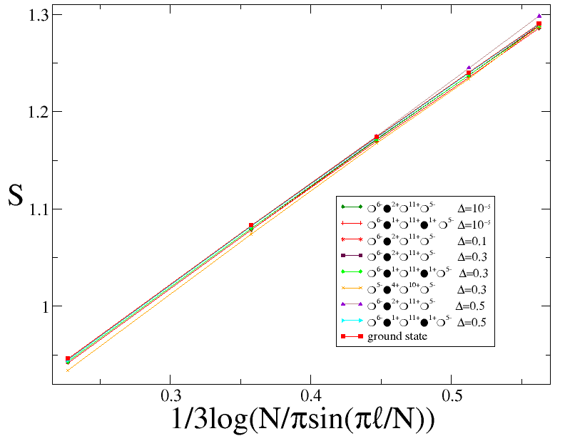
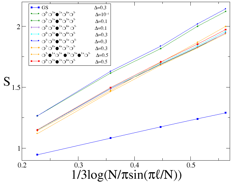
3.5.1 Bethe equations and classification of the states.
The Bethe equations (45) can be re-casted in a form that is useful for numerical solutions and for a complete classification of the states. For practical reasons, we consider only the number of sites to be even. We recall that the Hilbert space separates in sector with defined number of reversed spins (with respect to the reference state cf. Eq. (43)), that gives the total spin of the state in the direction . Taking the logarithm of Eq. (45) and posing , we have
| (110) |
Each set of distinct half-odd integer (integer) for even (odd) numbers (defined mod) specifies a set of rapidities, and therefore an eigenstate. For example, in the ground state these numbers take the values
| (111) |
This ground state can be interpreted as the spinon vacuum. Spinons are the elementary excitations of the model. They have spin and obey semionic exclusion statistics (see e.g. [57] for a simple introduction to these excitations). Excited states have a defined number of up-spinon and down-spinon . The total number of spinons is even when is even, while . (Actually for the interacting model different values of are possible when the state has some higher strings, which are non-dispersive. This discussion is too technical for the goals of this manuscript and we remand the interested reader to Ref. [43]). However, we will see that the spinon content is not the most important quantity for the entanglement entropy of excited states.
Employing the property that the quantum numbers are defined mod, we can choose the allowed ones in the sets
| (112) |
Only a subset of these numbers, bounded by a calculable function of and (see again Ref. [43] for the technical details) provides real solutions for the rapidities , and we limited our attention to these states. Fixed the parity of (i.e. of , since is even), any state is defined by taking numbers among the allowed ones in or . The spinon content of the state then follows (see again [57]). Instead of using this standard notation to indicate the states, following Ref. [58], we adopt a more complicated one that is useful to recover the fermionic description of the XX model when (because we want to compare with the results in the previous section). We denote with the spinons with polarization up (down) and with the empty positions that can be occupied by spinons with up (down) polarization. We indicate with an exponent the number of consecutive symbols, for instance stands for
| (113) |
To each sequence of of these symbols and we can associate a single configuration of . For example, the sequence has two up-spinons and no down ones; it follows that we need quantum numbers; the state is fixed by taking from the set the last numbers (see again Ref. [58] for more details). The advantage of this maybe not really intuitive notation is that the rule to recover the fermionic description is very easy: given the sequence one has to associate a fermion for every or [58].
Once we have the set for each state we are interested in, we use the Newton method to solve the Bethe equations. We limit ourself to the two-spinon and four-spinon sector of the spectrum (but we could easily consider other states). We also select states with real rapidities, to avoid problems with strings contributions, that however can be handled following Ref. [43].
3.5.2 Results.
The main feature we want to check here is if the conformal scaling (2) with an effective central charge is still valid for given excited states when we add the interaction to the XX chain considered in the previous section. The prediction for the XX is based on the discontinuities of (cf. Eq. (21)). In order to predict the result at we exploit the mapping between the fermionic description and the spinonic one at . Once we have the fermionic picture associated to the state, we have for . In order to check if the logarithmic scaling is obeyed, we plot against in Eq. (35), so that if the dependence is linear, the slope gives automatically the central charge of the effective Hamiltonian. In Fig. 8 (left) we display some states in the two-spinon and four-spinon sectors. We choose these states in such a way that in the limit , the corresponding fermionic structure has two discontinuities. For example, the state corresponds to the fermion representation , having two discontinuities in . For , we know from the previous section, that all these states are described by Eq. (2) with effective central charge , as in the ground-state. Fig. 8 (left) provides a clear evidence that the asymptotic behavior of the entropy for does not depend on , at least in the considered range . In the figure we also report the ground-state value for for comparison.
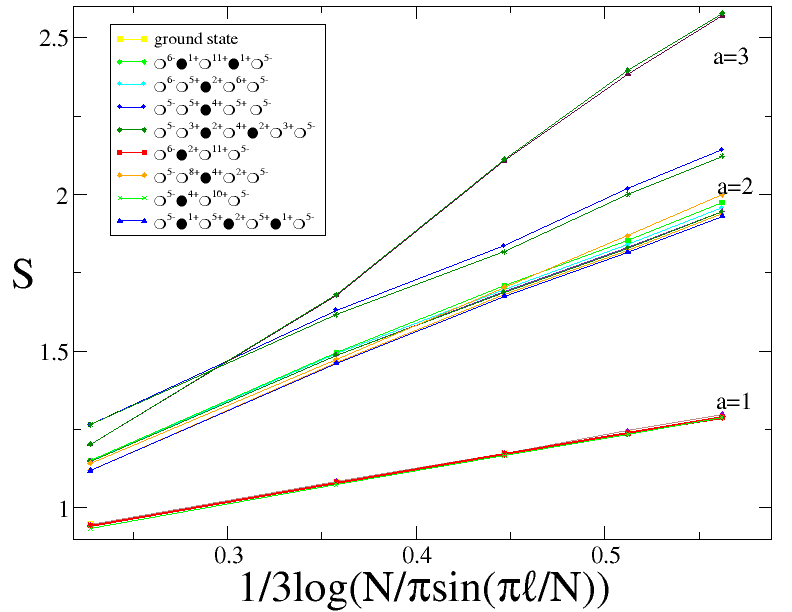
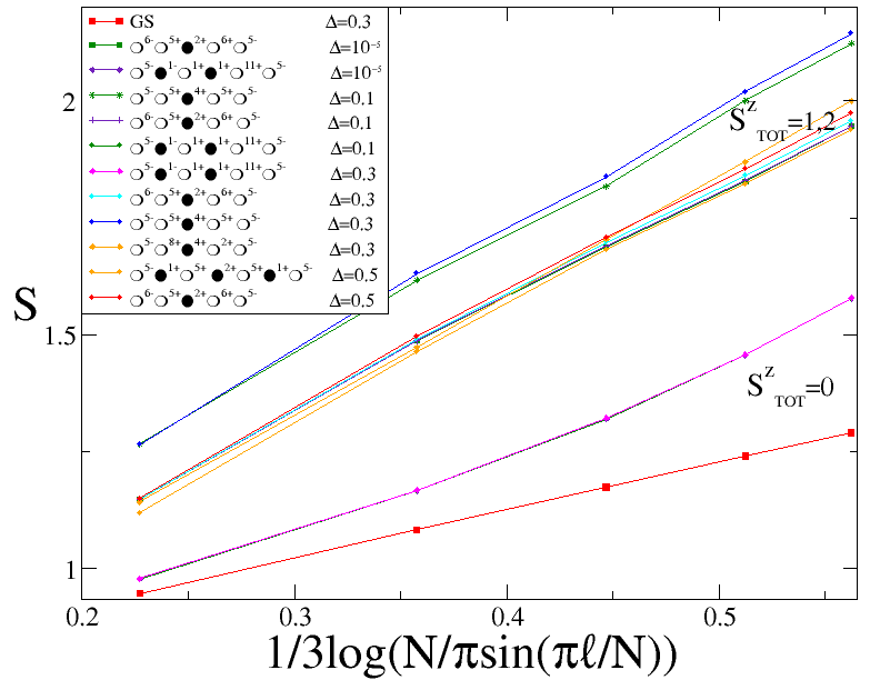
In Fig. 8 (right) we report the entropy for some states whose fermionic description contains four discontinuities. Again we can observe that the data support the logarithmic behavior in Eq. (2). The slope is different from the ground-state one, and indeed a naïve fit (i.e. ignoring further corrections to the scaling that at are important) of the constant gives , which is in agreement with the XX prediction . Moreover, the state shows that the additive constant in Eq. (2) depends dramatically on the details of the state (as we already know in the XX model). In Fig. 9 (right) we show the dependence on the spinon contribution of the additive constant. In Fig. 9 (left) we report the von Neumann entropy for all states and values of we calculated. The changing in behavior for different numbers of discontinuities is clearly visible. In this figure we also report two (almost indistinguishable) states that have six discontinuities in the fermionic description and so are expected to have . There are strong crossover effects preventing us to extract clearly the value of for such small subsystems, but the data are clearly in the right direction. This crossover is expected from the results for the XX model: when having 6 discontinuities in a chain of 24 spins, we expect approximately linear behavior in up to , and in fact in the figure the crossover takes place around . A quantitative understanding of this crossover (even for more excited states) requires larger values of and that are not currently accessible to us.
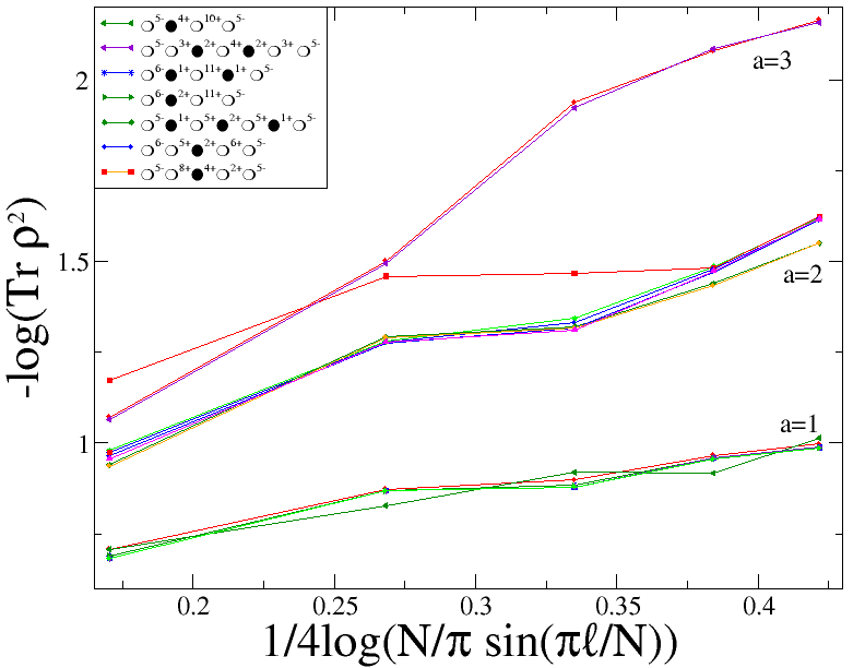
To conclude this section, we also report in Fig. 10 the data for plotted against the logarithm of the conformal distance to check the conformal prediction [4]
| (114) |
for . In fact, if the slope of all the previous curves can be interpreted as the central charge of some effective critical Hamiltonian having this state as a ground-state, not only the entanglement entropy should follow the conformal prediction (2), but also all Rényi entropies should scale according to Eq. (114). And in fact, as for the curves arrange in sectors with approximately similar slopes. Strong even-odd oscillations of the Rényi entropies prevent us from any reliable quantitative analysis, as it is the case in the ground-state [49]. Again it is visible the same structure observed for the von Neumann entropy. However, naïve fits give reasonable estimations of the effective central charges for the two lowest sets, but the oscillations (combined with the crossover previously mentioned) spoil the result for the last set for which is expect.
The knowledge of the full reduced density matrix can be also used to calculate the entanglement spectrum (i.e. the distribution of its eigenvalues). However, because of the relative small values of we can access, this is not enough to check recent conformal predictions for the spectrum [59].
4 Summary and discussions
In this paper we considered the entanglement entropy of excited states in spin chains. We provided a full analytical study of the XY model in a transverse magnetic field. We found that the entanglement properties of the excited states depend strongly on the distribution of excitations above the ground state. To characterize them in the thermodynamic limit, we introduced the regularized characteristic function of excitation . The analytic properties of this function (or slight variation of it for critical systems) completely determine the entanglement in the scaling limit . When in a set of non-vanishing measure, we have that the entanglement entropy is extensive in the subset length (i.e. proportional to ). The analytic expression for such states is given by Eq. (19) as we proved by using the Szëgo lemma for block Toeplitz matrices. Oppositely when almost everywhere (as for the ground state) the entanglement entropy always follows the conformal scaling (2), even for non-critical systems (except in the ground-state when the area law holds). The pre-factor (that we indicate as ) is the central charge of a critical, local, translational invariant Hamiltonian, that we built explicitly. In the case of the XX model we proved this result rigorously via the Fisher-Hartwig conjecture. These logarithmic states have a finite-size scaling that is by construction the conformal one in Eq. (2). Oppositely the extensive states have very peculiar finite size scaling with slopes that changes according to the analytic properties of . We have been able to connect these features to the (non-)locality properties of an effective Hamiltonian that can be made local on a wrapped chain.
We also considered the XXZ spin chain, that is solvable by Bethe Ansatz. We used the algebraic construction to calculate exactly the reduced density matrix for finite chains with . The method we developed is ideal to obtain the entanglement entropy of excited states. In fact, while numerical methods based on MPS like DMRG [56] are very effective for the ground-state, they usually work bad for highly excited ones. Our method instead treats on the same foot any eigenstate, that is specified by the quantum numbers related to the spinonic content of the state. This method has the numerical advantage that its complexity increases only in a polynomial way with (while exact diagonalization is exponential). The drawback is that the complexity increases exponentially with and limited our study to . We do not not know whether this is an intrinsic limit of the method, or if our representation of the reduced density matrix can be still drastically optimized to make the procedure more effective. The trickiest point in our derivation was to obtain the homogenous limit from the results in Ref. [22, 23]. If we would have been able to find a more effective way to perform this limit, the method we propose could have been as effective as DMRG. However, even if we could study only subsystem with , we have been able to conclude that the main results obtained analytically for the XX model (at ) remain valid when interaction is turned on. We showed in fact (making the proper mapping between spinonic and fermionic excitation at ) that all the states that are logarithmic for maintain this property with the same prefactor and with a non-universal additive constant that depends very smoothly on (as for the ground-state [55]).
After this study, the characterization of the asymptotic block entanglement of excited states in these two chains is at an advanced level. Few unsolved problems are still present, especially for the XXZ chain, as e.g. the understanding of the string-states and the quantitative description of the crossover between linear and logarithmic behavior. However, the main question that still remains open is how general are these results. The fact that the division among extensive and logarithmic states is conserved when the interaction is introduced, strongly suggests that this phenomenon should be expected for any local spin-chain, with a prefactor that can be predicted after that the relevant excitations have been identified. In fact, in the interacting system (especially for not small) the excited states are complicated linear combinations of the free-particle ones, several degenerations are also removed by , and it is unlikely that such result is only a coincidence. However, we do not have a general proof for this statement. It might be that for low-lying excited states the generalization of the conformal methods of Refs. [4, 5] can give the logarithmic behavior of these states. Anyway, we have shown here that this property is not limited to low-lying states and so a more general proof would be desirable. Another very interesting question would be to understand how these results are affected by quenched disorder. For the ground-state it is known that only the prefactor of the logarithm is changed [60], but the excitations in these systems are so different that major qualitative changes can take place. Finally, it should be possible to generalize the methods employed for ground-states of free lattice models in higher dimensional systems (as those reviewed in Ref. [2]) to the excited states of the same models. Some results in this direction, relevant for the physics of black holes are reported in Ref. [9].
Acknowledgments
We are extremely grateful to Jean-Sebastian Caux for his interest in this project and for continuous fruitful discussions. We thank G. Sierra and M. Ibanez for sharing with us their unpublished results and for useful discussions. We thank F. Colomo and F. Franchini for discussions. PC benefited of a travel grant from ESF (INSTANS activity).
References
References
- [1] L. Amico, R. Fazio, A. Osterloh, and V. Vedral, Entanglement in Many-Body Systems, Rev. Mod. Phys. 80, 517 (2008) [quant-ph/0703044].
- [2] J. Eisert, M. Cramer, and M. B. Plenio, Area laws for the entanglement entropy - a review, Rev. Mod. Phys. XX, XXX (2009) [0808.3773].
- [3] Entanglement entropy in extended systems, P. Calabrese, J. Cardy, and B. Doyon Eds., J. Phys. A, Special issue, in preparation.
- [4]
P. Calabrese and J. Cardy,
Entanglement entropy and quantum field theory,
J. Stat. Mech. P06002 (2004) [hep-th/0405152];
P. Calabrese and J. Cardy, Entanglement entropy and quantum field theory: a non-technical introduction, Int. J. Quant. Inf. 4, 429 (2006) [quant-ph/0505193]. - [5] P. Calabrese and J. Cardy, Entanglement entropy and conformal field theory, 0905.4013.
- [6] C. Holzhey, F. Larsen, and F. Wilczek, Geometric and Renormalized Entropy in Conformal Field Theory, Nucl. Phys. B 424, 443 (1994) [hep-th/9403108].
- [7]
G. Vidal, J. I. Latorre, E. Rico, and A. Kitaev,
Entanglement in quantum critical phenomena,
Phys. Rev. Lett. 90, 227902 (2003) [quant-ph/0211074]
J. I. Latorre, E. Rico, and G. Vidal, Ground state entanglement in quantum spin chains, Quant. Inf. and Comp. 4, 048 (2004) [quant-ph/0304098]. - [8]
M. Caraglio and F. Gliozzi, Entanglement Entropy and Twist Fields,
JHEP 0811: 076 (2008) [0808.4094];
S. Furukawa, V. Pasquier, and J. Shiraishi, Mutual Information and Compactification Radius in a c=1 Critical Phase in One Dimension, Phys. Rev. Lett. 102, 170602 (2009) [0809.5113];
P. Calabrese, J. Cardy, and E. Tonni, Entanglement entropy of two disjoint intervals in conformal field theory, [0905.2069]. - [9]
S. Das and S. Shankaranarayanan, How robust is the entanglement entropy-area relation?,
Phys. Rev. D 73 (2006) 121701 [gr-qc/0511066];
S. Das and S. Shankaranarayanan, Where are the black hole entropy degrees of freedom ?, Class. Quant. Grav. 24, 5299 (2007) [gr-qc/0703082];
S. Das, S. Shankaranarayanan, and S. Sur, Power-law corrections to entanglement entropy of horizons, Phys. Rev. D 77, 064013 (2008) [0705.2070]. - [10] M. Requardt, Entanglement Entropy for Ground states, Low lying and Highly Excited Eigenstates of General (Lattice) Hamiltonians, hep-th/0605142.
- [11] F. C. Alcaraz and M. S. Sarandy, Finite-size corrections to entanglement in quantum critical systems, Phys. Rev. A 78, 032319 (2008) [0808.0020].
- [12] L. Masanes, An area law for the entropy of low-energy states, 0907.4672.
- [13] J. I. Latorre and A. Riera, A short review on entanglement in quantum spin systems, 0906.1499.
- [14]
I. Peschel, M. Kaulke, and O. Legeza,
Density-matrix spectra for integrable models,
Ann. Physik (Leipzig) 8 (1999) 153 [cond-mat/9810174];
I. Peschel and M.-C. Chung, Density Matrices for a Chain of Oscillators, J. Phys. A 32 8419 (1999) [cond-mat/9906224];
M.-C. Chung and I. Peschel, Density-Matrix Spectra of Solvable Fermionic Systems, Phys. Rev. B 64, 064412 (2001) [cond-mat/0103301];
I. Peschel, Calculation of reduced density matrices from correlation functions, J. Phys. A 36, L205 (2003) [cond-mat/0212631];
I. Peschel, On the reduced density matrix for a chain of free electrons, J. Stat. Mech. (2004) P06004 [cond-mat/0403048]. - [15] I. Peschel, On the entanglement entropy for a XY spin chain, J. Stat. Mech. (2004) P12005 [cond-mat/0410416]
- [16] I. Peschel and V. Eisler, Reduced density matrices and entanglement entropy in free lattice models, 0906.1663.
- [17] B.-Q. Jin, V. E. Korepin, Quantum Spin Chain, Toeplitz Determinants and Fisher-Hartwig Conjecture, J. Stat. Phys. 116, 79 (2004) [quant-ph/0304108].
- [18]
A. R. Its, B.-Q. Jin, and V. E. Korepin,
Entanglement in XY Spin Chain,
J. Phys. A 38, 2975 (2005) [quant-ph/0409027];
F. Franchini, A. R. Its, and V. E. Korepin, Rényi Entropy of the XY Spin Chain, J. Phys. A 41 (2008) 025302 [0707.2534]. - [19] F. Igloi and R. Juhasz, Exact relationship between the entanglement entropies of XY and quantum Ising chains, Europhys. Lett. 81, 57003 (2008) [0709.3927].
- [20] H. Bethe, Zur theorie der metalle, Z. Phys. 71, 205 (1931).
- [21] M. Gaudin, “La fonction d’onde de Bethe”, Masson (Paris) (1983).
- [22] N. Kitanine, J. M. Maillet, and V. Terras, Form factors of the XXZ Heisenberg spin-1/2 finite chain Nucl. Physics B 554 647 (1999) [math-ph/9807020].
- [23] N. Kitanine, J. M. Maillet, and V. Terras, Correlation functions of the XXZ Heisenberg spin-1/2 chain in a magnetic field, Nucl. Phys. B 567, 554 (2000) [math-ph/9907019].
- [24]
M. Rigol, V. Dunjko, and M. Olshanii,
Thermalization and its mechanism for generic isolated quantum systems,
Nature 452, 854 (2008) [0708.1324];
A. Silva, The statistics of the work done on a quantum critical system by quenching a control parameter, Phys. Rev. Lett. 101, 120603 (2008) [0806.4301];
L. Campos Venuti and P. Zanardi, Unitary equilibrations: probability distribution of the Loschmidt echo, [0907.0683];
G. Biroli, C. Kollath, A. Laeuchli; Does thermalization occur in an isolated system after a global quantum quench? [0907.3731];
F. N.C. Paraan and A. Silva, Quantum quenches in the Dicke model: statistics of the work done and of other observables, 0905.4833;
M. Rigol, Quantum quenches and thermalization in one-dimensional fermionic systems, [0908.3188];
M. Fagotti and P. Calabrese, to appear. - [25] P. Calabrese and J. Cardy, Evolution of Entanglement entropy in one dimensional systems, J. Stat. Mech. P04010 (2005) [cond-mat/0503393].
- [26]
G. De Chiara, S. Montangero, P. Calabrese, and R. Fazio
Entanglement Entropy dynamics in Heisenberg chains,
J. Stat. Mech. P03001 (2006) [cond-mat/0512586];
J. Eisert and T. J. Osborne, General Entanglement Scaling Laws from Time Evolution, Phys. Rev. Lett. 97, 150404 (2006) [quant-ph/0603114];
S. Bravyi, M. B. Hastings, and F. Verstraete, Lieb-Robinson Bounds and the Generation of Correlations and Topological Quantum Order, Phys. Rev. Lett. 97, 050401 (2006) [quant-ph/0603121];
A. Laeuchli and C. Kollath, Spreading of correlations and entanglement after a quench in the Bose-Hubbard model, J. Stat. Mech. (2008) P05018 [0803.2947];
V. Eisler and I. Peschel, Entanglement in a periodic quench, Ann. Phys. (Berlin) 17, 410 (2008) [0803.2655];
P. Calabrese, C. Hagendorf, and P. Le Doussal, Time evolution of 1D gapless models from a domain-wall initial state: SLE continued?, J. Stat. Mech. (2008) P07013 [0804.2431];
M. Znidaric, T. Prosen, and I. Pizorn, Complexity of thermal states in quantum spin chains, Phys. Rev. A 78, 022103 (2008) [0805.4149];
S. R. Manmana, S. Wessel, R. M. Noack, and A. Muramatsu, Time evolution of correlations in strongly interacting fermions after a quantum quench, Phys. Rev. B 79, 155104 (2009) [0812.0561];
V. Eisler, F. Igloi, and I. Peschel, Entanglement in spin chains with gradients, J. Stat. Mech. (2009) P02011 [0810.3788]. - [27] M. Fagotti and P. Calabrese, Evolution of entanglement entropy following a quantum quench: Analytic results for the XY chain in a transverse magnetic field, Phys. Rev. A 78, 010306(R) (2008) [0804.3559].
- [28]
V. Eisler and I. Peschel,
Evolution of entanglement after a local quench,
J. Stat. Mech. P06005 (2007) [cond-mat/0703379];
P. Calabrese and J. Cardy, Entanglement and correlation functions following a local quench: a conformal field theory approach, J. Stat. Mech. (2007) P10004 [0708.3750]; V. Eisler, D. Karevski, T. Platini, and I. Peschel, Entanglement evolution after connecting finite to infinite quantum chains, J. Stat. Mech. (2008) P01023 [0711.0289];
A. Perales and G. Vidal, Entanglement growth and simulation efficiency in one-dimensional quantum lattice systems, Phys. Rev A 78, 042337 (2008) [0711.3676];
I. Klich and L. Levitov, Quantum Noise as an Entanglement Meter, Phys. Rev. Lett. 102, 100502 (2009) [0804.1377];
I. Pizorn and T. Prosen, Operator Space Entanglement Entropy in XY Spin Chains, Phys. Rev. B 79, 184416 (2009) [0903.2432];
B. Hsu, E. Grosfeld, and E. Fradkin, Quantum noise and entanglement generated by a local quantum quench, Phys. Rev. B to appear [0908.2622]. - [29]
F. C. Alcaraz, V. Rittenberg, and G. Sierra,
Entanglement in Far From Equilibrium Stationary States,
Phys. Rev. E 80, 030102(R) (2009) [0905.0211];
V. Eisler and Z. Zimboras, Entanglement in the XX spin chain with an energy current, Phys. Rev A 71, 042318 (2005) [quant-ph/0412118]. - [30] M. Ibanez and G. Sierra, private communication.
- [31] H. Au-Yang and B. McCoy, Theory of layered Ising models. II. Spin correlation functions parallel to the layering, 1974 Phys. Rev. B 10 3885.
- [32]
J. P. Keating and F. Mezzadri,
Random Matrix Theory and Entanglement in Quantum Spin Chains,
Commun. Math. Phys. 252 (2004) 543 [quant-ph/0407047];
J. P. Keating and F. Mezzadri, Entanglement in Quantum Spin Chains, Symmetry Classes of Random Matrices, and Conformal Field Theory, Phys. Rev. Lett. 94 (2005) 050501 [quant-ph/0504179]. - [33]
M. E. Fisher and R. E. Hartwig,
Toeplitz determinants: some applications, theorems, and conjectures,
Adv. Chem. Phys. 15, 333 (1968);
P. J. Forrester and N. E. Frankel, Applications and generalizations of Fisher-Hartwig asymptotics, J. Math. Phys. 45, 2003 (2004) [math-ph/0401011];
E. L. Basor and K. E. Morrison, Linear Algebra and Its Applications 202, 129 (1994). - [34]
M. Srednicki, Entropy and Area,
Phys. Rev. Lett. 71 (1993) 666 [hep-th/9303048];
M. M. Wolf, F. Verstraete, M. B. Hastings, and J. I. Cirac, Area laws in quantum systems: mutual information and correlations, Phys. Rev. Lett. 100, 070502 (2008) [0704.3906]. - [35] V. E. Korepin, N. M. Bogoliubov and A. G. Izergin, Quantum Inverse Scattering Method and Correlation Functions, Cambridge University Press (1993).
- [36]
N. Kitanine, J.M. Maillet, N.A. Slavnov, V. Terras,
Spin-spin correlation functions of the XXZ-1/2 Heisenberg chain in a
magnetic field,
Nucl. Phys. B 641 (2002) 487 [hep-th/0201045];
N. Kitanine, J. M. Maillet, N. A. Slavnov, V. Terras, Large distance asymptotic behavior of the emptiness formation probability of the XXZ spin-1/2 Heisenberg chain, J.Phys. A 35 (2002) L753 [hep-th/0210019];
N. Kitanine, J. M. Maillet, N. A. Slavnov, V. Terras, Master equation for spin-spin correlation functions of the XXZ chain, Nucl.Phys. B 712 (2005) 600 [hep-th/0406190];
N. Kitanine, J. M. Maillet, N. A. Slavnov, V. Terras, Dynamical correlation functions of the XXZ spin-1/2 chain, Nucl.Phys. B 729 (2005) 558 [hep-th/0407108];
N. Kitanine, J.M. Maillet, N.A. Slavnov, V. Terras, On the spin-spin correlation functions of the XXZ spin-1/2 infinite chain, J.Phys. A 38 (2005) 7441 [hep-th/0407223]. - [37]
N. Kitanine, K. Kozlowski, J. M. Maillet, G. Niccoli, N. A. Slavnov, V. Terras,
Correlation functions of the open XXZ chain I,
J. Stat. Mech P10009, 2007 [0707.1995];
N. Kitanine, K. Kozlowski, J. M. Maillet, G. Niccoli, N. A. Slavnov, V. Terras, Correlation functions of the open XXZ chain II, J. Stat. Mech. (2008) P07010 [0803.3305]. - [38]
J.-S. Caux and J.-M. Maillet,
Computation of dynamical correlation functions of Heisenberg chains in a field,
Phys. Rev. Lett. 95, 077201 (2005);
J.-S. Caux, R. Hagemans and J.-M. Maillet, Computation of dynamical correlation functions of Heisenberg chains: the gapless anisotropic regime, J. Stat. Mech. P09003 (2005). - [39]
R. G. Pereira, J. Sirker, J.-S. Caux, R. Hagemans, J. M. Maillet,
S. R. White, I. Affleck,
The dynamical spin structure factor for the anisotropic spin-1/2 Heisenberg
chain,
Phys. Rev. Lett. 96, 257202 (2006) [cond-mat/0603681];
R. G. Pereira, J. Sirker, J.-S. Caux, R. Hagemans, J. M. Maillet, S. R. White, I. Affleck, Dynamical structure factor at small q for the XXZ spin-1/2 chain, J. Stat. Mech. (2007) P08022 [0706.4327]. - [40]
J.-S. Caux and P. Calabrese,
Dynamical density-density correlations in the one-dimensional Bose gas,
Phys. Rev. A 74, 031605 (2006);
J.-S. Caux, P. Calabrese and N. A. Slavnov, One-particle dynamical correlations in the one-dimensional Bose gas, J. Stat. Mech. P01008 (2007). - [41] A. Faribault, P. Calabrese, and J.-S. Caux, Exact mesoscopic correlation functions of the pairing model, Phys. Rev. B 77, 064503 (2008).
- [42]
A. Faribault, P. Calabrese, and J.-S. Caux,
Quantum quenches from integrability: the fermionic pairing model,
J. Stat. Mech. (2009) P03018 [0812.1928];
A. Faribault, P. Calabrese, and J.-S. Caux, Bethe Ansatz approach to quench dynamics in the Richardson model, J. Math. Phys. 50, 095212 (2009) [0908.1675]. - [43] J.-S. Caux Correlation functions of integrable models: a description of the ABACUS algorithm, J. Math. Phys. 50, 095214 (2009) [0908.1660].
- [44] J. Sato and M. Shiroishi, Density matrix elements and entanglement entropy for the spin-1/2 XXZ chain at =1/2, J. Phys. A 40, 8739 (2007).
- [45] J. L. Jacobsen and H. Saleur, Exact valence bond entanglement entropy and probability distribution in the XXX spin chain and the Potts model, Phys. Rev. Lett. 100, 087205 (2008).
- [46]
J. Damerau, F. Göhmann, N. P. Hasenclever, and A. Klümper,
Density matrices for finite segments of Heisenberg chains of arbitrary length
J. Phys. A 40, 4439 (2007);
H. E. Boos, J. Damerau, F. Göhmann, A. Klümper, J. Suzuki, and A. Weisse, Short-distance thermal correlations in the XXZ chain, J. Stat. Mech. P08010 (2008);
C. Trippe, F. Göhmann, A. Klümper, Short-distance thermal correlations in the massive XXZ chain, [0908.2232]. - [47] J. Sato, M. Shiroishi, M. Takahashi, Exact evaluation of density matrix elements for the Heisenberg chain , J. Stat. Mech. P12017 (2006).
- [48] A. V. Razumov and Y. G. Stroganov, Spin chains and combinatorics, J. Phys. A 34, 3185 (2001); Y. G. Stroganov, The Importance of being Odd, J. Phys. A 34, L179 (2001).
- [49] B. Nienhuis, M. Campostrini, and P. Calabrese, Entanglement, combinatorics and finite-size effects in spin-chains, J. Stat. Mech. (2009) P02063 [0808.2741].
- [50] L. Banchi, F. Colomo, and P. Verrucchi, When finite-size corrections vanish: The S=1/2 XXZ model and the Razumov-Stroganov state, Phys. Rev. A 80, 022341 (2009) [0906.3703].
- [51] N. A. Slavnov, On scalar products in the algebraic Bethe ansatz, Teor. Mat. Fiz. 79, 232 (1989).
- [52] V. E. Korepin, Calculation of norms of Bethe wave functions, Commun. Math. Phys. 86, 391 (1982).
- [53] A. G. Abanov and V. E. Korepin, On the probability of ferromagnetic strings in antiferromagnetic spin chains, Nucl. Phys. B 647, 565 (2002).
- [54] F. Colomo and A. G. Pronko, Emptiness formation probability in the domain-wall six-vertex model, Nucl. Phys. B 798, 340 (2008) [0712.152].
- [55] P. Calabrese, M. Campostrini, B. Nienhuis et al., in preparation.
- [56]
U. Schollwoeck, The density-matrix renormalization group,
Rev. Mod. Phys. 77, 259 (2005) [cond-mat/0409292];
F. Verstraete, J.I. Cirac, and V. Murg, Matrix Product States, Projected Entangled Pair States, and variational renormalization group methods for quantum spin systems, Adv. Phys. 57, 143 (2008) [0907.2796];
J.I. Cirac and F. Verstraete, Renormalization and tensor networks in spin chains and lattices, J. Phys. A, to appear. - [57] M. Karbach, K. Hu, and G. Muller, Introduction to the Bethe ansatz II, Computers in Physics 12, 565 (1998) [cond-mat/9809163]
- [58] M. Arikawa, M. Karbach, G. Muller, and K. Wiele, Spinon excitations in the XX chain: spectra, transition rates, observability, J. Phys. A 39 (2006 10623 [cond-mat/0605345].
- [59] P. Calabrese and A. Lefevre, Entanglement spectrum in one-dimensional systems, Phys. Rev. A 78, 032329 (2008).
- [60]
G. Refael and J. E. Moore,
Entanglement entropy of random quantum critical points in one dimension,
Phys. Rev. Lett. 93, 260602 (2004) [cond-mat/0406737];
G. Refael and J. E. Moore, Criticality and entanglement in random quantum systems, J. Phys. A, to appear [0908.1986].