Turbo NOC: a framework for the design of Network On Chip based turbo decoder architectures
Abstract
This work proposes a general framework for the design and simulation of network on chip based turbo decoder architectures. Several parameters in the design space are investigated, namely the network topology, the parallelism degree, the rate at which messages are sent by processing nodes over the network and the routing strategy. The main results of this analysis are: i) the most suited topologies to achieve high throughput with a limited complexity overhead are generalized de-Bruijn and generalized Kautz topologies; ii) depending on the throughput requirements different parallelism degrees, message injection rates and routing algorithms can be used to minimize the network area overhead.
I Introduction
In the last years wireless communication systems coped with the problem of delivering reliable information while granting high throughput. This problem has often been faced resorting to channel codes able to correct errors even at low signal to noise ratios. As pointed out in Table I in [1], several standards for wireless communications adopt binary or double binary turbo codes [2, 3] and exploit their excellent error correction capability. However, due to the high computational complexity required to decode turbo codes, optimized architectures (e.g. [4], [5]) have been usually employed. Moreover, several works addressed the parallelization of turbo decoder architectures to achieve higher throughput. In particular, many works concentrate on avoiding, or reducing, the collision phenomenon that arises with parallel architectures (e.g. [6, 7, 8, 9]).
Although throughput and area have been the dominant metrics driving the optimization of turbo decoders, recently, the need for flexible systems able to support different operative modes, or even different standards, has changed the perspective. In particular, the so called software defined radio (SDR) paradigm made flexibility a fundamental property [10] of future receivers, which will be requested to support a wide range of heterogeneous standards. Some recent works (e.g. [1], [11], [12]) deal with the implementation of Application-Specific Instruction-set Processor (ASIP) architectures for turbo decoders. In order to obtain architectures that achieve both high throughput and flexibility multi-ASIP is an effective solution. Thus, together with flexible and high throughput processing elements, a multi-ASIP architecture must feature also a flexible and high throughput interconnection backbone. To that purpose, the Network-On-Chip (NOC) approach has been proposed to interconnect processing elements in turbo decoder architectures designed to support multiple standards [13], [14], [15], [16], [17], [18]. In addition, NOC based turbo decoder architectures have the intrinsic feature of adaptively reducing the communication bandwidth by the inhibition of unnecessary extrinsic information exchange. This can be obtained by exploiting bit-level reliability-based criteria where unnecessary iterations for reliable bits are avoided [19].
In [13], [14], [15] ring, chordal ring and random graph topologies are investigated whereas in [16] previous works are extended to mesh and toroidal topologies. Furthermore, in [17] butterfly and Benes topologies are studied, and in [18] binary de-Bruijn topologies are considered. However, none of these works presents a unified framework to design a NOC based turbo decoder, showing possible complexity/performance trade-offs. This work aims at filling this gap and provides two novel contributions in the area of flexible turbo decoders: i) a comprehensive study of NOC based turbo decoders, conducted by means of a dedicated NOC simulator; ii) a list of obtained results, showing the complexity/performance trade-offs offered by different topologies, routing algorithms, node and ASIP architectures.
The paper is structured as follows: in section II the requirements and characteristics of a parallel turbo decoder architecture are analyzed, whereas in section III NOC based approach is introduced. Section IV summarizes the topologies considered in previous works and introduces generalized de-Bruijn and generalized Kautz topologies as promising solutions for NOC based turbo decoder architectures. In section V three main routing algorithms are introduced, whereas in section VI the Turbo NOC framework is described. Section VII describes the architecture of the different routing algorithms considered in this work, section VIII presents the experimental results and section IX draws some conclusions.
II System requirement analysis
A parallel turbo decoder can be modeled as processing elements that need to read from and write to memories. Each processing element, often referred to as soft-in-soft-out (SISO) module, performs the BCJR algorithm [20], whereas the memories are used for exchanging the extrinsic information among the SISOs. The decoding process is iterative and usually each SISO performs sequentially the BCJR algorithm for the two constituent codes used at the encoder side; for further details on the SISO module the reader can refer to [21]. As a consequence, each iteration is made of two half iterations referred to as interleaving and de-interleaving. During one half iteration the extrinsic information produced by SISO at time () is sent to the memory at the location , where and are functions of and derived from the permutation law ( or interleaver) employed at the encoder side. Thus, the time required to complete the decoding is directly related to the number of clock cycles necessary to complete a half iteration. Without loss of generality, we can express the number of cycles required to complete a half iteration () as
| (1) |
where is the total number of trellis steps in a data frame, is the number of trellis steps processed by each SISO, is the SISO output rate, namely the number of trellis steps processed by a SISO in a clock cycle, and is the interconnection structure latency. Thus, the decoder throughput expressed as the number of decoded bits over the time required to complete the decoding process is
| (2) |
where is the clock frequency, is the number of iterations, for binary codes and for double binary codes. When the interconnection structure latency is negligible with respect to the number of cycles required by the SISO, we obtain
| (3) |
Thus, to achieve a target throughput and satisfactory error rate performance, a proper number of iterations should be used. The minimum () to satisfy with iterations can be estimated from (3) for some ASIP architectures available in the literature. If we consider , as in [1], [12], ranges in [5, 37] to achieve Mb/s (see Table I). It is worth pointing out that the values in Table I represent the average numbers of cycles required by the SISO to update the soft information of one bit (see Table VI in [1] and Table I in [12]). Moreover, strongly depends on the internal architecture of the SISO and in general tends to increase with the code complexity. As a consequence, several conditions can further increase , namely 1) interconnection structures with larger ; 2) higher values; 3) higher ; 4) higher ; 5) lower clock frequency. Thus, we consider as relevant for investigation a slightly wider range for : .
III Network based approach
The NOC approach [23] has been proposed as a general methodology to interconnect heterogeneous intellectual properties (IP) in complex systems on chip (inter-IP interconnection). Recent works deal with methodologies to design application specific NOCs (e.g. [24]) where the NOC is tailored around a particular application or group of applications. In this scenario, turbo decoder architectures are a common IP required in physical layer chips for modern communication standards. In this work, as in some previous papers, e.g. [13], [16], [18] we concentrate on the problem of interconnecting the main building blocks of a parallel turbo decoder, namely we focus on the intra-IP interconnection problem [25], and we do not deal with the general problem of connecting the turbo decoder IP to other receiver modules through an inter-IP interconnection network. To that purpose, it is worth pointing out that statistical characterization of communication patterns, which is one of the most relevant aspects in the design of application specific NOCs, is not required in turbo decoders, as communication patterns depend on . As a consequence, given a set turbo codes with the corresponding laws, the intra-IP communication patterns are deterministic. Thus, the challenge of NOC based turbo decoder architectures is to find one or more sets of parameters that match throughput constraints for all supported standards with a reduced complexity overhead. This set of parameters includes , , the topology and the routing algorithm.
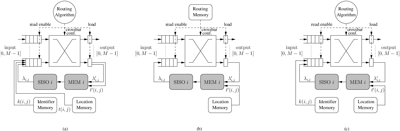
A NOC based turbo decoder architecture relies on nodes connected through a proper topology where the extrinsic information is sent over the network according to a certain routing algorithm. We assume that each node has a certain number of input and output ports (), a FIFO for each input, a crossbar to connect each input FIFO to a proper output and an output register, as shown in Fig. 1. Furthermore, each node has a local SISO (SISO ) that sends extrinsic information over the network through the labeled input port and a local memory (MEM ) that receives extrinsic information from the network through the labeled output port.
Three possible node architectures, shown in Fig. 1, can be conceived to implement the node.
First node architecture
In each half iteration a SISO sends messages where every message is made of a payload containing the extrinsic information and the location of the memory where the extrinsic information will be written (), and a header containing the identifier of the destination node (). As a consequence, the node should contain a memory to store (Identifier Memory), a memory to store (Location Memory) and a routing algorithm to properly route messages through the network (see Fig. 1 (a)).
Second node architecture
Since the permutation law defined by the interleaver is known a-priori, the path followed by a message during an interleaving (or de-interleaving) half iteration can be precalculated and stored as a routing information into a routing memory for each node. This approach reduces the data width of FIFOs, crossbars and registers as neither nor are sent over the network. The location where received messages () will be stored () can be also precalculated and stored into a Location Memory (see Fig. 1 (b)).
Third node architecture
Since the routing memory foot-print can be relevant, a hybrid solution is obtained by precalculating and storing only , whereas the routing is managed by a routing algorithm (see Fig. 1 (c)). This solution does not require a Routing Memory and employs a smaller payload with respect to the solution depicted in Fig. 1 (a). On the other hand, the first approach (Fig. 1 (a)) directly supports adaptive bandwidth reduction techniques, whereas, neither the second nor the third (Fig. 1 (b) and (c)) do.

IV Topologies
As highlighted in [16] and [18] the choice of topologies and routing algorithms impacts both on throughput and complexity. As a consequence, given a certain parallelism degree , topologies with a small node degree () as rings () keep the network complexity overhead limited. On the other hand, topologies with a higher node degree as toroidal meshes () can increase the throughput. Since interleavers tend to spread the extrinsic information almost uniformly among the memories, we consider fixed degree topologies where every node has the same degree . Among fixed degree topologies we included rings and toroidal mesh networks as in [13] and [16]. Moreover, since de-Bruijn topologies have logarithmic diameter, they are good candidates to reduce the latency of the network in turbo decoder architectures, as investigated in [18]. A de-Bruijn topology is made of nodes labeled by an array of elements, each element is taken from an alphabet with symbols. Each node is connected to the nodes whose labels are obtained by left-shifting the node-label array and by placing in the rightmost position a symbol from . As a consequence, each node is connected to nodes () and the number of nodes in the network is . Thus, in general, de-Bruijn topologies for given and values not always exist. This limitation can be overcome by using generalized de-Bruijn topologies [26]. A further limitation of de-Bruijn and generalized de-Bruijn topologies are self loops that are present in some nodes (e.g. the node with label zero).

This limitation is overcome by Kautz topologies where nodes are labeled as in de-Bruijn topologies but avoiding sequences with equal symbols in consecutive positions of the node-label array (Kautz sequences). Then, node connections are obtained as for de-Bruijn topologies, where the symbol placed in the rightmost position of the node-label array is taken from , subject to the constraint that the obtained node-label array is a Kautz sequence. As a consequence, each node is connected to nodes () and the number of nodes in the network is . Thus, as for de-Bruijn topologies, Kautz topologies for assigned and values not always exist. This problem is eliminated by using generalized Kautz topologies [27].
Moreover, we included in our investigation honeycomb networks that, as suggested in [28], are alternatives to toroidal meshes that reduce nodes degree to . Thus, we have that rings, honeycombs and toroidal meshes are represented as undirected graphs, whereas de-Bruijn (generalized de-Bruijn) and Kautz (generalized Kautz) correspond to directed graphs.
V Routing algorithms
Since in turbo decoder architectures the achieved throughput is a key objective, we should try to deliver messages following the shortest available path. Furthermore the NOC must grant that all messages are delivered to the destination, namely dropping of messages to avoid dead-locks is not allowed as it could impair the decoder correction capability. As highlighted in [18] shortest-path based routing algorithms are suited to achieve high throughput and grant message delivery. In the following we will consider both single-shortest-path (SSP) and all-local-shortest-path (ASP) based routing algorithms. In SSP algorithms only one shortest-path from each node to each node is considered, whereas ASP algorithms rely on the fact that in a topology two nodes and may be connected by more shortest-paths. At each node , the actual routing choice toward node must be made by selecting one destination node directly connected to and belonging to a set defined as the set of all nodes adjacent to and placed on a shortest path between and .
Based on shortest-path routing, we tested three strategies to serve the input FIFOs, namely SSP Round-Robin (SSP-RR), SSP FIFO-length (SSP-FL) and ASP FIFO-length with traffic-spreading (ASP-FT). The SSP-RR approach is based on a circular serving policy coupled to the SSP approach. The SSP-FL approach serves the input FIFOs based on the number of elements contained in each input FIFO: the longest FIFO is served first and the shortest one is served last. The ASP-FT approach is based on the input FIFO length serving policy, as for SSP-FL, but it is more complex and can be described as follows. Let’s define as the set of input ports in a node that can receive a message from node at time . At time the number of elements contained in the input FIFO associated to port with is . According to Algorithm 1, the ASP-FT routing algorithm chooses and so that
| (4) |
The couples , that satisfy (4) belong to the set . To choose only one couple in we operate a traffic spreading based selection, namely our objective is to spread the traffic as much as possible over the network. To that purpose we use a set of counters (), where each counter is incremented each time a message is sent from node to node through input port . Then, we select the couple , that is associated to the least used path
| (5) |

It is worth pointing out that, shortest-path based routing algorithms do not prevent output ports contention, that is a situation where two or more inputs need to send data to the same output port. Said the set of inputs in node that at time need to send data to output port , the contention problem can be faced by properly choosing an input allowed to send its data to output port . The remaining inputs belonging to can be managed in different ways. In this work we consider the following two approaches: i) storing into the corresponding input FIFO so that we delay a colliding message, in the following we will refer to this approach as delay-colliding-message (DCM); ii) if possible, sending to another output port , send-colliding-message (SCM). The DCM approach aims at reducing the number of hops to deliver a message to its destination, whereas the SCM approach aims at reducing the maximum depth of the input FIFOs.

VI Turbo NOC simulator
The Turbo NOC simulator [29] is a cycle accurate, SystemC [30] based NOC simulator, specifically tailored for turbo decoder architectures. It estimates the throughput and complexity of a parallel NOC based turbo decoder architecture. It requires as inputs the following elements: the topology description in the form of an adjacence matrix, the permutation law used at the encoder and represented as a sequence of integer values, the routing algorithm (SSP-RR, SSP-FL, ASP-FT), the selected approach to handle contention (DCM/SCM) and the description of the key SISO characteristics. The required parameters to describe the SISO architecture, summarized in Fig. 2 are:
- 1.
the window size () [31],
- 2.
- 3.
the order used to send extrinsic informations on the network, namely forward or backward recursion order,
- 4.
the number of clock cycles between two consecutive outputs within a window (),
- 5.
the number of clock cycles between the last output of a window and the first of the successive window ().
The simulator acts in two phases, a static phase (instantiation and binding) and a dynamic phase (cycle accurate simulation). During the static phase, the topology description defines , and all possible paths from one node to the other. The simulator represents the topology as a graph, calculates all the local shortest paths repeating the Floyd-Warshall algorithm on pruned versions of the graph until no more local paths exist between a source node and its adjacent nodes, and stores each result of the Floyd-Warshall algorithm as an array. Then, if a SSP routing algorithm is employed, only the first shortest path array is employed, otherwise all the shortest paths are considered. Moreover, nodes are instantiated and binded according to the assigned topology and each SISO memory is loaded with messages, based on the assigned permutation. The actual decoding process executed by SISO elements is not included in the tool, which only simulates the exchange of extrinsic informations. However, the SISO architecture parameters are employed to initialize a set of counters that are used to send the extrinsic information over the network with the same timing as in the real SISO architecture. The node is described by means of a hardware-description-language-like (hdl-like) model. When the static phase is completed, the simulation starts resorting to the SystemC kernel simulator and performs a cycle accurate hdl-like simulation. The results provided by the Turbo NOC simulator can be divided in two categories: cycle by cycle results and global results. The cycle by cycle results are: i) for each node, the status of each FIFO, ii) for each node the FIFO read enable and the crossbar configuration signals, iii) for each SISO the sequence. The global results are: i) for each FIFO in each node the maximum FIFO size, ii) for each node the minimum, maximum and average latency (in clock cycles) of each received message and the total number of clock cycles to deliver all the messages.
VII Routing algorithm architecture
In order to keep the NOC complexity as small as possible, SSP-RR and SSP-FL routing algorithms have been implemented with architectures (a) and (c) in Fig. 1, whereas the ASP-FT algorithm has been implemented as a routing memory, as in Fig. 1 (b).
VII-A SSP-RR and SSP-FL architectures
The SSP-RR and SSP-FL architectures, thoroughly shown in Fig. 3 and 4, are made of two main parts. The first part sorts the input FIFOs based on the selected priority method (round-robin or FIFO length) and generates signals, , …, , where is the label of the input that is served first and is the label of the input that is served last. The second part serves the input FIFOs according to the order specified by the , …, sequence and generates the read-enable () signals for the FIFOs, the load enable () signals for the output registers and the configuration commands for the crossbar (), where represents the label of the destination node specified by the first message in FIFO . As shown in Fig. 3 (a), in the SSP-RR architecture a rotate register generates the signals. On the other hand, (see Fig. 3 (b)), in the SSP-FL architecture the signals are obtained with a sorting network. In node the sorting network takes as an input the number of elements contained at time in each input FIFO ( with ) and outputs , …, . Both SSP-RR and SSP-FL architectures have been designed as parametric units to support different values.
The generation of the , and signals is enabled by the signals of the input FIFOs and requires the following units: a look-up-table (LUT), reservation blocks and a priority decoder (Fig. 3 (c)). The LUT contains the shortest-path information.
In the SSP approach for each node the set contains only one node, and contains only one port. There is only an output port on node that connects node with node on a shortest path. Thus, every LUT contains locations and the LUT in node at location contains the label of the output port to connect node to node . As a consequence, each LUT is a table that converts destinations () to the corresponding ports ().
The reservation blocks update an -position binary mask to avoid collisions on output ports, whereas the priority decoder implements the selected priority and FIFO management policies by properly generating the the and signals. Since the and signals must be asserted the clock cycle after the and , they are delayed by means of registers. In particular, the and are obtained by delaying the and of one clock cycle.
VII-A1 Reservation block
Each reservation block (Fig. 4 (a)) receives the signals, according to the … sequence, generates a reservation signal () and specifies the output port to be reserved (). The reservation is obtained by updating the , which contains a ‘1’ in the position of a reserved output port and a ‘0’ in the position of a free output port. Each reservation block generates , that is converted by a one-hot decoder into a mask with a ‘1’ in position . The reservation mask is updated () by comparing this mask with the : if the contains a ‘0’ in position the goes to ‘1’.
VII-A2 Priority decoder
The priority decoder is made of two blocks: the read-enable generation block (Fig. 4 (b)) and the destination-port generation block (Fig. 4 (c)).
read-enable generation block
The read-enable generation block is based on few logic gates that act differently depeding on the approach selected to manage the input FIFOs (SCM/): i) in the DCM approach, when FIFO is not empty (=‘0’) is obtained by combining one-hot representation with the corresponding signal. ii) in the SCM approach, when FIFO is not empty (=‘0’) is based on that is a set of signals produced by the destination-port generation block, where ‘0’ when ‘0’ and , namely the output port with label is used only for messages whose destination is the node itself (Fig. 4 (c)).
destination-port generation block
This is an array of multiplexers, where each multiplexer in position implements when ‘1’. On the other hand, must take the value of an un-reserved output port when ‘0’. This is obtained by means of the permutation network implemented by the multiplexers in position with whose outputs () are
| (6) |
and for
| (7) |
where
| (8) |
and if , then .
VII-B ASP-FT architecture
The ASP-FT algorithm is simply implemented by means of a routing memory. As a consequence, DCM and SCM approaches are integrated by filling the routing memory with the appropriate configuration words. Each word is the concatenation of the , … signals with the , …, signals. In order to reduce the word width, the , …, signals, which can be represented on bits, are coded into a crossbar configuration word (). Since for an -port crossbar the possible configurations are , is represented on bits. The corresponding decoder is hardwired into the crossbar. Thus, as shown in Fig. 5 the main component in the routing memory architecture is a RAM. The RAM address () is generated by an adder and a register. The adder is incremented when at least one input FIFO is not empty (‘0’) and it is initialized to zero when the half iteration starts (). Moreover, the are forced to ‘0’ when FIFOs are empty.
VII-C Architecture implementation
To achieve high throughput the routing algorithm should be able to serve the input FIFOs in one clock cycle. This requirement, which is an intrinsic feature of the routing memory architecture used for the ASP-FT, implies that the architectures for the SSP-RR and SSP-FL routing algorithms are combinational circuits. As it can be inferred from Fig. 3 and 4 the speed of SSP-RR and SSP-FL architectures depends mainly on , in fact, impacts on the size of several parts of the routing algorithm architectures, namely the sorting network, the shortest-path information LUT, the reservation mask, the priority decoder and on the number of reservation blocks. Given the topologies presented in section IV, we described the SSP-RR and SSP-FL architectures as parametric blocks and we performed the logical synthesis on a 130 nm standard cell technology for . Post synthesis results confirm that a clock frequency of more than 200 MHz is achieved with a complexity that ranges from about 1000 m2 to about 6000 m2.
| =2, ring | =2, generalized Kautz | ||||||||
| =8 | =16 | =32 | =64 | =8 | =16 | =32 | =64 | ||
| =1.00 | SSP-RR (c) | 115.50/1.64 | 132.30/3.85 | 147.06/5.71 | 152.28/6.91 | 104.35/2.05 | 140.85/3.48 | 195.44/5.17 | 270.27/7.17 |
| SSP-FL (c) | 112.89/1.56 | 134.38/3.18 | 147.78/4.41 | 139.86/5.43 | 108.99/1.85 | 149.07/3.21 | 209.06/4.65 | 287.77/6.35 | |
| ASP-FT (b) | 130.15/1.40 | 144.75/2.87 | 152.87/3.97 | 142.35/5.02 | 108.99/1.73 | 149.07/2.90 | 209.06/4.07 | 287.77/5.41 | |
| =0.50 | SSP-RR (c) | 86.15/0.43 | 122.32/1.61 | 133.48/3.96 | 137.77/5.45 | 86.21/0.44 | 131.15/1.33 | 172.91/3.19 | 229.89/5.29 |
| SSP-FL (c) | 86.15/0.42 | 123.71/1.37 | 132.89/3.67 | 130.15/5.17 | 86.15/0.41 | 138.25/1.06 | 188.68/2.62 | 241.94/4.59 | |
| ASP-FT (b) | 86.02/0.49 | 134.53/1.29 | 137.30/3.35 | 130.72/4.80 | 86.15/0.46 | 138.25/1.05 | 188.68/2.38 | 241.94/3.99 | |
| =0.33 | SSP-RR (c) | 57.80/0.41 | 101.10/0.74 | 122.08/2.96 | 125.92/5.01 | 57.86/0.39 | 102.48/0.75 | 155.44/1.82 | 195.76/3.97 |
| SSP-FL (c) | 57.78/0.39 | 100.84/0.72 | 121.58/2.67 | 120.97/4.87 | 57.80/0.38 | 102.21/0.67 | 161.51/1.43 | 207.25/3.28 | |
| ASP-FT (b) | 57.83/0.46 | 100.84/0.81 | 122.70/2.52 | 121.70/4.56 | 57.80/0.44 | 102.21/0.74 | 161.51/1.40 | 207.25/2.94 | |
| =3, honeycomb | =3, generalized Kautz | ||||||||
| =8 | =16 | =32 | =64 | =8 | =16 | =32 | =64 | ||
| =1.00 | SSP-RR (c) | 113.21/1.69 | 184.05/2.29 | 181.27/5.16 | 323.45/6.47 | 156.45/0.83 | 203.74/2.06 | 314.96/3.60 | 428.57/5.84 |
| SSP-FL (c) | 114.83/1.67 | 187.79/2.22 | 179.64/4.37 | 314.96/5.99 | 166.67/0.67 | 229.89/1.93 | 332.41/3.41 | 451.13/5.49 | |
| ASP-FT (b) | 127.93/1.51 | 247.42/1.64 | 242.91/3.62 | 385.85/4.93 | 166.67/0.67 | 250.52/1.58 | 339.94/2.98 | 456.27/4.64 | |
| =0.50 | SSP-RR (c) | 85.96/0.45 | 151.32/0.91 | 160.64/3.52 | 267.26/4.69 | 86.52/0.45 | 152.67/0.86 | 242.91/1.81 | 331.49/3.76 |
| SSP-FL (c) | 85.90/0.43 | 151.52/0.84 | 163.71/3.10 | 261.44/4.20 | 86.52/0.44 | 152.48/0.82 | 241.94/1.66 | 338.03/3.37 | |
| ASP-FT (b) | 85.90/0.49 | 151.32/0.90 | 213.52/2.08 | 305.34/3.48 | 86.52/0.53 | 152.28/0.88 | 244.40/1.58 | 337.08/2.98 | |
| =0.33 | SSP-RR (c) | 57.72/0.40 | 102.48/0.80 | 144.75/2.27 | 223.88/3.49 | 58.00/0.44 | 103.18/0.78 | 167.13/1.56 | 243.90/3.15 |
| SSP-FL (c) | 57.72/0.40 | 102.48/0.79 | 148.88/2.01 | 226.42/3.21 | 58.00/0.44 | 103.09/0.78 | 168.07/1.50 | 240.48/2.96 | |
| ASP-FT (b) | 57.75/0.46 | 102.65/0.86 | 162.38/1.58 | 233.92/2.87 | 58.00/0.50 | 103.09/0.83 | 168.07/1.48 | 242.91/2.70 | |
| =4, toroidal mesh | =4, generalized Kautz | ||||||||
| =8 | =16 | =32 | =64 | =8 | =16 | =32 | =64 | ||
| =1.00 | SSP-RR (c) | 123.84/1.17 | 171.67/2.10 | 187.21/4.24 | 310.08/6.24 | 140.19/0.94 | 268.46/1.56 | 334.26/3.31 | 517.24/5.29 |
| SSP-FL (c) | 129.87/1.14 | 167.83/2.00 | 200.33/3.67 | 323.45/5.77 | 155.24/0.82 | 281.69/1.30 | 347.83/3.13 | 550.46/4.92 | |
| ASP-FT (b) | 165.29/0.69 | 282.35/1.30 | 357.14/2.79 | 497.93/4.52 | 167.13/0.67 | 281.69/1.24 | 397.35/2.49 | 550.46/4.28 | |
| =0.50 | SSP-RR (c) | 86.15/0.46 | 147.78/1.03 | 165.29/2.75 | 260.30/4.58 | 86.52/0.47 | 153.65/0.89 | 248.45/1.91 | 359.28/3.64 |
| SSP-FL (c) | 86.08/0.45 | 151.52/0.95 | 178.31/2.51 | 270.27/4.25 | 86.52/0.46 | 153.85/0.88 | 247.93/1.81 | 360.36/3.50 | |
| ASP-FT (b) | 86.21/0.54 | 152.28/1.05 | 242.42/1.85 | 334.26/3.46 | 86.52/0.57 | 153.85/0.96 | 248.96/1.77 | 360.36/3.27 | |
| =0.33 | SSP-RR (c) | 57.80/0.44 | 102.92/0.93 | 154.64/1.97 | 223.46/3.81 | 58.00/0.46 | 103.54/0.88 | 169.01/1.75 | 248.96/3.46 |
| SSP-FL (c) | 57.80/0.44 | 102.92/0.91 | 163.49/1.79 | 226.42/3.57 | 58.00/0.45 | 103.54/0.86 | 169.25/1.69 | 248.45/3.34 | |
| ASP-FT (b) | 57.83/0.50 | 102.92/0.98 | 166.90/1.79 | 238.57/3.25 | 58.00/0.53 | 103.54/0.92 | 169.25/1.68 | 248.45/3.15 | |
| =2, ring | =2, generalized Kautz | ||||||||
| =8 | =16 | =32 | =64 | =8 | =16 | =32 | =64 | ||
| =1.00 | SSP-RR (c) | 62.56/6.58 | 72.23/15.73 | 81.22/24.45 | 87.04/30.37 | 56.62/8.43 | 77.26/14.10 | 116.01/20.56 | 169.96/26.72 |
| SSP-FL (c) | 62.57/6.84 | 73.89/13.90 | 82.98/18.67 | 88.25/22.11 | 59.52/8.09 | 83.52/13.50 | 125.31/18.55 | 183.79/23.53 | |
| ASP-FT (b) | 71.48/5.93 | 81.57/11.29 | 88.17/15.12 | 91.14/19.36 | 59.52/6.94 | 83.52/10.74 | 125.31/13.90 | 183.79/16.74 | |
| =0.50 | SSP-RR (c) | 49.12/1.80 | 72.36/6.00 | 80.26/15.71 | 86.11/21.02 | 49.13/1.79 | 77.37/4.10 | 114.99/10.17 | 165.12/16.37 |
| SSP-FL (c) | 49.12/1.78 | 73.42/5.10 | 82.28/14.68 | 87.29/20.48 | 49.13/1.78 | 86.74/2.98 | 129.59/8.00 | 186.75/13.78 | |
| ASP-FT (b) | 49.12/2.50 | 82.40/4.93 | 87.48/12.55 | 90.23/18.42 | 49.13/2.39 | 86.74/3.43 | 129.59/7.03 | 186.75/10.80 | |
| =0.33 | SSP-RR (c) | 32.78/1.76 | 63.67/2.09 | 79.52/11.40 | 85.06/19.10 | 32.78/1.76 | 63.83/2.06 | 111.61/4.13 | 162.20/9.53 |
| SSP-FL (c) | 32.78/1.76 | 63.68/2.04 | 81.51/9.65 | 86.27/18.43 | 32.77/1.75 | 63.81/2.01 | 123.57/2.66 | 186.58/6.51 | |
| ASP-FT (b) | 32.78/2.51 | 63.67/3.37 | 86.71/9.32 | 88.90/17.17 | 32.77/2.44 | 63.81/2.99 | 123.57/3.71 | 186.58/6.45 | |
| =3, honeycomb | =3, generalized Kautz | ||||||||
| =8 | =16 | =32 | =64 | =8 | =16 | =32 | =64 | ||
| =1.00 | SSP-RR (c) | 63.28/6.51 | 107.23/8.07 | 103.96/20.19 | 219.19/21.14 | 87.61/2.86 | 118.27/6.64 | 210.05/10.39 | 332.65/16.23 |
| SSP-FL (c) | 64.03/6.67 | 109.73/8.31 | 106.61/16.64 | 214.53/20.29 | 97.37/2.06 | 135.54/6.08 | 220.22/10.86 | 350.29/16.37 | |
| ASP-FT (b) | 72.48/5.74 | 152.42/5.28 | 160.67/11.92 | 313.79/13.45 | 97.37/2.29 | 153.26/4.55 | 239.53/8.07 | 375.55/11.66 | |
| =0.50 | SSP-RR (c) | 49.12/1.80 | 95.52/2.19 | 102.95/12.05 | 213.78/10.75 | 49.16/1.81 | 95.63/2.15 | 185.62/2.91 | 322.18/5.24 |
| SSP-FL (c) | 49.12/1.79 | 95.48/2.13 | 106.06/10.62 | 208.55/9.56 | 49.16/1.81 | 95.69/2.10 | 185.68/2.76 | 346.34/4.32 | |
| ASP-FT (b) | 49.12/2.50 | 95.60/3.05 | 163.71/4.91 | 312.99/6.14 | 49.16/2.63 | 95.69/3.02 | 185.62/3.54 | 348.10/4.60 | |
| =0.33 | SSP-RR (c) | 32.78/1.77 | 63.84/2.08 | 102.14/5.83 | 205.69/5.13 | 32.79/1.79 | 63.89/2.08 | 124.30/2.68 | 235.31/3.96 |
| SSP-FL (c) | 32.78/1.76 | 63.84/2.06 | 108.17/4.43 | 216.03/4.54 | 32.79/1.79 | 63.89/2.07 | 124.27/2.62 | 235.58/3.78 | |
| ASP-FT (b) | 32.78/2.50 | 63.85/2.99 | 123.62/4.18 | 233.35/5.14 | 32.79/2.47 | 63.89/2.95 | 124.30/3.62 | 235.58/4.68 | |
| =4, toroidal mesh | =4, generalized Kautz | ||||||||
| =8 | =16 | =32 | =64 | =8 | =16 | =32 | =64 | ||
| =1.00 | SSP-RR (c) | 70.18/4.23 | 97.20/6.89 | 110.05/13.77 | 202.77/16.59 | 77.99/3.34 | 174.15/3.71 | 215.50/8.33 | 493.89/10.22 |
| SSP-FL (c) | 73.67/4.04 | 96.02/6.58 | 117.84/11.43 | 214.68/15.00 | 86.09/3.21 | 184.17/2.97 | 232.38/8.38 | 516.74/9.82 | |
| ASP-FT (b) | 96.57/2.36 | 184.12/3.13 | 275.76/6.43 | 471.89/9.19 | 97.11/2.35 | 184.17/3.06 | 298.83/5.09 | 516.74/7.61 | |
| =0.50 | SSP-RR (c) | 49.14/1.82 | 95.26/2.32 | 109.34/7.13 | 198.32/7.77 | 49.16/1.82 | 95.75/2.19 | 185.62/2.95 | 350.48/4.47 |
| SSP-FL (c) | 49.14/1.80 | 95.48/2.22 | 119.74/6.10 | 213.85/7.03 | 49.16/1.82 | 95.75/2.17 | 185.96/2.89 | 350.89/4.28 | |
| ASP-FT (b) | 49.14/2.66 | 95.61/3.34 | 185.17/4.03 | 347.12/5.17 | 49.16/2.72 | 95.75/3.15 | 185.90/3.83 | 350.89/4.96 | |
| =0.33 | SSP-RR (c) | 32.78/1.79 | 63.85/2.17 | 110.01/3.59 | 196.55/5.02 | 32.79/1.81 | 63.91/2.15 | 124.37/2.82 | 236.04/4.17 |
| SSP-FL (c) | 32.78/1.78 | 63.85/2.15 | 123.10/2.97 | 216.80/4.56 | 32.79/1.80 | 63.92/2.14 | 124.40/2.78 | 235.94/4.06 | |
| ASP-FT (b) | 32.78/2.42 | 63.85/3.03 | 124.00/3.95 | 234.15/5.26 | 32.79/2.51 | 63.92/3.02 | 124.40/3.72 | 235.94/4.96 | |
VIII Simulations and results
The Turbo NOC simulator has been used to simulate both interleaving and de-interleaving with four significant permutation laws, namely:
- 1.
WiMax interleaver with =2400 and =38
- 2.
UMTS interleaver with =5114 and =40
- 3.
A prunable S-random interleaver [35] with =16384 and =37
- 4.
A circular shifting interleaver [36] with =24576 and =39
We tested the following topologies:
- 1.
ring (R)
- 2.
toroidal mesh (T)
- 3.
honeycomb (H)
- 4.
generalized de-Bruijn (B)
- 5.
generalized Kautz (K)
for , with SSP-RR, SSP-FL and ASP-FT routing algorithms and including DCM and SCM approaches for FIFO management. The SISO architecture parameters were set as follows: , and backward recursion sending order. For each case, the Turbo NOC simulator provided the total number of cycles required to perform a complete iteration (interleaving and de-interleaving), the depth of each FIFO in the network, the content of each routing memory (see Fig. 1 (b)) and the sequence to be stored into the location memory (see Fig. 1 (b) and (c)). As a consequence, for each case we can estimate the achieved throughput for a certain clock frequency with a given number of iterations. Moreover, to characterize the complexity of each solution we give the synthesis results of all simulated networks for a 130 nm standard cell technology. Memories have been generated by means of a 130 nm memory generator. The area results concern all the nodes in the network where each node includes the blocks depicted in Fig. 1 except the SISO and the memory used to store the extrinsic information (shaded gray blocks in Fig. 1). As a significant case of study we consider each extrinsic information value represented on 8 bits. Thus, we represented on 8 bits for all the simulations, except the ones related to the WiMax permutation law. In fact, since the WiMax turbo code is double binary, its extrinsic information is an array made of three log-likelihood ratios, as a consequence a message is represented on 24 bits. Moreover, we consider MHz and ; thus, from (3) we can infer that to sustain a target throughput of Mb/s, we need at least , namely at least for binary codes and at least for double binary codes. However, due to the term in (2), higher values of the product are also of interest.
The analysis of the experimental results obtained with the Turbo NOC simulator shows some interesting general properties.
- 1.
SSP solutions adopting the node architecture depicted in Fig. 1 (a) are the most demanding implementations in terms of area. Since the node architecture in Fig. 1 (c) achieves the same throughput as the solution in Fig. 1 (a) with a lower area, in the following only the node architecture in Fig. 1 (c) will be addressed.
- 2.
The DCM FIFO management method performs better than the SCM one both in terms of throughput and complexity. As a consequence, in the following only results that are referred to the DCM approach will be presented.
- 3.
Generalized de-Bruijn and generalized Kautz topologies achieve nearly the same results both in terms of throughput and complexity. In the following only results obtained with generalized Kautz topologies will be presented.
- 4.
Results tend to be clustered into two families, namely short interleavers (WiMax interleaver with =2400 and UMTS interleaver with =5114) and long interleavers (prunable S-random interleaver with =16384 and circular shifting interleaver with =24576). For the sake of clarity, in the following, only results obtained for the WiMax interleaver (=2400) and circular shifting interleaver (=24576) will be presented.
The most significant experimental results are summarized in Table II and III that refer to the WiMax interleaver with and to the circular shifting interleaver with respectively. Each cell of the two tables gives the throughput in Mb/s and the area in mm2 obtained for different and values, routing algorithms and architectures for the DCM approach. In Table III light-gray, mid-gray and dark-gray cells indicate the highest throughput, the highest area and the lowest area points for each value respectively.
(a) WiMax,

(b) circular shifting interleaver,

(a) WiMax, , ,

(b) WiMax, , ,

(c) circular shifting interleaver, , ,

(d) circular shifting interleaver, , ,

[t]
| top. | routing alg. | Tot. FIFOs | Tot. CB | Tot. reg. | RA/M | IM+LM | Tot. | |||
|---|---|---|---|---|---|---|---|---|---|---|
| area [mm2] | area [mm2] | area [mm2] | area [mm2] | area [mm2] | area [mm2] | |||||
| 2 | R | 64 | 1 | ASP-FT (b) | 11.45 (59.15%) | 0.03 (0.15%) | 0.08 (0.41%) | 6.35 (32.80%) | 1.45 (7.49%) | 19.36 (100%) |
| 2 | R | 64 | 1 | SSP-RR (c) | 27.46 (90.43%) | 0.05 (0.16%) | 0.14 (0.46%) | 0.11 (0.36%) | 2.61 (8.59%) | 30.37 (100%) |
| 2 | R | 8 | 0.33 | SSP-FL/RR (c) | 0.05 (2.84%) | 0.01 (0.57%) | 0.01 (0.57%) | 0.01 (0.57%) | 1.68 (95.45%) | 1.76 (100%) |
| 2 | K | 64 | 0.5 | ASP-FT (b) | 6.53 (60.46%) | 0.03 (0.28%) | 0.08 (0.74%) | 2.71 (25.09%) | 1.45 (13.43%) | 10.80 (100%) |
| 2 | K | 64 | 1 | SSP-RR (c) | 23.81 (89.11%) | 0.05 (0.19%) | 0.14 (0.52%) | 0.11 (0.41%) | 2.61 (9.77%) | 26.72 (100%) |
| 2 | K | 8 | 0.33 | SSP-FL (c) | 0.05 (2.86%) | 0 (0%)(1) | 0.01 (0.57%) | 0.01 (0.57%) | 1.68 (96.00%) | 1.75 (100%) |
| 3 | H | 64 | 1 | ASP-FT (b) | 9.25 (68.77%) | 0.09 (0.67%) | 0.11 (0.82%) | 2.55 (18.96%) | 1.45 (10.78%) | 13.45 (100%) |
| 3 | H | 64 | 1 | SSP-RR (c) | 18.02 (85.24%) | 0.10 (0.47%) | 0.18 (0.85%) | 0.23 (1.09%) | 2.61 (12.35%) | 21.14 (100%) |
| 3 | H | 8 | 0.33 | SSP-FL (c) | 0.05 (2.84%) | 0.01 (0.57%) | 0.01 (0.57%) | 0.01 (0.57%) | 1.68 (95.45%) | 1.76 (100%) |
| 3 | K | 64 | 1 | ASP-FT (b) | 7.86 (67.41%) | 0.09 (0.77%) | 0.11 (0.94%) | 2.15 (18.44%) | 1.45 (12.44%) | 11.66 (100%) |
| 3 | K | 64 | 1 | SSP-FL (c) | 13.15 (80.33%) | 0.10 (0.61%) | 0.18 (1.10%) | 0.33 (2.02%) | 2.61 (15.94%) | 16.37 (100%) |
| 3 | K | 8 | 0.33 | SSP-FL (c) | 0.06 (3.35%) | 0.01 (0.56%) | 0.02 (1.12%) | 0.02 (1.12%) | 1.68 (93.85%) | 1.79 (100%) |
| 4 | T | 64 | 1 | ASP-FT (b) | 5.14 (55.94%) | 0.23 (2.5%) | 0.13 (1.41%) | 2.24 (24.37%) | 1.45 (15.78%) | 9.19 (100%) |
| 4 | T | 64 | 1 | SSP-RR (c) | 13.21 (79.63%) | 0.17 (1.02%) | 0.23 (1.39%) | 0.37 (2.23%) | 2.61 (15.73%) | 16.59 (100%) |
| 4 | T | 8 | 0.33 | SSP-FL (c) | 0.06 (3.35%) | 0.01 (0.56%) | 0.02 (1.12%) | 0.02 (1.12%) | 1.67 (93.85%) | 1.78 (100%) |
| 4 | K | 64 | 1 | ASP-FT (b) | 3.78 (49.67%) | 0.22 (2.89%) | 0.13 (1.71%) | 2.03 (26.68%) | 1.45 (19.05%) | 7.61 (100%) |
| 4 | K | 64 | 1 | SSP-RR (c) | 6.86 (67.12%) | 0.16 (1.57%) | 0.23 (2.25%) | 0.36 (3.52%) | 2.61 (25.54%) | 10.22 (100%) |
| 4 | K | 8 | 0.33 | SSP-FL (c) | 0.06 (3.33%) | 0.10 (0.56%) | 0.02 (1.11%) | 0.03 (1.67%) | 1.68 (93.33%) | 1.80 (100%) |
- (1)
The area and the percentage are not really zero, but they are negligible compared with the IM and LM contribution to the total area.
The most important conclusions that can be derived from results in Table II and III are:
- 1.
The ASP-FT routing algorithm is the best performing solution both in terms of throughput and area when .
- 2.
The routing memory overhead of the ASP-FT algorithm (see Fig. 1 (b)) becomes relevant as decreases and SSP solutions become the best solutions mainly for and .
- 3.
In most cases topologies with =4 achieve higher throughput with lower complexity overhead than topologies with =2 when .
- 4.
In most cases, generalized de-Bruijn and generalized Kautz topologies are the best performing topologies.
As a significant example, in Fig. 6, we show the experimental results obtained with and ASP-FT routing algorithm for the WiMax interleaver with (a) and the circular shifting interleaver with (b). Each point represents the throughtput and the area obtained for a certain topology with a certain parallelism degree . Results referred to the same value are bounded into the same box and a label is assigned to each point to highlight the corresponding topology, namely topologies are identified as R-ring, H-honeycomb, T-toroidal mesh, K-generalized Kautz with the corresponding value (K2, K3, K4).
As it can be observed, generalized Kautz topologies with (K4) are always the best solutions to achieve high throughput with minimum area overhead.
In Fig. 7 significant results extracted from Table II and III are shown in graphical form. In particular, for the ASP-FT routing algorithm is the best solution, whereas for SSP routing algorithms, implemented as in Fig. 1 (c), tend to achieve the same performance as the ASP-FT routing algorithm with lower complexity overhead (see Fig. 7 (a) and (b) for the WiMax interleaver, and Fig. 7 (c) and (d) for the circular shifting interleaver, ).
An interesting phenomenon that arises increasing the interleaver size is the performance saturation that can be observed in the Table III for topologies, namely the throughput tends to saturate and increasing has the effect of augmenting the area with a negligible increase or even with a decrease of throughput. As an example, the generalized Kautz topology with and ASP-FT routing algorithm achieves more than 180 Mb/s with , , . However, the solution with the smallest area is the one obtained with .
The throughput flattening of low topologies can be explained by observing that high values of tend to saturate the network. Furthermore, high values of lengthen the input FIFOs as highlighted in Table IV, where the total area of the network is given as the breakdown of the building blocks, namely the input FIFOs, the crossbars (CB), the output registers, the routing algorithm/memory (RA/M), the identifier memory (IM) and the location memory (LM) is given for some significant cases: the highest throughput (light-gray), the highest area (mid-gray), and lowest area (dark-gray) points for each value in Table III.
IX Conclusions
In this work a general framework to design network on chip based turbo decoder architectures has been presented. The proposed framework can be adapted to explore different topologies, degrees of parallelism, message injection rates and routing algorithms. Experimental results show that generalized de-Bruijn and generalized Kautz topologies achieve high throughput with a limited complexity overhead. Moreover, depending on the target throughput requirements different parallelism degrees, message injection rates and routing algorithms can be used to minimize the network area overhead.
References
- [1] T. Vogt and N. Wehn, “Reconfigurable ASIP for convolutional and turbo decoding in an SDR environment,” IEEE Transactions on VLSI, vol. 16, no. 10, pp. 1309–1320, Oct 2008.
- [2] C. Berrou, A. Glavieux, and P. Thitimajshima, “Near Shannon limit error correcting coding and decoding: Turbo codes,” in IEEE International Conference on Communications, 1993, pp. 1064–1070.
- [3] C. Berrou, M. Jezequel, C. Douillard, and S. Kerouedan, “The advantages of non-binary turbo codes,” in IEEE Information Theory Workshop, 2001, pp. 61–63.
- [4] R. Dobkin, M. Peleg, and R. Ginosar, “Parallel interleaver design and VLSI architecture for low-latency MAP turbo decoders,” IEEE Transactions on VLSI, vol. 13, no. 4, pp. 427–438, Apr 2005.
- [5] M. Martina, M. Nicola, and G. Masera, “A flexible UMTS-WiMax turbo decoder architecture,” IEEE Transactions on Circuits and Systems II, vol. 55, no. 4, pp. 369–373, Apr 2008.
- [6] A. Giulietti, L. V. der Perre, and M. Strum, “Parallel turbo coding interleavers: avoiding collisions in accesses to storage elements,” IET Electronics Letters, vol. 38, no. 5, pp. 232–234, Feb 2002.
- [7] J. Kwak and K. Lee, “Design of dividable interleaver for parallel decoding in turbo codes,” IET Electronics Letters, vol. 38, no. 22, pp. 1362–1364, Oct 2002.
- [8] M. J. Thul, N. Wehn, and L. P. Rao, “Enabling high-speed turbo-decoding through concurrent interleaving,” in IEEE International Symposium on Circuits and Systems, 2002, pp. 897–900.
- [9] A. Tarable and S. Benedetto, “Mapping interleaving laws to parallel turbo decoder architectures,” IEEE Communications Letters, vol. 8, no. 3, pp. 162–164, Mar 2004.
- [10] A. Polydoros, “Algorithmic aspects of radio flexibility,” in IEEE International Symposium on Personal, Indoor and Mobile Communications, 2008, pp. 1–5.
- [11] B. Bougard, R. Priewasser, L. V. der Perre, and M. Huemer, “Algorithm-architecture co-design of a multi-standard FEC decoder ASIP,” in ICT Mobile Summit Conference, 2008.
- [12] O. Muller, A. Baghdadi, and M. Jezequel, “From parallelism levels to a multi-ASIP architecture for turbo decoding,” IEEE Transactions on VLSI, vol. 17, no. 1, pp. 92–102, Jan 2009.
- [13] M. J. Thul, F. Gilbert, and N. Wehn, “Optimized concurrent interleaving architecture for high-throughput turbodecoding,” in IEEE International Conference on Electronics, Circuits and Systems, 2002, pp. 1099–1102.
- [14] ——, “Concurrent interleaving architectures for high-throughput channel coding,” in IEEE International Conference on Acoustics, Speech and Signal Processing, 2003, pp. 613–616.
- [15] F. Speziali and J. Zory, “Scalable and area efficient concurrent interleaver for high throughput turbo-decoders,” in IEEE Euromicro Symposium on Digital System Design, 2004, pp. 334–341.
- [16] C. Neeb, M. J. Thul, and N. Wehn, “Network-on-chip-centric approach to interleaving in high throughput channel decoders,” in IEEE International Symposium on Circuits and Systems, 2005, pp. 1766–1769.
- [17] H. Moussa, O. Muller, A. Baghdadi, and M. .Jezequel, “Butterfly and Benes-based on-chip communication networks for multiprocessor turbo decoding,” in Design, Automation and Test in Europe Conference and Exhibition, 2007, pp. 654–659.
- [18] H. Moussa, A. Baghdadi, and M. .Jezequel, “Binary de Bruijn interconnection network for a flexible LDPC/turbo decoder,” in IEEE International Symposium on Circuits and Systems, 2008, pp. 97–100.
- [19] O. Muller, A. Baghdadi, and M. Jezequel, “Bandwidth reduction of extrinsic information exchange in turbo decoding,” IET Electronics Letters, vol. 42, no. 19, pp. 1104–1105, Sep 2006.
- [20] L. Bahl, J. Cocke, F. Jelinek, and J. Raviv, “Optimal decoding of linear codes for minimizing symbol error rate,” IEEE Transactions on Information Theory, vol. 20, no. 3, pp. 284–287, Mar 1974.
- [21] S. Benedetto, D. Divsalar, G. Montorsi, and F. Pollara, “Soft-input soft-output modules for the construction and distributed iterative decoding of code networks,” European Transactions on Telecommunications, vol. 9, no. 2, pp. 155–172, Mar/Apr 1998.
- [22] O. Muller, A. Baghdadi, and M. Jezequel, “ASIP-based multiprocessor SoC design for simple and double binary turbo decoding,” in Design, Automation and Test in Europe Conference and Exhibition, 2006, pp. 1330–1335.
- [23] L. Benini and G. D. Micheli, “Networks on chips: a new soc paradigm,” IEEE Computer, vol. 35, no. 1, pp. 70–78, Jan 2002.
- [24] L. Benini, “Application specific NoC design,” in Design, Automation and Test in Europe Conference and Exhibition, 2006, pp. 1330–1335.
- [25] F. Vacca, H. Moussa, A. Baghdadi, and G. Masera, “Flexible architectures for LDPC decoders based on network on chip paradigm,” in Euromicro Conference on Digital System Design, to appear, 2009.
- [26] M. Imase and M. Itoh, “Design to minimize diameter on building-block network,” IEEE Transactions on Computers, vol. 30, no. 6, pp. 439–442, Jun 1981.
- [27] ——, “A design for directed graphs with minimum diameter,” IEEE Transactions on Computers, vol. 32, no. 8, pp. 782–784, Aug 1983.
- [28] B. Parhami and D. M. Kwai, “A unified formulation of honeycomb and diamond networks,” IEEE Transactions on Parallel and Distributed Systems, vol. 12, no. 1, pp. 74–80, Jan 2001.
- [29] M. Martina, “Turbo NOC: Network On Chip based turbo decoder architectures,” downloadable at www.vlsilab.polito.it/martina.
- [30] “http://www.systemc.org.”
- [31] S. Benedetto, D. Divsalar, G. Montorsi, and F. Pollara, “Algorithm for continuous decoding of turbo codes,” IET Electronics Letters, vol. 32, no. 4, pp. 314–315, Feb 1996.
- [32] Y. Zhang and K. K. Parhi, “Parallel turbo decoding,” in IEEE International Symposium on Circuits and Systems, 2004, pp. 509–512.
- [33] A. Abbasfar and K. Yao, “An efficient and practical architecture for high speed turbo decoders,” in IEEE Vehicular Technology Conference, 2003, pp. 337–341.
- [34] O. Muller, A. Baghdadi, and M. Jezequel, “Exploring parallel processing levels for convolutional turbo decoding,” in IEEE International Conference on Information and Communication Technologies: from Theory to Applications, 2006, pp. 2353–2358.
- [35] L. Dinoi and S. Benedetto, “Variable-size interleaver design for parallel turbo decoder architectures,” IEEE Transactions on Communications, vol. 53, no. 11, pp. 1833–1840, Nov 2005.
- [36] S. Dolinar and D. Divsalar, “Weight distributions for turbo codes using random and nonrandom permutations,” TDA Progress Report, vol. 42-122, pp. 56–65, Aug 1995.