NLO QED Corrections to Hard-Bremsstrahlung Emission in Bhabha Scattering
Abstract
We present a numerical implementation of the one-loop QED corrections to the hard-bremsstrahlung process . These corrections can be included in the Monte Carlo event generators employed for simulating Bhabha scattering events at low-energy high-luminosity electron-positron colliders. The calculation is performed by employing the reduction method developed by Ossola, Papadopoulos and Pittau. Our results are implemented in a modular code for the numerical evaluation of the scattering amplitudes for any given phase-space point. In a similar way, we evaluate also the one-loop QED corrections to , and show an interesting application of the method in the presence of two different mass scales in the loops.
1 Introduction
Bhabha scattering () is the process employed as a luminosity candle at electron-positron colliders. In particular, at high-energy colliders such as LEP, the luminosity was measured by considering Bhabha scattering events at small scattering angles. At high-luminosity meson factories (DANE, CESR, etc.) operating at center-of-mass energies of GeV, instead, the luminosity is determined by analyzing large-angle Bhabha scattering events. In both cases the Bhabha scattering cross section is large and dominated by electromagnetic interactions. Therefore it is possible to employ the techniques of perturbative QED and predict the cross section with high accuracy. The smaller theoretical uncertainty which affects the resulting cross-section prediction directly translates into a more accurate determination of the collider luminosity.
For phenomenological studies and luminosity determinations, fixed-order calculations of the Bhabha scattering cross section need to be interfaced with sophisticated Monte Carlo (MC) generators, which take into account realistic experimental cuts and the geometry of the detectors. The current experimental analyses rely on programs such as Babayaga@NLO [1], MCGPJ [2] and BHWIDE [3], which include next-to-leading order (NLO) corrections and effects related to multiple photon emission. The three generators mentioned above agree within for integrated cross sections and within for distributions as shown in Ref. [4].
From a fixed-order-calculation perspective, NLO corrections to are well under control. In particular, one-loop corrections in the full Standard Model were calculated long ago [5].
NNLO QED corrections to the Bhabha scattering cross section play a key role in establishing the accuracy of current MC generators and, eventually, in improving it below as it might be required by electron-positron colliders of the next generation, such as the planned International Linear Collider.
It is possible to subdivide NNLO corrections into three different sets: i) two-loop corrections to the process ; ii) one-loop corrections including a single hard photon in addition to the outgoing electron-positron pair; iii) tree-level corrections with two hard photons or a hard electron-positron pair in addition to the couple in the final state of Bhabha scattering. Obviously, some of the diagrams belonging to the sets i) and ii) are infrared divergent. However, it is possible in both cases to include a class of real soft-photon corrections which can be added to the corresponding loop corrections in order to get an infrared-finite result for each class.
The calculation of the two-loop corrections belonging to set i) was completed only recently [6, 7, 8, 9]. Two-photon corrections of class iii) can be computed with any of the existing publicly available tree-level event generators and are safely under control. Radiative corrections of class ii) involve pentagon diagrams with one additional hard photon in the final state and are not completely known. Partial results are available for small-angle Bhabha scattering [10] and channel annihilation processes at large angles [11].
The aim of this letter is to present the calculation of the one-loop corrections belonging to set ii). Specifically, we have realized a modular FORTRAN 95 code which allows for a numerical evaluation at fixed phase-space points of the one-loop QED corrections to the process (here denotes a photon with an energy larger than a given cut-off threshold) retaining a finite electron mass. The calculation has been carried out by employing the Ossola-Papadopoulos-Pittau (OPP) method [12, 13], based on a reduction of the tensor integrals performed at the integrand level [14].
As a by-product, we have computed the one-loop QED corrections to the annihilation process . This reaction is an important background for the determination of the pion form factor and provides an independent calibration for a measurement of the hadronic production cross section. In addition, it represents an interesting application of the OPP reduction method in presence of two mass scales inside loop diagrams. Note that a partial implementation of NLO radiative corrections to is currently available in PHOKHARA [15] and KK MC [16] (see Ref. [17] for a comparison).
The paper is organized as follows. In Section 2 we set our notation and conventions and briefly describe the computational technique which we employed. In Section 3 we provide numerical results for specific benchmark phase-space points. Section 4 contains our conclusions, including comments on the numerical stability of the results and on the computer time required by the calculation.
2 Calculation of Radiative Corrections
2.1 Conventions and Leading Order Cross Section
We consider the hard-bremsstrahlung processes
| (1) |
where and denote the momenta of the colliding electron and positron, and stand for the momenta of the outgoing fermion and anti-fermion, and is the momentum of the outgoing hard photon. The particle momenta obey the mass-shell conditions , and . The kinematics is described by five independent invariants, which can be chosen among the six quantities
| (2) | |||||
Here indicates the beam energy in the center-of-mass frame.
The unpolarized leading order (LO) cross section can be written as
| (3) |
where represents the tree-level amplitude. In the context of pure QED, the latter originates from the Feynman diagrams shown in Fig. 1. The -particle phase space is defined as
| (4) |
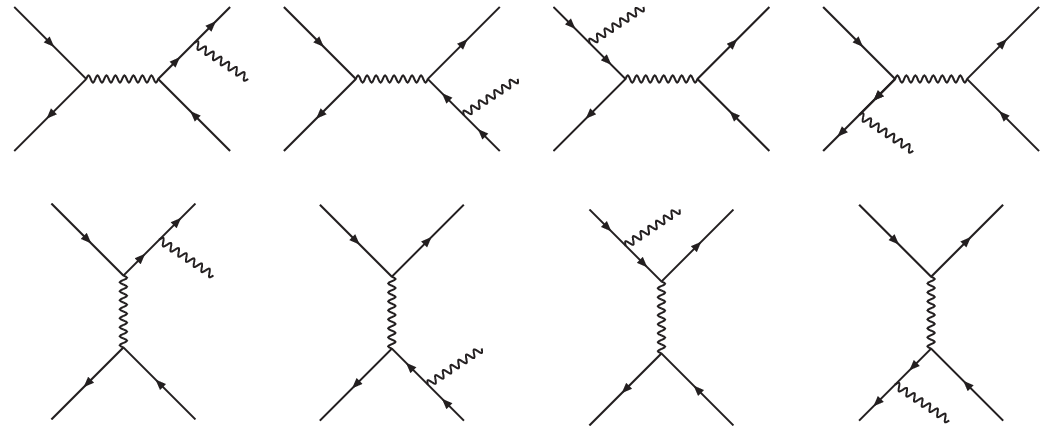
The LO cross section for real-photon emission of Eq. (1) was computed long ago in Refs. [18], and in the ultra-relativistic limit it can be written in a compact way [19]. We report its expression because it can be used for checks, although our NLO results, presented in the following sections, have been computed without any approximations, by retaining the complete dependence on the kinematical variables and keeping finite electron and muon masses. The ultra-relativistic limit of the LO results [19] are conveniently expressed in terms of the kinematic invariants of Eq. (2) and of the variables , with ,
| (5) |
where the function depends on the final-state fermions. For the process one finds
| (6) |
while for the case the function is
| (7) |
2.2 Virtual Corrections
The one-loop corrections to the two scattering processes studied in this work involve a relatively limited number of Feynman diagrams: the package QGRAF [20] generates 38 one-loop diagrams for the process and 76 diagrams for the process . Representative graphs are shown in Fig. 2; note that due to Furry’s theorem, diagrams of class 2c cancel in the sum.
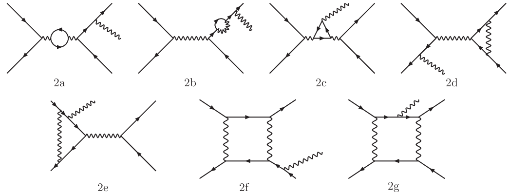
As can be seen from Fig. 2, the calculation of the complete one-loop corrections requires the evaluation of pentagon diagrams of class 2g, the most challenging and time consuming part of this calculation.
It is well known that any one-loop amplitude can be written as the sum of a linear combination of scalar box, triangle, bubble and tadpole integrals, whose analytic expressions were obtained in the seminal paper by ’t Hooft and Veltman [21], and a so-called rational part. The rational term and the coefficients multiplying the one-loop integrals are ratios of polynomials in the masses and the kinematical invariants. These coefficients have been traditionally determined by means of the Passarino-Veltman (PV) reduction method [22]. However, for processes with more than four external legs, a straightforward application of the PV reduction can generate very large expressions involving inverse Gram determinants and lead to numerical instabilities.
In recent years, a significant amount of work has been devoted to the evaluation of one-loop amplitudes for processes with five or more external legs. Besides improvements on standard techniques, where a tensor reduction is explicitly performed, new unitarity-based numerical and analytical developments have emerged (for recent reviews see Refs. [23] where an exhaustive list of references can be found). Both directions have been successfully pursued and have led to impressive results. In particular, in the last few months, very challenging calculations involving four particles in the final state, relevant for LHC phenomenology, have been completed [24, 25].
In the present letter we describe the evaluation of the one-loop corrections to the processes and , performed by means of the OPP reduction method [12, 13]. The one-loop amplitudes, generated through QGRAF, have been processed with FORM [26] routines in order to produce a FORTRAN 95 output. The latter has then been used as an input for two computer implementations of the OPP technique which numerically evaluate the coefficients of the basis integrals and the rational part for each phase-space point [27, 28]. Both codes have been interfaced with publicly available software which allows for the evaluation of the basis integrals [29, 30].
The one-loop corrections to the cross section can be written as
| (8) |
where the interference of the one-loop amplitude with the complex-conjugate tree-level amplitude is evaluated in dimensional regularization and subdivided into four contributions, according to the OPP-reduction algorithm,
| (9) |
Here denotes the cut-constructible four-dimensional part of the result, written as a linear combinations of scalar boxes, triangles, bubbles and tadpoles, stands for the so-called rational part and summarizes all contributions induced by the ultraviolet counterterms. As a technical remark, we stress that throughout our computation we have used strictly four-dimensional external momenta.
The rational part has been written through the sum of the components and , as explained in Ref. [31]. The integrand corresponding to a generic point one-loop Feynman diagram can be written as
| (10) |
where a bar denotes objects living in space-time dimensions, is the loop momentum, are linear combinations of the external four-dimensional momenta and stand for the masses of the internal legs. The numerator can be split into a four-dimensional and an -dimensional part, denoted in the following by a tilde, . The four-dimensional numerator is then expanded in terms of four-dimensional denominators [12]: the mismatch in the dimensionality between the latter and the dimensional inverse propagators of Eq. (10) generates the term in Eq. (9). The component, instead, stems from the overlap between and the ultraviolet poles of one-loop integrals, and can be evaluated in QED by employing the ad-hoc counterterm-like Feynman rules presented in Ref. [31]. Note that the overlap between the -dimensional numerator and the infrared poles of one-loop integrals can be safely neglected from the very beginning as proven in Appendix A of Ref. [32].
We carried out the ultraviolet renormalization in the on-mass-shell scheme: the renormalized charge is chosen to be equal to the value of the electromagnetic coupling, as measured in Thomson scattering, at all orders in perturbation theory; the squared fermion masses are identified with the real parts of the poles of the Dyson-resummed propagators; field-renormalization constants cancel by definition external wave-function corrections.
Throughout our computation we have retained the full dependence on the fermion masses, introducing in particular the appropriate ultraviolet and -type mass counterterm diagrams depicted in Fig. 3.

We observe that, in the limit where terms suppressed by positive powers of the electron or muon mass are neglected, the contributions induced by ultraviolet counterterms and -like rational terms can be embedded in the computation by means of simple factors multiplying the tree-level amplitude. They represent important elements for performing checks, as they can be accounted for simply by introducing counterterms at the diagrammatic level. Moreover, they can be employed for speeding up the numerical evaluation of the amplitudes in all cases where terms proportional to the fermion masses can be safely neglected.
By using the U(1) Ward identity in order to eliminate the charge counterterm, we find that the ultraviolet counterterm in Eq. (9) originates from
| (11) |
where field counterterms are defined through , , , with , and the index has been introduced for denoting renormalized quantities. Explicitly, we have the well-known expressions
where the index runs over the fermions, is the color factor ( for leptons and for quarks), is the quantum number associated with the electric charge, is the fermion mass, is the Euler-Mascheroni constant and is the ’t Hooft mass. Although QED is not simultaneously free from ultraviolet and infrared divergencies for an arbitrary number of space-time dimensions, we have followed the common practice of using the same dimensional regulator for isolating both ultraviolet and infrared poles.
Similarly, within the same approximation, the component in Eq. (9) arises from the interference of with the tree-level amplitude, where the former is defined as,
| (13) |
In both Eq. (11) and Eq. (13), vacuum polarization insertions can be easily removed by switching off all terms proportional to the sum over the fermions.
We observe that the common structure of those terms, even in the general kinematic case we worked out, suggests that the contributions to the rational term can be fully combined with ultraviolet counterterms, thus achieving a significant optimization in this part of the calculation.
The cut-constructible term and the term in Eq. (9) have been obtained by direct application of the OPP method. Here we describe the two implementations of this part of the calculation.
The first version employs the routines of the publicly available package CutTools [27] for the numerical determination of the coefficients which multiply the basis integrals. These routines have been combined with QCDLoop [29], used to evaluate the needed scalar integrals 11 1 We have used the version 1.0 of CutTools. During the completion of this work, version 1.1 has become available at http://www.ugr.es/pittau/CutTools/, with a built-in interface to QCDLoop.. The basis of loop integrals employed by CutTools involves also rank-one and rank-two two-point functions in order to improve the numerical stability respect to the case where the basis contains only scalar integrals, as described in Section 3 of Ref. [13]. The additional tensor integrals have been included coding the relations provided in Ref. [33].
The second version of the calculation is used for cross-checking our results and it makes use of an independent FORTRAN 95 code [28] for the reduction of the tensor integrals, which includes an optional optimization of the OPP technique based on the Discrete Fourier Transform [34]. The basis integrals are evaluated using the code OneLOop [30], written by A. van Hameren.
It is interesting to observe that the rational part is computed by using different strategies in the two versions of the calculation: CutTools employs the mass-shift procedure introduced in Ref. [12], while the second approach uses the counterterm-based method described in Ref. [13].
The results obtained with the two independent implementations for the cut-constructible term and the component are in very good agreement.
A final comment concerns the vacuum polarization insertions (such as diagram 2a in Fig. 2). Although these types of diagrams are implemented in both codes, they are naturally incorporated in any QED computation by simply running the fine-structure constant to the appropriate scale. Furthermore, the introduction of a running fine-structure constant allows for a straightforward inclusion of hadronic contributions using dispersion relations and the optical theorem. Since this class of corrections is well-known, it will be neglected in the rest of the paper.
2.3 Real Soft-Photon Corrections
In order to check our calculation, it is useful to control the agreement between the values of the coefficients of the residual infrared poles for the virtual one-loop corrections and those of the analytic expressions of the corresponding poles arising from real soft-photon emission diagrams. In fact, the sum of the one-loop corrections to () and the real-emission diagrams for () is infrared finite after integrating over the soft-photon phase space up to a given upper cut-off on the energy of the undetected photon .
The contribution of real soft-emission diagrams factorizes in the product of the LO cross section of Eq. (3) and an infrared-divergent coefficient which can be extracted from Ref. [35],
| (14) |
where the functions can be written in the compact form
| (15) |
with
| (16) |
and being a finite remainder which is not considered in the present work. Here we have introduced for and for . In the case , obtained by taking the limit in Eq. (15), one finds .
3 Numerical Results
In this section we show the numerical results for the squared LO amplitude, summed and averaged over the spins, and the associated one-loop virtual corrections (excluding trivial vacuum polarization insertions) for both processes at fixed phase-space points. Although the main result of our work is represented by a computer code which can eventually be interfaced with MC generators, we find it useful to show explicitly some numerical results in order to allow for detailed comparisons.
We define
| (17) |
| (18) |
where and the arbitrary ’t Hooft mass unit has been set for definiteness to the value GeV. Following Eq. (9), we further define
| (19) |
isolating the contribution of the ultraviolet counterterms from the sum of the cut-constructible and rational parts.
In the following we will show also the value of the residue the infrared pole for real soft-photon emission, introducing
| (20) |
with defined in Eq. (15).
All results have been obtained using the input data suggested by the Particle Data Book [36].
3.1 Results for
We start considering the process . We set GeV and show results for the following phase-space point:
| (21) | |||||
where and all quantities are expressed in GeV. After splitting the one-loop corrections according to Eq. (19), we obtain:
| (22) |
All results are expressed in and they have been obtained by working in double precision.
In order to check the stability of our results, we have performed the so-called test, monitoring the agreement between the numerical values of the numerator function of Eq. (10) before and after the decomposition in terms of inverse propagators [27]. When the numerical agreement in the comparison does not reach a given limit set by the user, the code automatically triggers the use of the more time-consuming multi-precision routines [37]. We observe more than 9 digits of agreement between the results obtained in double precision, requiring a relative precision for the test, and those we got after forcing multi-precision in the reduction program for reaching a relative precision.
A second test on the precision of our calculation concerns the cancellation of the poles. After renormalization, the residual pole for is of pure infrared origin and it matches the infrared pole in with an agreement of 9 digits.
Finally, as stressed in Section 2.2, we have performed the calculation of all contributions by means of two independent codes.
As a further test of the stability of our results, we study the process for configurations in which the muon, or the antimuon, is (almost) parallel to the emitted photon. We set GeV and fix the momenta of the colliding leptons and the outgoing photon to be:
| (23) | |||||
with all momenta given in GeV.

Then, we calculate the finite part of the virtual corrections of Eq. (18), as a function of the energy of the outgoing muon : the results are illustrated in Fig. 4. On the left side of the plot, for low values of , we are in a configuration in which the muon is almost parallel to the photon, while the antimuon goes in the opposite direction; we then progressively rotate the muon, keeping the four-momentum of the photon fixed, until the muon becomes anti-parallel to the photon, while the antimuon becomes almost parallel to it. While we observe the appearance of collinear divergencies, the virtual corrections follow a smooth curve, thus suggesting a good stability of our result even in this particular kinematic configuration.
3.2 Results for
Here we consider the process . We set GeV and present numerical results for the following phase-space point:
| (24) | |||||
with all quantities expressed in GeV. We obtain
| (25) |
where all results are expressed in .
All the numbers have been obtained by working in double precision and requiring a relative precision for the test. Also for this process, we have tested the precision of our calculation by forcing multi-precision in the reduction program, by checking the complete cancellation of ultraviolet and infrared poles and by comparing the two independent implementations.
Following the same idea of Fig. 4, we plot in Fig. 5 the finite part of the virtual corrections, of Eq. (18), as a function of the energy of the outgoing electron , ranging between two configurations where the electron momentum is (almost) parallel or anti-parallel to the photon momentum and collinear divergencies show up.

4 Conclusions
We have applied the OPP method to evaluate the complete NLO virtual QED corrections to the hard bremsstrahlung processes and , both relevant for determining the luminosity at low-energy electron-positron colliders.
It is interesting to note that in the case of muon-pair production in association with a hard photon the calculation has been performed retaining both the electron and muon masses. This shows the capability of the method in dealing with several scales inside the loop diagrams.
The numerical stability of the results has been tested by means of three different procedures: the check on the quality of the reconstructed numerators given by the test; the comparison of infrared divergencies arising from virtual and real corrections, which cancel as they should; the agreement of the results obtained using two independent codes. In particular, for LO calculations, we find an agreement of at least 12 digits; for NLO results, we have 9 digits of accuracy.
The main result of our calculation is the implementation of hard-bremsstrahlung emission corrections, both for Bhabha scattering and muon-pair production, into a FORTRAN 95 code which employs the publicly available package CutTools for the extraction of the coefficients of the scalar integrals and the package QCDLoop for evaluating the needed scalar integrals.
The typical order of magnitude of the CPU time of the FORTRAN 95 code we have developed is seconds for each phase-space point on a standard desktop machine. The computational speed, together with the modular approach we have followed in computing the radiative corrections, allows for an implementation of the results in the existing MC programs.
Once supplemented with the finite part for real-emission diagrams, the results we have derived allow for a phenomenological study of the two hard-bremsstrahlung processes and , including the calculation of the cross sections and the relevant distributions. In addition, they can be compared with the corrections already implemented in MC generators in order to assess the associated theoretical uncertainty.
Acknowledgments
We thank Andrea Ferroglia for his invaluable help during all stages of the computation. We also thank Stefano Pozzorini for discussions and clarifications concerning the interplay between infrared poles and rational terms, R. Keith Ellis and Giulia Zanderighi for useful communications concerning QCDLoop and André van Hameren for help with OneLOop. Feynman diagrams have been drawn with the packages Axodraw [38] and Jaxodraw [39].
The research of S.A. was supported by the Deutsche Forschungsgemeinschaft through Sonderforschungsbereich Transregio 9 Computergestützte Theoretische Teilchenphysik, and in part by the BMBF through the Nutzungsinitiative CERN. The work of G.O. was supported in part by the NSF Grant No. PHY-0855489. S.A. and G.O. gratefully acknowledge the hospitality of CERN at various stages of this work.
References
- [1]
C.M. Carloni Calame, C. Lunardini, G. Montagna, O. Nicrosini and F. Piccinini,
Nucl. Phys. B 584 (2000) 459, arXiv:hep-ph/0003268;
C.M. Carloni Calame, Phys. Lett. B 520 (2001) 16, arXiv:hep-ph/0103117;
G. Balossini, C.M. Carloni Calame, G. Montagna, O. Nicrosini and F. Piccinini, Nucl. Phys. B 758 (2006) 227, arXiv:hep-ph/0607181. - [2]
A.B. Arbuzov, G.V. Fedotovich, E.A. Kuraev, N.P. Merenkov, V.D. Rushai and L. Trentadue,
JHEP 9710 (1997) 001, arXiv:hep-ph/9702262;
A.B. Arbuzov, G.V. Fedotovich, F.V. Ignatov, E.A. Kuraev and A.L. Sibidanov, Eur. Phys. J. C 46 (2006) 689, arXiv:hep-ph/0504233. - [3] S. Jadach, W. Placzek and B.F.L. Ward, Phys. Lett. B 390 (1997) 298, arXiv:hep-ph/9608412.
- [4] G. Balossini, C. Bignamini, C.M. Carloni Calame, G. Montagna, O. Nicrosini and F. Piccinini, Nucl. Phys. Proc. Suppl. 183 (2008) 168, arXiv:0806.4909 [hep-ph].
- [5]
M. Consoli,
Nucl. Phys. B 160 (1979) 208;
M. Böhm, A. Denner, W. Hollik and R. Sommer, Phys. Lett. B 144 (1984) 414. - [6] R. Bonciani, A. Ferroglia, P. Mastrolia, E. Remiddi and J.J. van der Bij, Nucl. Phys. B 701 (2004) 121, arXiv:hep-ph/0405275; Nucl. Phys. B 716 (2005) 280, arXiv:hep-ph/0411321.
- [7]
A.A. Penin,
Phys. Rev. Lett. 95 (2005) 010408, arXiv:hep-ph/0501120;
Nucl. Phys. B 734 (2006) 185, arXiv:hep-ph/0508127;
R. Bonciani and A. Ferroglia, Phys. Rev. D 72 (2005) 056004, arXiv:hep-ph/0507047. - [8]
T. Becher and K. Melnikov,
JHEP 0706 (2007) 084, arXiv:0704.3582 [hep-ph];
S. Actis, M. Czakon, J. Gluza and T. Riemann, Nucl. Phys. B 786 (2007) 26, arXiv:0704.2400 [hep-ph]. - [9]
S. Actis, M. Czakon, J. Gluza and T. Riemann,
Phys. Rev. Lett. 100 (2008) 131602, arXiv:0711.3847 [hep-ph];
Phys. Rev. D 78 (2008) 085019, arXiv:0807.4691 [hep-ph];
R. Bonciani, A. Ferroglia and A.A. Penin, Phys. Rev. Lett. 100 (2008) 131601, arXiv:0710.4775 [hep-ph]; JHEP 0802 (2008) 080, arXiv:0802.2215 [hep-ph];
J.H. Kühn and S. Uccirati, Nucl. Phys. B 806 (2009) 300, arXiv:0807.1284 [hep-ph]. - [10]
A.B. Arbuzov, V.S. Fadin, E.A. Kuraev, L.N. Lipatov, N.P. Merenkov and L. Trentadue,
Nucl. Phys. B 485 (1997) 457, arXiv:hep-ph/9512344;
S. Jadach, M. Melles, B.F.L. Ward and S.A. Yost, Phys. Lett. B 377 (1996) 168, arXiv:hep-ph/9603248;
B.F.L. Ward, S. Jadach, M. Melles and S.A. Yost, Phys. Lett. B 450 (1999) 262, arXiv:hep-ph/9811245. - [11]
S. Jadach, M. Melles, B.F.L. Ward and S.A. Yost,
Phys. Rev. D 65 (2002) 073030, arXiv:hep-ph/0109279;
H. Czy, A. Grzelinska, J.H. Kühn and G. Rodrigo, Eur. Phys. J. C 33 (2004) 333, arXiv:hep-ph/0308312. - [12] G. Ossola, C.G. Papadopoulos and R. Pittau, Nucl. Phys. B 763 (2007) 147, arXiv:hep-ph/0609007.
- [13] G. Ossola, C.G. Papadopoulos and R. Pittau, JHEP 0707 (2007) 085, arXiv:0704.1271 [hep-ph].
- [14] F. del Aguila and R. Pittau, JHEP 0407 (2004) 017, arXiv:hep-ph/0404120.
- [15] H. Czy, A. Grzelinska, J.H. Kühn and G. Rodrigo, Eur. Phys. J. C 39 (2005) 411, arXiv:hep-ph/0404078.
- [16] S. Jadach, B.F.L. Ward and Z. Was, Comput. Phys. Commun. 130 (2000) 260, arXiv:hep-ph/9912214; Phys. Rev. D 63 (2001) 113009, arXiv:hep-ph/0006359.
- [17] S. Jadach, B.F.L. Ward and S.A. Yost, Phys. Rev. D 73 (2006) 073001, arXiv:hep-ph/0602197.
- [18]
S.M. Swanson,
Phys. Rev. 154 (1967) 1601;
A.C. Hearn, P.K. Kuo and D.R. Yennie, Phys. Rev. 187 (1969) 1950. - [19] F.A. Berends, R. Kleiss, P. De Causmaecker, R. Gastmans and T.T. Wu, Phys. Lett. B 103 (1981) 124.
- [20] P. Nogueira, J. Comput. Phys. 105 (1993) 279.
- [21] G. ’t Hooft and M.J.G. Veltman, Nucl. Phys. B 153 (1979) 365.
- [22] G. Passarino and M.J.G. Veltman, Nucl. Phys. B 160 (1979) 151.
- [23]
Z. Bern et al.,
summary report of the NLO multileg working group of the Les Houches
2007 workshop Physics at TeV Colliders,
arXiv:0803.0494 [hep-ph];
T. Binoth, PoS ACAT08 (2008) 011, arXiv:0903.1876 [hep-ph]. - [24]
A. Bredenstein, A. Denner, S. Dittmaier and S. Pozzorini,
Phys. Rev. Lett. 103 (2009) 012002,
arXiv:0905.0110 [hep-ph];
G. Bevilacqua, M. Czakon, C.G. Papadopoulos, R. Pittau and M. Worek, arXiv:0907.4723 [hep-ph]. - [25]
R.K. Ellis, K. Melnikov and G. Zanderighi,
arXiv:0906.1445 [hep-ph];
C.F. Berger, Z. Bern, L.J. Dixon, F. Febres Cordero, D. Forde, T. Gleisberg, H. Ita, D.A. Kosower and D. Maitre, arXiv:0907.1984 [hep-ph]. - [26] J.A.M. Vermaseren, New Features of FORM, arXiv:math-ph/0010025.
- [27] G. Ossola, C.G. Papadopoulos and R. Pittau, JHEP 0803 (2008) 042, arXiv:0711.3596 [hep-ph].
- [28] Red, unpublished.
- [29]
R.K. Ellis and G. Zanderighi,
JHEP 0802 (2008) 002, arXiv:0712.1851 [hep-ph];
G.J. van Oldenborgh, Comput. Phys. Commun. 66 (1991) 1. - [30]
A. van Hameren, C.G. Papadopoulos and R. Pittau,
arXiv:0903.4665 [hep-ph];
A. van Hameren, J. Vollinga and S. Weinzierl, Eur. Phys. J. C 41 (2005) 361, arXiv:hep-ph/0502165. - [31] G. Ossola, C.G. Papadopoulos and R. Pittau, JHEP 0805 (2008) 004, arXiv:0802.1876 [hep-ph].
- [32] A. Bredenstein, A. Denner, S. Dittmaier and S. Pozzorini, JHEP 0808 (2008) 108, arXiv:0807.1248 [hep-ph].
- [33] A. Denner and S. Dittmaier, Nucl. Phys. B 734 (2006) 62, arXiv:hep-ph/0509141.
- [34] P. Mastrolia, G. Ossola, C.G. Papadopoulos and R. Pittau, JHEP 0806 (2008) 030, arXiv:0803.3964 [hep-ph].
- [35] D.Y. Bardin and G. Passarino, The Standard Model in the Making, Oxford University Press, 1999.
- [36] C. Amsler et al. (Particle Data Group), Phys. Lett. B 667 (2008) 1.
- [37] D.H. Bailey, ACM Transactions on Mathematical Software, vol. 21, no.4 (1995) 379.
- [38] J.A.M. Vermaseren, Comput. Phys. Commun. 83 (1994) 45.
- [39] D. Binosi and L. Theussl, Comput. Phys. Commun. 161 (2004) 76, hep-ph/0309015.