Small-world behavior in time-varying graphs
Abstract
Connections in complex networks are inherently fluctuating over time and exhibit more dimensionality than analysis based on standard static graph measures can capture. Here, we introduce the concepts of temporal paths and distance in time-varying graphs. We define as temporal small world a time-varying graph in which the links are highly clustered in time, yet the nodes are at small average temporal distances. We explore the small-world behavior in synthetic time-varying networks of mobile agents, and in real social and biological time-varying systems.
pacs
89.75.-k, 89.75.Hc, 89.75.Fb, 87.19.ljIn the last decade, the study of complex networks has attracted a lot of attention in the scientific community as various social, biological and technological systems can be represented and analysed as graphs [1]. Typically, such systems are inherently dynamic, with the links changing and fluctuating over time. Human contacts or relationships change over time because individuals lose old acquaintances, acquire new ones, or move over geographic space [2, 3]. Communication in man-made networks, such as machine connections and social interactions over the Internet, takes place at specific points in time [4, 5, 6]. New links appear while some others disappear in the World-Wide-Web [7], in patterns of interactions among gene from microarray time experiments [8, 9] or in functional brain networks [10, 11]. The time evolution of a network by the addition, as well as the deletion, of nodes and links has been extensively modelled with the main purpose of reproducing, asymptotically, statistical properties such as scale-free degree distributions [1, 12]. With only a few notable exceptions [13, 14, 15], less focus has been given to the characterization of the dynamics of complex networks in stationary conditions.
In particular, the small-world phenomenon, i.e., the fact that real networks have high clustering coefficient, while the typical distance between their nodes is small as in random graphs, has been investigated in static graphs, neglecting the temporal dimension [16, 17, 18]. The time evolution of a real system, when considered, is usually studied by evaluating the standard static measures (distances and clustering coefficient) on snapshots of the network taken at different times [19, 20]. As we will show below, this approach does not capture entirely the dynamic correlations of a time-varying network. In this Letter, we introduce a measure of the temporal distance between the nodes of time-varying graphs, i.e. graphs with time-fluctuating links. Such temporal distance takes into account the actual time order, duration and correlations between links appearing at different times. This metric, together with a measure of the time-persistence of the links, allows to define and investigate temporal small-world behavior in social and biological networks that change over time.
Consider a network with nodes, where the links can fluctuate in time. The typical example is a social system, with no births or deaths, where the patterns of interaction are changing in time because of the spatial movement of the individuals, or because the individuals lose old acquaintances and get new ones. The system can be described at its maximum resolution sampling time as a time-varying graph, i.e. a discrete sequence (an ordered set) of undirected or directed graphs, where is the length of the sequence. In compact notation, we denote the entire sequence as . A time-varying graph can be represented by means of a time-dependent adjacency matrix , where are the elements of the adjacency matrix of the -th graph. We indicate as the number of links in the -th graph of the sequence. A sequence of graphs is convenient to describe systems where each connection starts at a specific time, and also has a temporal duration. In this sense, time-varying graphs are different from previous temporal approaches [4, 5, 21, 22] designed to characterize systems as email exchanges, where the links have instead no temporal duration, because the exchange is instantaneous. Moreover, a time-varying graph is a different ensemble from those usually studied in the literature [23, 24]. In fact, in a time-varying graph, what matters is not only the probabilty distribution over the graphs in the ensemble, but also how the graphs are ordered in time. By counting the number of times a given graph appears in the time sequence, we can construct . To fully describe time-varying graphs we also need to know how graphs are correlated in time. For instance we need to know the conditional probabilities of observing graph after graph (more in general, the probabilities of observing graph after the sequence ). In most cases, the contacts between the same node pair in time-varying systems tend to be clustered in time, i.e. they show persistence over time [4]. For instance, people tend to engage in relations for continuous intervals of time. Hence, a given link has a higher probability to appear in graph if it was already present in graph . To quantify this effect, following Ref. [20] we compute , the average topological overlap of the neighbor set of a node between two successive graphs in the sequence:
| (1) |
We name this metric the temporal-correlation coefficient of . The value of C is in the range [0,1]. In particular, if all graphs in the sequence are equal, we have .
A fundamental concept in graph theory is that of geodesic, or shortest path. In a static graph, a shortest path between nodes and is defined as a path of minimal length between the two nodes. This is a sequence of adjacent nodes starting at , ending at , and visiting the minimum number of nodes. Finally, the distance between node and node is set equal to the length of the shortest paths from to . Here, we introduce the concepts of temporal shortest path and temporal distance to generalize the definitions of shortest paths and of node distance to the case of time-varying graphs. We illustrate the basic idea with the example shown in Fig. 1a. Suppose node wants to send a message in the fastest possible way to the other nodes of the graph. We assume that node can start passing the message at time , and the message has to be delivered by time . On graph , node can directly pass the message to nodes and , which are therefore assigned temporal distance 1 from node , since they can be reached in one unit of time. There are also other temporal paths to go from to nodes and in three time units. For example, we can go from to in the following way: in , in . This is also a temporal path from to , though it is not the shortest, since the fastest way to go from to is to use the link in . Distance 3 is assigned to node , since the message can be passed from to in graph , and then from node to node in , thus reaching in three time units.
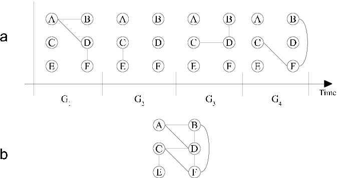
Node can be reached in 4 time steps by means of three alternative shortest paths: in , in ; in , in , in ; and in , in , in . Finally, there are no temporal paths from to , hence we set the temporal distance of from equal to , and we say that is not reachable from . This is an effect of the time order of the links in a time-varying graph, and indeed node and are connected in the aggregate graph shown in Fig. 1b in which all links are considered as concurrent.
Notice also that, due to the time order of the links, the temporal distances are not symmetric, even if the time-varying graph consists of a sequence of undirected graphs. For instance, while the temporal distance from to is 4, the temporal distance from to is (because the links occur in the wrong time order to facilitate the passage from to ). Conversely, in the static graph in Fig. 1b, we have . In order words, the main difference between a time-varying graph G, as that shown in panel a), and its associated static graph, reported in panel b), is that some of the shortest paths of the static graph are not temporally valid (in the sense that the links do not appear in the correct time order) and, therefore, cannot be used to route messages. In general, in time-varying graphs there are more disconnected node pairs, than in static ones. As an example, the static graph in Fig. 1 is composed of a single connected component, while if time is taken into consideration, it is not possible to go from to , or from to . In order to compute the temporal distances for all node pairs of a generic graph , we have implemented a generalization of the breadth first search algorithm. The average temporal connectivity properties of can be measured by the characteristic temporal path length :
| (2) |
Alternatively, in order to avoid the potential divergence due to pairs of nodes that are not temporally connected, we can define the temporal global efficiency of as [17]:
| (3) |
Low values of (high values of ) indicate that the nodes of the graphs can communicate efficiently. In the following, we will show that time-varying graphs from models and real-world systems can be, at the same time, temporally clustered and still have small temporal distances between their nodes. In analogy with the small-world analysis in static graphs [16, 17], we will compare the actual values of , and of a given time-varying graph , with the corresponding values calculated by considering an ensemble of randomized versions of . Each sequence is obtained by randomly reshuffling the graphs in , i.e., by destroying the time order (and correlations) in the original sequence . More precisely, we will show that some time-varying graphs can have a value of much larger than the correlation coefficient of the reshuffled sequence , and, at the same time a value of as small as . We will refer to this behavior as small-world behavior in time-varying systems.

Random-walkers network model.- We first illustrate how this behavior can be obtained in a network model of moving agents, as a result of simple motion rules. We consider a system of random walkers which move in a two-dimensional square of linear size with a fixed velocity , and additionally perform long-distance jumps to randomly chosen position of the square with a jump probability [3]. For each fixed value of , the time-varying network is constructed by linking, every second, all nodes having a distance in space smaller than a given value . In Fig. 2 we plot and as a function of . The values reported are normalized to the maximum values of and obtained for , and respectively equal to and . We observe that a small percentage of jumps is sufficient to create links between nodes otherwise at large temporal distances and to produce a large drop in the temporal . When , has reduced to one forth of , and when , has about the same value as for the reshuffled sequence. The value of obtained as an average over 1000 realizations of is reported as dashed line. While is rapidly decreasing, is constant up to large values of , so that for intermediate values of we have time-varying graphs exibiting small-world behavior. Finally, we have found that, by approximating for each value of the corresponding time-varying graph as a static graph, we obtain a value of static L (not reported in figure) which slowly changes in the interval . For instance, for , we have . We thus cannot capture the temporal small-world behavior with the standard characteristic path length of a static graph.
Brain cortical networks.- We finally explore real-world time-varying complex networks. We first consider time-varying functional cortical networks extracted from a set of high-resolution EEG recordings in a group of 5 normal subjects performing a task consisting in a foot movement [11]. For each subject, and for each of four frequency bands (), we considered a time period of 0.5 sec corresponding to the final phase of execution of the foot movement. Each time-varying graph has nodes, representing cortical regions of interest, and consists in a time sequence of directed unweighted graphs, where the directed links represent causal influences between cortical regions (see Ref. [11] for details).
| 0.44 | 0.18 (0.03) | 3.9 | 4.2 | 0.50 | 0.48 | |
| 0.40 | 0.17 (0.002) | 6.0 | 3.6 | 0.41 | 0.45 | |
| 0.48 | 0.13 (0.003) | 12.2 | 8.7 | 0.39 | 0.37 | |
| 0.44 | 0.17 (0.003) | 2.2 | 2.4 | 0.57 | 0.56 | |
| d1 | 0.80 | 0.44 (0.01) | 8.84 | 6.00 | 0.192 | 0.209 |
| d2 | 0.78 | 0.35 (0.01) | 5.04 | 4.01 | 0.293 | 0.298 |
| d3 | 0.81 | 0.38 (0.01) | 9.06 | 6.76 | 0.134 | 0.141 |
| d4 | 0.83 | 0.39 (0.01) | 21.42 | 15.55 | 0.019 | 0.028 |
| Mar | 0.044 | 0.007 (0.0002) | 456 | 451 | 0.000183 | 0.000210 |
| Jun | 0.046 | 0.006 (0.0002) | 380 | 361 | 0.000047 | 0.000057 |
| Sep | 0.046 | 0.006 (0.0002) | 414 | 415 | 0.000058 | 0.000074 |
| Dec | 0.049 | 0.006 (0.0002) | 403 | 395 | 0.000047 | 0.000059 |
We have computed the values of , and for each real sequence and for the reshuffled ones. In Table 1 we report the results for one of the subjects. For all the considered bands, the real sequence exhibits small-world properties, having a large value of (significantly larger than ) and, at the same time, a small characteristic temporal path length (a high efficiency), comparable to that observed in the shuffled sequence. Similar results (not reported) were obtained for the other four subjects.
Social interaction networks.- The second real case study of our analysis is a time-varying social network based on a dataset of contacts among participants of INFOCOM’06, a major data communication conference which took place in a hotel. The contacts were collected by means of Bluetooth-enabled devices able to record interactions among people that are in promixity [26]. The discovery process of new devices was performed every 2 minutes. In Table 1 we report the data for the interactions during lunchtime between 1pm and 2:30pm. This is the interval with the larger number of contacts during a day. Each sequence is made of undirected unweighted graphs with nodes each. The average path length and the efficiency are similar for the original and reshuffled traces (the number in parenthesis close to and are the percentage of pair of nodes being temporally connected and hence considered in the computation of the average path length), whereas is more than double that of . This can be considered as an indication of small-world behavior in these traces according to our definition.
Online social networks.- The third system we study is based on interactions over an online social network. The original dataset contains the messages sent among 6 millions users in the London network of Facebook over one year (March 2007 to February 2008) [27]. We have divided the contacts according to the months of the year and, for each month, we have filtered out all contacts between pairs of nodes which exchange less than 10 messages per month. This allows us to consider only the subset of most active users, obtaining networks with about users per month. For each month, the time varying graph is composed by (or ) directed graphs, one for each hour of the month. As shown in Table 1 for four different months of the dataset, the average temporal path length of the time-varying networks is close to the value obtained for the reshuffled sequences. However, the network under study is disconnected in several different components, and only an extremely small percentage (about ) of the node couples are temporally connected. Consequently, the characteristic temporal path length was evaluated as an average over a small number of node couples. A better characterization of the system can be obtained by means of the temporal efficiency. The values of and measured for Facebook are in general smaller than those observed in the other two networks, this being due to the high disconnectedness of Facebook. Nevertheless, as for the case of the cortical networks and of INFOCOM’06, the real Facebook is almost as efficient as its reshuffled version. Finally, also for Facebook we observe a temporal small-world behavior: while the length of the temporal paths of the time-varying network are not affected by the reshuffling procedure, the temporal correlation coefficient is about one order of magnitude larger than in the reshuffled version .
In conclusion, our results suggest that time-varying networks, strongly clustered in time and, at the same time, with short temporal paths between their nodes, might be widespread in biological, social and man-made systems, often with important dynamical consequences [25]. We hope that our work will stimulate further studies of temporal small-world behavior in real time-varying systems.
We thank F. Babiloni and F. De Vico Fallani for making the cortical networks available to us, and Ben Y. Zhao (UCSB) for the Facebook traces. We acknowledge the support of EPSRC through grants EP/C544773, EP/E012914 and EP/D077273.
References
- [1] R. Albert and A.-L. Barabási, Rev. Mod. Phys. 74, 47 (2002); S.N. Dorogovtesev, J.F.F. Mendes, Evolution of networks,(Oxford University Press, 2003); S. Boccaletti, et al., Phys. Rep. 424, 175 (2006).
- [2] M. C. González, C.A. Hidalgo and A.-L. Barabási, Nature 453, 779 (2008).
- [3] A. Buscarino, L. Fortuna, M. Frasca, V. Latora, Europhys. Lett. 82, 38002 (2008).
- [4] P. Holme, Phys. Rev. E 71, 046119 (2005).
- [5] G. Kossinets, J. Kleinberg, and D. Watts, arXiv:0806.3201 (2008).
- [6] B. Tadić and S. Thurner, Physica A 332, 566 (2004)
- [7] B. Tadić, Physica A 293, 273 (2001)
- [8] C. Caretta-Cartozo, P. De Los Rios, F. Piazza, P. Liò, PLoS Computational Biology, 3, e103 (2007).
- [9] A. Ahmed and E. P. Xing, Proc. Natl. Acad. Sci. USA 106, 11878 (2009).
- [10] M. Valencia, J. Martinerie, S. Dupont, and M. Chavez, Phys. Rev. E. 77, 050905R (2008).
- [11] F. De Vico Fallani et al., Journ. Phys. A: Math. Theor. 41, 224014 (2008)
- [12] S.N. Dorogovtsev and J.F.F. Mendes, Phys. Rev. E 63, 056125 (2001).
- [13] A. Gautreau, A. Barrat, and M. Barthelemy, Proc. Nat. Acad. Sci., 106, 8847 (2009).
- [14] A. Raval, Phys. Rev. E 68, 066119 (2003).
- [15] J. Stehle, A. Barrat, G. Bianconi, arXiv:1002.4109
- [16] D. J. Watts and S. H. Strogatz, Nature 393, 440 (1998).
- [17] V. Latora and M. Marchiori, Phys. Rev. Lett. 87, 198701 (2001).
- [18] C. Caretta Cartozo and P. De Los Rios Phys. Rev. Lett. 102, 238703 (2009).
- [19] A.-L. Barabási, H. Jeong, R. Ravasz, Z. Neda, T. Vicsek, and A. Schubert, Physica A 311, 590 (2002).
- [20] A. Clauset and N. Eagle. Persistence and Periodicity in a Dynamic Proximity Network. In Proc. of DIMACS Workshop on Computational Methods for Dynamic Interaction Network, 2007.
- [21] D. Kempe, J. Kleinberg, and A. Kumar, J. Comp. Sys. Sci., 64, 820 (2002).
- [22] V. Kostakos, Physica A 388, 1007 (2009).
- [23] J. Park, M. E. J. Newman, Phys. Rev. E 70, 066117 (2004)
- [24] G. Bianconi Phys. Rev. E. 79, 036114 (2009).
- [25] In our discussion, we have implicitly assumed that the typical time, , to pass a message from a node to one of its first neighbors, is of the same order as the typical time, , at which the graphs in the sequence are changing. We can simulate the case by increasing the reach of a message (within a graph in the sequence) past its first neighbors. Note however that as the reach increases, the values of L will decrease while C does not change; therefore our main results still hold.
- [26] J. Scott, R. Gass, J. Crowcroft, P. Hui, C. Diot, and A. Chaintreau, CRAWDAD Trace, Infocom2006.
- [27] C. Wilson, B. Boe, A. Sala, K.P.N. Puttaswamy, and B.Y.Zhao, Procs. of EuroSys ’09, pp. 205–218 (2009)