Multi-Calorons Revisited
Atsushi Nakamula11 1 e-mail: nakamula@sci.kitasato-u.ac.jp and Jun Sakaguchi22 2 e-mail: jsakaguchi@sci.kitasato-u.ac.jp
Department of Physics, School of Science
Kitasato University,
Sagamihara, 228-8555, Japan
Abstract
Analytic Nahm data is re-examined for calorons, or periodic instantons, of instanton charge . The Nahm equations are solved analytically in terms of Jacobi elliptic functions and the possible matching conditions are classified. The dimensions of framed moduli space for charge caloron is enumerated and the maximal parameter, which is for charge , case is identified. The monopole and instanton limits are also considered. It is found that the Nahm data which does not correspond to the standard monopoles plays significant role for calorons.
1 Introduction
Calorons are finite-action ASD (anti-self-dual) solutions of Yang-Mills gauge theories on partially compactified space . We can interpret them as not only periodic instantons around the direction, but also the composite objects of constituent “monopoles”. The latter interpretation is due to the fact that calorons can be seen as the monopoles of loop group gauge theories [1, 2]. Accordingly, they have the charges of both instanton and monopole.
On analytic solutions of calorons, there has been found solutions with trivial holonomy in late 1970’s [3] by ansatz. A special class of periodic instantons are also found in [4]. In 1980’s, Nahm formulated a systematic device to construct calorons, as well as monopoles, by applying the ADHM construction of instantons [5], i.e., the Nahm construction [6]. In this formulation, caloron gauge connections can be obtained by solving one-dimensional Weyl equations on finite intervals with “impurities” at the boundaries. The dual gauge connection in Weyl operators, along with the impurities, are called Nahm data, which gives the moduli space of calorons. The dual transformation between the Nahm data and the caloron gauge connections is called the Nahm transform, which plays crucial role in the Nahm construction. The bijection between the Nahm data and the calorons has been considered earlier in [7], and proved in [8].
For a long time, calorons have been attracted much attention from various field of mathematical physics. In gauge theories, particularly important topic on calorons is that they are considered to be explaining the confinement phase in finite temperature QCD. Although calorons are thought to be ineffective for such non-perturbative effects in early days [9], the discovery of the calorons with non-trivial holonomy [10, 11], at the end of the last century, changes situation drastically. They are currently believed to play a fundamental role for the confinement. In this context, the characteristic properties of calorons, e.g., action densities, quantum corrections [12, 13, 14] and so on, are vigorously studied for gauge group.
Another interest on calorons comes from the string-theoretical point of view, where a dual transformation of D-branes leads to the Nahm construction of calorons, i.e., the D-brane interpretation [15, 16, 17]. Recent development of this field provides further interest on the instanton moduli space on ALF (asymptotically locally flat) hyper-Kähler four-manifolds [18, 19], such as multi-centered Taub-NUT spaces. Since the trivial, or flat, ALF space is , exhaustive analysis of caloron moduli space will give further insight into the instanton moduli space on non-flat ALF spaces.
On the analysis of the caloron moduli space, it has been shown that the Nahm data of calorons are an open subset of that of instantons [20], and that the dimensions of the framed moduli space to calorons are [21], where is an instanton charge. Although the formal structure of the caloron moduli space is examined in this way, the explicit descriptions of the Nahm data, particularly for higher charge cases, are studied in quite restricted cases due to analytical difficulty.
In this paper, we investigate the explicit parameterizations to the Nahm data for calorons of instanton charge in detail, though the “general” Nahm data have been appeared already in [20, 22, 23]. We make a re-construction of the Nahm data in their appropriate form to overview the caloron moduli space , and find that they include the Nahm data of parameters, which is maximal, i.e., .
We also consider the interrelation between calorons and monopoles or instantons, respectively. It is naively believed that the large instanton scale limit of calorons gives BPS monopoles in , while the large period limit gives instantons in . In this context, it has been shown that there actually exist those limiting cases in the calorons with special symmetry [24]. However, it is known that even for the calorons of with trivial holonomy do not have a monopole limit [25]. Thus, a natural question arises that which conditions on calorons admit the monopole limit. In this paper, we also give the examples of calorons which have monopole or instanton limit.
This paper is organized as follows. In section 2, we make an overview of the Nahm transform for calorons. In section 3, we give the exact Nahm data of two-calorons in their appropriate form to count the moduli space dimensions. In section 4, we give the moduli space dimensions for the two-calorons obtained in section 3, which include the maximal parameter cases. In section 5, we consider the large scale and the large period limit of the calorons obtained so far. Section 6 is devoted to concluding remarks.
2 Nahm transform for calorons
2.1 Nahm data of calorons
One of the characteristic charge of calorons is the instanton charge . As mentioned in introduction, calorons can be interpreted as a composite object of “constituent monopoles”. In gauge theory, the constituent monopoles are composed of -set of multi-monopoles. In this paper, we restrict ourselves to consider calorons of gauge group without net magnetic charge. Of this type of calorons, the two-set of multi-monopoles have an equal and opposite magnetic charges. We occasionally denote the charge -calorons without net magnetic charge as charge -calorons.
Another significant quantity for calorons is the masses of constituent monopoles, , where and are defined shortly. Note that the order of the constituent monopoles is not crucial, because there is a large gauge transformation which exchange this order, the rotation map. The asymptotic form of the gauge potential for calorons is characterized by these caloron charges and the net magnetic charge , as
| (2.1) |
We consider only the case as mentioned above.
The caloron Nahm data consists of two parts. One of them is the bulk Nahm data, and the other is the boundary data. The bulk Nahm data is four hermitian matrices , which are analytic and periodic in with periodicity , and defined on the fundamental interval . The fundamental interval is composed of two parts, . We denote the four matrices on and on , respectively. Note that the definition of the fundamental interval and its decomposition are equivalent to , and and , by the periodicity.
For the gauge field to be anti-self-dual, the matrices must enjoy the Nahm equations on each interval,
| (2.2) |
where or , and the roman subscripts are or . They also have to satisfy the reality conditions
| (2.3) |
where the periodicity is taken into account.
The boundary Nahm data are a -row vector with quaternion element, and quaternion projection matrices
| (2.4) |
where is a pure imaginary unit quaternion, namely, . Here the definition of the quaternion element is
| (2.5) |
They give the matching conditions for the bulk Nahm data at , such as
| (2.6a) | |||
| (2.6b) | |||
for the -calorons, where or . In the right-hand-side of (2.6), the trace is for quaternions so that they give a matrix.
For later purpose, we show the exact form of the right-hand-side of (2.6) for , which can be expressed in terms of the standard basis. Let us take with two quaternions and , whose components are and . Then we find
| (2.7) |
where the coefficients of basis are
| (2.8a) | |||||
| (2.8b) | |||||
| (2.8c) | |||||
| (2.8d) | |||||
2.2 Nahm transform
As is well known, a caloron gauge field is obtained from the Nahm data through the Nahm transform. The procedure of the Nahm transform for the calorons is as follows. Firstly, we solve the “Weyl equation” for -column “spinor” with quaternion entries defined on each interval and ,
| (2.9) |
where . Next, we find out a quaternion enjoying the matching conditions
| (2.10a) | |||
| (2.10b) | |||
In addition, and should be normalized as
| (2.11) |
By using these “parts”, the gauge potential is given by
| (2.12) |
2.3 Gauge transformation to Nahm data
There exist continuous transformations for the Nahm data which preserve the gauge potential (2.12). One of them is generated by a valued smooth function defined on , enjoying reality condition . The action on the Nahm data is
| (2.13a) | |||
| (2.13b) | |||
| (2.13c) | |||
Simultaneously, the Weyl spinor transforms as
| (2.14) |
with unchanged.
There is another transformation generated by a unit quaternion which preserves (2.12). It acts on the Nahm data as
| (2.15a) | |||
| (2.15b) | |||
and
| (2.16) |
We call these two types of transformation as the gauge transformation for the Nahm data.
3 Exact Nahm data of two-calorons
In this section, we will find the analytic Nahm data of caloron in its appropriate form for later consideration.
3.1 Bulk solutions
First, we have to solve the bulk equations (2.2) in both intervals and , independently. We take the following form for the matrices by using the standard basis,
| (3.1a) | |||||
| (3.1b) | |||||
| (3.1c) | |||||
where is a cyclic permutation of , , and are functions on each interval. In addition, we assume , where is a constant to be a moduli parameter. From (3.1), the Nahm equations (2.2) are
| (3.2a) | |||
| (3.2b) | |||
| (3.2c) | |||
and , which lead to constant ’s. Note that we do not specify the ordering of the indices in the left-hand-side of (3.1) at this stage, because any cyclic permutations of gives the same system of differential equations (3.2). Clearly, this ordering ambiguity does not affect the monopole Nahm data. However, the relative difference of the ordering between each interval gives physical significance for caloron Nahm data, as we will see later.
The system (3.2) can be solved by elliptic functions. Since (3.2) is invariant under the exchange of and (and also and ), we find that there are two distinct type of solutions, which can not be transformed each other by a “gauge transformation”. The first type of the solution is in the following form
| (3.3a) | |||
| (3.3b) | |||
| (3.3c) | |||
where the functions and are
| (3.4) |
Here and are Jacobi elliptic functions of modulus (and ) and and are constants. The “origin”, or the location of symmetric axis, , is chosen to enjoy the reality conditions (2.3), namely and , respectively. For this solution, if is set to the complete elliptic integral , with and , then we find that the solution satisfies the monopole boundary conditions [26]. In fact, each function has simple poles at the boundaries and , and their residues give an irreducible representation of . Also, they give rise to the ordinary monopole spectral curve. Thus we find (3.3) corresponds to the Nahm data of two-monopole in this choice of parameters. For this reason, we refer to the solution (3.3) as “monopole type”, abbreviated as “M”.
The other type of solution is
| (3.5a) | |||
| (3.5b) | |||
| (3.5c) | |||
where the definitions of are (3.4). For this type, we easily find that they do not give a standard monopole Nahm data, but a spatially rotated case, in the situation discussed above. Accordingly, they do not give a monopole spectral curve simply. Thus, we refer to this solution as “non-standard monopole” type, abbreviated as “non-M”. Although this type of solutions are irrelevant for the monopole Nahm data, we will find that they are considerable for the caloron Nahm data.
The bulk Nahm data are given by a combination of the solutions in each interval and : there are three types of combinations to the bulk data, (non-M, non-M), (non-M, M) and (M, M), where the order in the combination of the solutions is not crucial due to the rotation map.
3.2 Classification of matching conditions
As we mentioned in the previous section, the boundary Nahm data, which gives the matching conditions of the bulk data, are the two-component row vector with quaternion entry and the projection matrices . In this subsection, we give their exact form and find that there are two distinct types of matching conditions, “parallel” and “orthogonal”, for the calorons.
Firstly, we fix the first component of the row vector being real by using the gauge transformation, i.e.,
| (3.6) |
where and is a unit quaternion. Here we take the parameterization of by using coordinate as
| (3.7) | |||
where and . In this parameterization, the vectors in (2.8) reduce to
| (3.15a) | |||||
| (3.15b) | |||||
| (3.15c) | |||||
| (3.15d) | |||||
Next, we take the parameterization of in the projection matrices , according to the following two types of matching conditions.
3.2.1 Parallel type matching
The first matching type is “parallel type”, in which the bulk Nahm data and have the same “-direction”: the directions (3.1b) of both and agree, or are parallel. In this case, we can describe the matching conditions (2.6a) in terms of the following matrix,
where the column index is specified by the direction indexed by , and the row index is specified by the direction of basis. Here we have defined
| (3.27) |
Note that the matching conditions at , (2.6b), are automatically satisfied due to the reality condition . From (3.2.1), we find that the components and have to be zero. Thus, we can separate (3.2.1) into two parts: one of them is
| (3.28) |
and the other part is given by matrix,
From (3.2) and (3.15b), the conditions lead to
| (3.36) |
which is equivalent to and or . Thus, we take the parameterization,
| (3.37) |
which leads to
| (3.38) |
Next, we can easily find that the conditions are given by two distinct ways. Firstly, from (3.15a), (3.15c), (3.15d) and (3.27), we find it is sufficient to choose
| (3.39) |
In this case, the coefficients of the unit matrix part in the bulk data are subject to the constraints
Thus, from the analogy of monopole Nahm data, we find that the spatial separation of the “centers” of each two-monopoles lies on -plane, and that the “-axes” of each two-monopoles are located in parallel and coplanar in some plane perpendicular to -plane. We refer this type of matching condition as “parallel and coplanar”, abbreviated as . The non-zero components of the right-hand-side of (3.2.1) are
| (3.48a) | |||
| (3.48b) | |||
| (3.48c) | |||
| (3.48d) | |||
| (3.48e) | |||
where the sign of is chosen appropriately according to the choice of the bulk solutions. Note that a part of this matching conditions corresponds to the “crossed” configuration considered in [23].
The other choice to realize the constraints is
| (3.49) |
In this case, the constraints on are
| (3.50) |
We find that the centers of the two-monopoles are both on the “-axis”, which means that the main axes of both monopoles are collinear. Thus, we refer this type of matching condition as “parallel and collinear”, abbreviated as . The non-zero components of the right-hand-side of (3.2.1) are
| (3.51a) | |||
| (3.51b) | |||
| (3.51c) | |||
| (3.51d) | |||
| (3.51e) | |||
A part of this matching condition is studied in [24], and corresponds to the “rectangular” configuration considered in [23].
3.2.2 Orthogonal type matching
The other matching type is “orthogonal type”, in which the -directions of and are orthogonal. Without loss of generality, we can take the -direction of is and that of is , respectively. In this case, the matching conditions (2.6a) are given by the following matrix,
where is defined by (3.27) as in the previous case. For this type of matching conditions, the permanently zero component of the right-hand-side is only , which leads to from (3.2). Hence, we find
| (3.63) |
The components in the right-hand-side of matching conditions (3.2.2) are summarized to
| (3.64a) | |||
| (3.64b) | |||
| (3.64c) | |||
| (3.64d) | |||
where, we have fixed the parameterization of as
| (3.65) |
for later convenience. In this type of matching conditions, the separation of the center of two-monopoles is
| (3.66) |
In contrast to the type-P matching, any component of is generally non-zero.
To conclude this section, we have made a classification of calorons of instanton charge by the two criterion: the first is the type of bulk Nahm data and the second is the type of boundary data, the matching conditions. The bulk Nahm data are classified into three distinct cases, (non-M, non-M), (non-M, M) and (M, M). Of the boundary data, the possible matching types are the pararell type (type-P) and the orthogonal type (type-O), and the former is further classified into the pararell and coplanar type (type-) and the pararell and collinear type (type-). In the next section, we consider the moduli space dimensions of calorons by investigating all of the combination of the bulk and boundary data discussed above.
4 Moduli space dimensions
In this section, we implement definite counting of the moduli space dimensions to the caloron Nahm data obtained so far. As mentioned in introduction, it is proved that the framed moduli space dimensions of calorons of charge are [21]. We will find that the (non-M, non-M) bulk solutions with the type- matching condition give the case of maximal dimensions for , i.e., the 16-dimensional framed moduli space.
4.1 The (non-M, non-M) bulk data
First of all, we consider the bulk solutions of the type-(non-M, non-M) associated to respective matching conditions. We firstly investigate the type-P matching conditions (3.28) and (3.2.1), and enumerate the moduli space dimensions for both type- and type- matching conditions, followed by the consideration on the type-O matching conditions.
4.1.1 Type- matching conditions
From the non-M type solutions (3.5), the matrix part (3.2.1) can be written as
where and are defined earlier in (3.4). We can find that (4.1.1) is regarded as vector relations in , by defining
where
| (4.18) |
Thus, we recast (4.1.1) to,
| (4.19) | |||
| (4.20) |
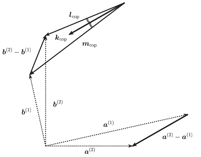
Note that each vector is given in the polar representation in and that bisects the angle between and . In addition to these relations, there is another constraint (3.28), which has a form
| (4.21) |
by (3.5c). Here we have selected the bulk solutions on both intervals with the minus sign case of (3.5c). Although it is possible to consider the other combination of the sign in (3.5c), the following analysis can be achieved similarly. Hence, we fix the matching condition as (4.21). By graphical analysis, we find the relations (4.19) and (4.20) have solutions with continuous parameters. When , both and , and and have the same directions so that the vector relations are shown as in Figure 1. When , those are shown as in Figure 2.

The moduli space dimensions, i.e., the number of continuous parameters minus the number of constraints, for the type- matching can be obtained by explicit counting of them. In this case, the parameters in the solution are the following 16:
| (4.22) |
and the constraints on these parameters are (4.19), (4.20) and (4.21), The first two constraints are the constraints on vectors in , so these are respectively two constraints in general. However, all of the vectors are given by polar representation, in which the origins of the angle ’s and can be freely chosen, thus we can always let one component in each constraint . Hence, the constraints (4.19) and (4.20) are the only relations for the norm of both sides, respectively. In fact, the second components of (4.19) and (4.20) are obtained from the first components of them by the shift of the angle and , and vice versa. Therefore, we conclude that the number of constraints are 3 for this case: the number of free parameter is . In addition to this, there should be a degree of freedom of global gauge rotation, which has 3 independent parameters for framed moduli space as in the case of instantons in . Therefore, the moduli space dimensions for is , which is the maximal number to calorons.
4.1.2 Type- matching conditions
Next, we consider the type- matching conditions, whose boundary data are given by (3.51). In this case, the matrix part of the matching conditions (3.2.1) can be recast to
| (4.23) | |||
| (4.24) |
where the vectors in the right-hand-side are, from (3.51b) – (3.51e),
In addition, from (3.5c) and (3.51a), we find
| (4.31) |
We now show that is necessary for the type- matching conditions, i.e., is not a moduli parameter. If we assume that , then it is found from (4.1.2) and (4.1.2) that and is orthogonal to by clockwise rotation. However, as can be seen in Figure 3, this is not allowed configuration due to the unfavorable orientation.

Hence, it is acceptable only for the type- matching. In this case, the matching conditions (4.23) and (4.24) reduce to and . They are fulfilled by and,
| (4.32a) | |||
| (4.32b) | |||
or
| (4.33a) | |||
| (4.33b) | |||
Having eliminated redundant parameters, we find that the moduli parameters for this configuration are
| (4.34) |
with constraints (4.32) or (4.33), and (4.31). Thus, the framed moduli space dimensions of the type- matching is . Note that the special case of the type- matching conditions is investigated in detail in [24].
4.1.3 Type-O matching conditions
The third type of matching conditions is the orthogonal type (3.2.2). For this case, we find the matching conditions can be regarded as vector relations in , along with two independent relations on ’s, in contrast to the type-P matching . That is, if we define
then the first and the third columns of (3.2.2) are equivalent to
| (4.49) | |||
| (4.50) |
where the three-vectors and are defined by (3.64c) and (3.64d), respectively. In (4.49) and (4.50), all the three components are independent each other, because they are not in the special form as in the type-P matching conditions. The rest of the matching conditions are,
| (4.51) | |||
| (4.52) |
Hence, we have 8 independent constraints.
We can observe that there actually exist solutions to this type of matching conditions. For example, if we take , then the matching conditions for and turn out to be
| (4.53a) | |||
| (4.53b) | |||
| (4.53c) | |||
| (4.53d) | |||
together with . It can be found that there exists a parameter region for and which enjoys (4.53) provided that .
In general, for the type-O matching conditions, the parameters in the solutions are the following 18,
| (4.54) |
subject to the 8 constraints (4.51), (4.52), (4.49) and (4.50). Therefore, the dimension of the framed moduli space for the type-O matching conditions are , where the comes from a global gauge transformation.
4.2 The (non-M, M) and (M, M) bulk data
In this subsection, we consider the cases that at least one of the bulk solution is the monopole type, namely, the (non-M, M) and (M, M) bulk solutions. Note that, for the (M, M) bulk data, we can always perform a “diagonalization” on one of the interval , say, by using a gauge transformation (2.13a). That is, we can fix the part of the bulk data on the interval to be
| (4.55a) | |||
| (4.55b) | |||
| (4.55c) | |||
for the (M, M) solutions.
4.2.1 Type- matching conditions
The type-P matching conditions of the matrix part (3.2.1) for the (non-M, M) bulk data are, by using (3.5), (3.3),
while for the (M, M) bulk data are
where is re-defined after the gauge transformation which diagonalize the bulk data on . From this consideration, we find that the (M, M) data are obtained by restricting in the (non-M, M) solutions. Hence, it is sufficient to consider the (non-M, M) solutions.
As in the previous subsection, we firstly consider the type- matching conditions. By using the 2-vectors (3.4), (4.1.1) and (4.18), we can recast (4.2.1) to,
| (4.72) | |||
| (4.73) |
where
| (4.74) |
Here, the “vectors” and are not in polar representations of vectors in , in contrast to the (non-M, non-M) solutions. As a consequence, there are 2 independent constraints in both (4.72) and (4.73). We find that the total number of constraints in the type- matching is 2+2+1=5, where 1 comes from (4.21), and that the parameters in the solution are the same as (4.22), except for for the (M, M) solution. Hence, the moduli space dimensions to this case are 16-5+3=14 for the (non-M, M) solution and 13 for (M, M) solution.
4.2.2 Type- matching conditions
Next, we consider the type- matching conditions, which are obtained by replacing (3.48) with (3.51), as for the (non-M, non-M) bulk data. The matching conditions are (4.31) along with
| (4.75) | |||
| (4.76) |
where the right-hand-sides are given by (4.1.2) and (4.1.2). In this case, the graphical situation is similar to Figure 3 so that it is necessary as in the (non-M, non-M) case. Hence, we find (4.75) and (4.76) are equivalent to
| (4.77a) | |||
| (4.77b) | |||
| (4.77c) | |||
| (4.77d) | |||
for the (non-M, M) case. These four constraints are independent each other as the type- matching conditions, so that there are totally constraints. The parameters in the solution to this matching conditions are the following ,
| (4.78) |
Accordingly, we find the dimensions for framed moduli space are .
As mentioned before, we can fix for the (M, M) case, which induces from (4.77). Thus, the moduli parameters are the following ,
| (4.79) |
The moduli space dimensions are for the (M, M) case, consequently.
4.2.3 Type-O matching conditions
Finally, we consider the matching conditions of the type-O. As in subsection 4.1.3, we can recast the matching conditions into the relations in . From the bulk data (3.3) and (3.5), and the matching conditions (3.2.2), we find
for the (non-M, M) solution, where and are defined by (3.64c) and (3.64d), respectively. The matching conditions for the (M, M) solution are obtained by restricting , as in the previous subsection.
4.3 Summary of this section
In this section, we have considered the framed moduli space dimensions for diverse types of matching conditions, which are summarized in the following table:
| Matching type | P | O | ||
|---|---|---|---|---|
| Bulk solutions | ||||
| (non-M, non-M) | 16 | 12 | 13 | |
| (non-M, M) | 14 | 11 | 13 | |
| (M, M) | 13 | 9 | 12 | |
We have found the calorons with -dimensional moduli space appear when the bulk solutions are of the type (non-M, non-M) and the matching conditions are of the type-.
5 The monopole and instanton limits
In this section, we consider the large scale limit, , and the large period limit, , of the caloron Nahm data obtained so far. Naively, they correspond to monopoles in and instantons in , respectively. Thus calorons are expected to interpolate between monopoles in and instantons in . However, as we will see in this section, things are somewhat complicated.
5.1 The monopole limit
It can easily be found that the separation between the center of two “2-monopoles” diverges at the large scale limit. In fact, from (3.2.1) and (3.66), we find that in the type- and the type-O matching at the limit of and/or . Also from (3.50), leads in the type- matching. Simultaneously, the parameters in the bulk Nahm data have to be
| (5.1) | |||
| (5.2) |
according to the matching conditions.
In these large scale limit, there remains only the bulk Nahm data on one of the intervals , say. Hence, if is the monopole type solution (3.3), then we find the BPS two-monopole configuration in this limit. On the other hand, if is the non-standard monopole type solution (3.5), we obtain the BPS two-monopole limit in its spatial rotated one. However, there should be another type of the large scale limit, the (2,1)-calorons, in general. To find the procedure to induce such kind of the large scale limits is under investigation.
5.2 The instanton limit
As mentioned above, it is expected that calorons turn out to be instantons on , in the large period limit . In this subsection, we will show that there are some restrictions on the caloron Nahm data which reproduces instanton limit. We have two approaches to obtain the instanton ADHM data from the caloron Nahm data with non-trivial holonomy. The first approach is that we take with the “monopole mass ratio”, , fixed during the process. In this approach, it is necessary that the bulk Nahm data of both intervals coincide, as we will see. The other approach is that we take via the calorons with trivial holonomy. Namely, if we firstly take the limit (or by the rotation map) to let one of the two-monopole be massless, then we obtain the Harrington-Shepard type calorons. It is known that those calorons have instanton limit without restriction. Hence, we only consider the first approach here.
Firstly, we consider the calorons of type-P matching conditions at the limit . The relations between each monopole mass and the period are given in terms of the monopole mass ratio as,
| (5.3) |
where is defined as
| (5.4) |
It is observed that the period and the scale parameters of calorons, and for type-, and for type-, are linked by the matching condition (3.28). By taking the limit, the left-hand-side of (3.28) turns out to be
| (5.5) |
while the right-hand-side is given by (3.48a) for the type- and (3.51a) for the type- matching conditions. This means that the scale parameters and/or must tend to be zero when . Accordingly, we find that all the components in the right-hand-side of (3.2.1) are zero when , from (3.48) for the type- or (3.51) for the type- matching conditions, respectively. Thus, we observe that (3.2.1) with turns out to be
| (5.6a) | |||
| (5.6b) | |||
or
| (5.7a) | |||
| (5.7b) | |||
according to the bulk Nahm data (3.3) or (3.5), and (3.4). Note that if then we find there is no solution for and in this limit. Hence, we conclude that all the parameters in the bulk Nahm data for both intervals have to coincide, i.e., , and at . In particular, is necessary for the case (5.7).
Consequently, from (3.28) and (5.5), the dependence of the scale parameters is
| (5.8a) | |||
| (5.8b) | |||
where the introduction of is for later convenience and (5.8b) appears only for the type-. Here, the parameters are subject to
| (5.9) |
for the type- matching case, and
| (5.10) |
for the type- matching case.
Now, we explicitly show the instanton ADHM data given by the large period limit of the calorons considered so far. Apparently, the interval turns out to be infinitesimal at , so that the bulk Nahm data are given by the value at . This means that only the solution in the interval is relevant. Hence, the instanton data obtained from the type- matching conditions with the non-standard monopole type bulk solution (3.5) are
while with the monopole type bulk solution (3.3) are
| (5.19) |
where and the condition (5.9) holds. For the latter case, we have performed the gauge transformation to be . Similarly, we find the instanton data from type- matching conditions are analogous to (5.2) and (5.19), but replaced the first rows with
| (5.20) |
along with (5.10).
Finally, we comment on the large period limit of type-O matching conditions. From (3.2.2) and (3.64), we find , which leads to a pure gauge configuration. Hence, there is no instanton limit in this case. If we need the instanton data from this type of matching, we have to take through the trivial holonomy calorons.
6 Conclusion
In this paper, we have constructed the analytic Nahm data of calorons of instanton charge . Although a part of analytic data has already been considered in [20, 22, 23, 24] along with numerical studies, this paper presents the Nahm data in its appropriate form to investigate the moduli space . The exact bulk data are given in (3.1) (3.3), (3.4) and (3.5). In particular, we have found that the Nahm data of (non-M, non-M) with type- matching conditions gives the case of maximal number of moduli parameters, 16, which is . In addition, the Nahm data of these forms are suitable for considering the large scale and the large period limit of the calorons.
It is expected that there exist higher charge () calorons with special symmetry, as symmetric monopoles. In order to search for such calorons, the non-standard monopole type solutions like (3.5) to the Nahm equation will play a significant role, as we have seen in the calorons. It will be suggested that the comprehensive study on the analytic solutions to Nahm equations provides further insight into the relationship between calorons, monopoles, and instantons.
Acknowledgement
The authors wish to thank Dr. Derek Harland for helpful comments. They are also grateful to Dr. Benoit Charbonneau for informing us about the references.
References
- [1] H. Garland, N.K. Murray, Comm. Math. Phys. 120 (1988) 335.
- [2] P. Norbury, Comm. Math. Phys. 212 (2000) 557.
- [3] B.J. Harrington, H.K. Shepard, Phys. Rev. D17 (1978) 2122; B.J. Harrington, H.K. Shepard, Phys. Rev. D18 (1978) 2990.
- [4] A. Chakrabarti, Phys. Rev. D35 (1987) 696.
- [5] M.F. Atiyah, V.G. Drinfeld, N.J. Hitchin, Yu.I. Manin, Phys. Lett. A65 (1978) 185.
- [6] W. Nahm, Self-Dual Monopoles and Calorons, in: Springer Lecture Notes in Phys., vol. 201, 1984, pp. 189-200.
- [7] T.M.W. Nye, arXiv:hep-th/0311215.
- [8] B. Charbonneau, J. Hurtubise, arXiv:0705.2412[math-DG]
- [9] D. J. Gross, R. D. Pisarski, L. G. Yaffe, Rev. Mod. Phys. 53, (1981) 43.
- [10] K. Lee, C. Lu, Phys. Rev. D58 (1998) 025011.
- [11] T.C. Kraan, P. van Baal, Phys. Lett. B428 (1998) 268; T.C. Kraan, P. van Baal, Nucl. Phys. B533 (1998) 627; T.C. Kraan, P. van Baal, Phys. Lett. B435 (1998) 389.
- [12] D. Diaknov, N. Gromov, Phys. Rev. D72 (2005) 025003.
- [13] N. Gromov, S. Slizovskiy, Phys. Rev. D73 (2006) 025022.
- [14] S. Slizovskiy, Phys. Rev. D76 (2007) 085019.
- [15] D. E. Diaconescu, Nucl. Phys. B503, (1997) 220.
- [16] K. Lee, P. Yi, Phys. Rev. D56 (1997) 3711; K. Lee, Phys. Lett. B426 (1998) 323.
- [17] A. Kapustin, S. Sethi, Adv. Theor. Math. Phys. 2 (1998) 571
- [18] E. Witten, JHEP 0906, 067 (2009)
- [19] S. A. Cherkis, arXiv:0902.4724 [hep-th]
- [20] D. Nógrádi, arXiv:hep-th/0511125.
- [21] G. Etesi, M. Jardim, Comm. Math. Phys. 280 (2008) 285.
- [22] F. Bruckmann, D. Nógádi, P. van Baal, Nucl. Phys. B666 (2003) 197.
- [23] F. Bruckmann, D. Nógádi, P. van Baal, B698 (2004) 233.
- [24] D. Harland, Journ. Math. Phys. 48 (2007) 082905
- [25] R.S. Ward, Phys. Lett. B582 (2004) 203.
- [26] N.J. Hitchin, Comm. Math. Phys. 89 (1983) 145.