An optical device for ultra-cold neutrons -
Investigation of systematic effects and applications
Abstract
We developed an optical device for ultra-cold neutrons and investigated the influence of a tilt of its guiding components. A measurement of the time-of-flight of the neutrons through the device by means of a dedicated chopper system was performed and a light-optical method for the alignment of the guiding components is demonstrated. A comparative analysis of former experiments with our results shows the potential of such a device to test the electrical neutrality of the free neutron on the level and to investigate the interaction of neutrons with gravity.
Keywords:
Neutron electric charge , Neutron optics , Ultra-cold neutronsPACS
03.75.Be , 28.20.Gd1 Introduction
Electric charge quantization (ECQ) and atom neutrality are well-established experimental observations. Their understanding is a long standing question of basic interest. ECQ implies that the charges of all known particles can be derived from integer multiples of one fundamental charge namely that of the electron. Early attempts to explain ECQ in the framework of quantum electrodynamics, like Dirac’s assumption of magnetic monopoles [1], still lack in experimental evidence.
In today’s framework of the Standard Model (SM), the quantization of charge is associated with the classical structure of the theory (i.e. gauge invariance) and the cancellation of quantum anomalies. As stated in [2, 3, 4], ECQ might not be a natural consequence of this model but can be effectuated with additional constraints to the SM Lagrangian by adding right-handed neutrino masses with Dirac and Majorana terms. The theoretical situation is ambiguous however, as the presence of these terms could also shift the electric charges of the known particles by an amount proportional to their baryon-lepton number [5]. As a consequence, so called ÔneutralÕ particles like the neutron could carry a small ’rest charge’.
In superstring models or grand unified groups, ECQ is a natural result of the theory [6, 7]. But also conventional extensions to the SM could lead to ECQ with the appearance of new fermions [3]. On the contrary, other hypotheses concern a new class of SU(2) U(1) models, where dequantization of the electric charge can occur by a nonzero photon mass [8] or by mini-charged Higgs bosons which couple to fermions [9]. In [10] it is suggested, that the charges of quarks and leptons, including neutrinos, and also of the proton and the neutron could have changed with the evolution of the Universe in time to a resulting present finite rest charge of the neutron or the neutrino. Assumptions beyond the conventional framework suggest topological shifts of the SM electric charges, where ordinary particles carry quantum hairs under massive higher spin fields (see [5] and references therein) resulting in charged atoms and neutrons.
We recall from [11] that a non-zero neutron charge would not be inconsistent with the conservation of the electric charge, the baryon and the lepton number. It would rather imply that conservation of the baryon number and conservation of the electric charge are not independent fundamental symmetries. Assuming charge conservation, a non zero value of would eliminate the possibility of neutron-antineutron oscillations [12], which is a candidate for a violation of the baryon number by .
Today’s accuracy on atom neutrality has reached a sensitivity of [13] and hence is comparable to direct limits on the neutron charge [14]. However, in [15] it is pointed out, that the charges of bound and free neutrons might not be identical. This would constrict results on the upper limit of the neutron charge obtained from indirect measurements on unionized atoms and molecules.
2 Direct measurements of
Experiments searching for an electric charge of the free neutron were carried out shortly after neutron beams were available from reactor sources. Shapiro and Estulin tried to deflect neutrons in a strong electric field [16] and reached a sensitivity of . A significant improvement of this approach was achieved by means of neutron optical elements with crystals or gratings in order to detect shifts of the beam profile or its angular deviation. Shull et al. [15] obtained a value for the ratio of the neutron over the proton charge, using a double crystal spectrometer, as .
3 Present experimental situation
The most precise direct limit on the free neutron charge was achieved 20 years ago with a setup described in [14] using a beam of cold neutrons at the Institut Laue-Langevin (ILL) in Grenoble / France. The result was:
| (1) |
About the same time, another experiment was performed with ultra-cold neutrons (UCN) at the VVR-M reactor in Gatchina / Russia [17]. The experiment had a discovery potential of . Due to a measuring time of only three days and a certain misalignment of the device, the final result was:
| (2) |
These direct measurements have in common that a beam deflection of a charged particle depends on the square of its traveling time in an electric field :
| (3) |
where is the charge and is the mass of the particle.
The measurement is carried out on the steep slope of the beam profile where the gradient is maximum. At this point the beam deflection is most sensitive to a difference in the count-rate with respect to a reversal of the electric field from to , and:
| (4) |
A neutron electric charge would cause a change in the count-rate according to:
| (5) |
If is determined with a statistical uncertainty (assuming ) in a measuring time , the sensitivity on (i.e. the discovery potential) is:
| (6) |
now is the mean square transit time of a neutron velocity spectrum through the experiment. In first approximation, the obtained beam profile has a Gaussian shape. At the steep point of the slope:
| (7) |
where is the width of the beam profile. Therefore:
| (8) |
We consider (8) a figure of merit and compare the experiments with cold neutrons [14] and with UCN [17] in tab. 1. Note that despite the high gain factors for and in the cold-neutron-experiment, the UCN experiment takes advantage of the much larger flight time of the ultra-cold neutrons in the region of the electric field. Nevertheless, the sensitivity of [17] is 16 times smaller compared to [14].
| Experiment | ||||
|---|---|---|---|---|
| [14], CN | ||||
| [17], UCN | ||||
| Gain factor | 23 | 6 |
The availability of highly intensive UCN sources (see [18] and references therein for a comprehensive overview) at different research centers such as PSI (Switzerland), ILL (France), LANL (USA), KEK (Japan), FRM II, or TRIGA Mainz (both Germany) will significantly improve the measurement sensitivity of many experiments and will also trigger new experimental approaches. Besides our attempt we mention as one example the GRANIT, a follow-up project based on an UCN spectrometer of ultra-high resolution, which provides accurate studies of/with the quantum states of neutrons in Earth’s gravity field [19]. A test of is also proposed in that paper.
4 Experimental setup
Our experiment was installed at the TES beamline of the UCN-facility PF2 [20] at ILL. UCN are guided via a 2.5 m long stainless steel tube of 70 mm diameter from the exit of the UCN turbine to the experiment. To protect the turbine vacuum and for safety reasons, a aluminum foil is permanently installed directly after the exit of the turbine.
Figure 1 shows a scheme of the experiment; the directions are indicated; is the direction of gravity. The vacuum is about during all measurements. Information on the used materials is given in the following section.
At the entrance of the experimental chamber the circular beam cross section is converted into a rectangular shape by means of a nickel guide (a) of inner dimensions and 34 cm length. After the rectangular guide, the UCN pass an entrance grating (b), which is shown in detail also in fig. 2. The grating has an overall dimension of . The slits are 0.4 mm or 0.7 mm wide and are separated by a distance of 1.5 mm. The lattice constant is therefore 1.9 mm or 2.2 mm. This entrance grating fragments the beam profile, and transmitted UCN are reflected between two horizontal neutron guide plates (c). The vertical distance between the plates is 50 mm, the dimensions of the plates are: Length 500 mm, width 100 mm, thickness 8 mm.
The upper plate lies on four adjustable nose-pieces sticking out of aluminum bars (d). The lower plate is supported at three positions; on two nose-pieces and on one linear actuator (e, see also fig. 6) which is movable in -direction.
UCN of too high divergence in -direction leave the device to the sides and are absorbed by borated rubber in the experimental chamber.
The device can be described as an optical camera for ultra-cold neutrons: A certain fraction of UCN reaches the end of the guide plates and encounter a mirror of cylindrical shape (f) in the horizontal -direction. The mirror has a curvature of 500 mm with dimensions in -direction. It reflects the UCN and focuses the image of the entrance grating back onto an exit grating (g). The latter is of same dimensions as the entrance grating. Together with a detector (h) mounted directly behind, it can be shifted along the -direction by a linear stage (i) in order to scan the reflected beam image. In the following, we refer to the detector together with the exit grating as the ’exit channel’.
The electrodes would be situated perpendicular to the guide plates generating an electric field in the -direction along the neutrons’ flight path. In the present setup we did not implement a HV system.
5 Materials and alignment
General remarks: We recall that the interaction of slow neutrons with matter can be described by a potential of the form:
| (9) |
where and are derived from parameters of the material surface at
which the neutrons interact via the strong force (see e.g. [21]).
In general, is called the ’wall potential’.
It defines a critical velocity below which a neutron
is reflected under any angle of incidence from the surface. The non-vanishing probability of absorption is described by the imaginary part
of (9).
As an example we cite the values for nickel: and [21].
Gratings: For the gratings, a material of high UCN absorption probability is required, which can also
be machined with high precision. We chose titanium of 1 mm thickness for the first. Ti is an effective UCN absorber
with a negative wall potential of and an absorption cross section
of 6.9 barn at [21].
The transmission probability for 1 mm Ti is for UCN of v=7 m/s.
The gratings were manufactured by CNC wire-erosion with a precision
of .
Guide plates: High specularity is required for the neutron guide plates, because diffusive reflection on the surface will lead to a misalignment of the UCN trajectories. We have chosen float-glass for the guides. Off-the-shelf, this material provides a high quality for surface roughness, typically on the order of . Note that the wavelength of UCN is on the order of some . In first order the probability for non-specular UCN reflection scales with [22]. Therefore float-glass is of first choice11 1 Note that high-quality UCN guides with an even lower surface roughness about 1 Å have been used in [23, 24].. Its wall potential () can be increased by coating of the reflecting surface with a non-conductive material22 2 Nickel for the coating as well as titanium for the gratings might not be suitable materials once the high voltage is implemented. like BeO (, used e.g. in [17]), diamond-like carbon (, [25]) or cubic boron nitride (, [26]).
Mirror: A material of high wall potential has to be used for the surface of the mirror, because UCN with their main velocity component have to be reflected. We chose N-BK 7 glass, which was coated with a layer of nickel. The surface finishing of the glass is 10 Å and the precision of the curvature radius is .
Detector: The detector is a lithium-doped glass scintillator (GS 10 see [27]) of dimension which is coupled via a transition light guide to a photomultiplier. It does not cover the whole area of the exit channel33 3 The detector was on loan from LPC Caen / France.. Therefore we placed the scintillator centered behind the exit grating with a shielding of borated rubber around it. With respect to its chemical composition, the scintillator has a wall potential comparable to float-glass. Therefore only UCN with velocities higher than 4.3 m/s can be detected.
Alignment: The adjustment of the entrance grating and the mirror with respect to the TES beamline was done with a laser. The guide plates were adjusted parallel to each other by a high-precision water-level. After closing the experimental chamber, a fine-tuning was performed by means of the linear actuator and with the observed neutron signal (see sec. 6).
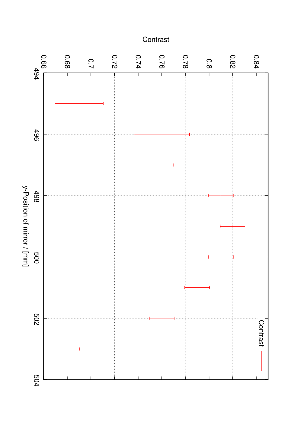
The mirror was placed about its focus point 500 mm behind the entrance grating. The optimum position was found with a light-optical method before closing the experimental chamber: We placed an array of LEDs before the rectangular guide and a photodiode at the position of the detector. By moving the exit channel with the linear stage, we observed a modulation of the light intensity. The average contrast of this curve is shown in fig. 3. The mirror was placed at the -position of the maximum contrast.
6 Modulation measurements
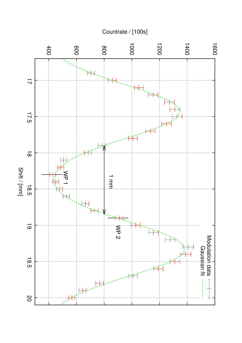
Figure 4 shows the UCN count-rate with the gratings of slit size 0.4 mm. Starting from the initial position at the exit channel is moved in steps of 0.2 mm away from the entrance grating and each position is measured for 100 s. We observe a modulation of the count-rate. The data are fitted by two Gaussian functions with the offset :
| (10) |
The fit parameters are summarized in tab. 2, .
| [1/100 s] | [mm] | [mm] | |
|---|---|---|---|
| 964 (60) | 0.375 (15) | 19.327 (7) | |
| 917 (60) | 0.369 (16) | 17.432 (8) |
The distance between the two peak positions, 1.89 (1) mm, corresponds to the lattice constant of the grating: (0.4+1.5) mm. From the minimum and the maximum count-rate (at and ) we derive the contrast . This maximum value was found after a fine-tuning of the lower guide plate (i.e. by a tilt of in -direction) by means of the linear actuator.
The count-rate at the steep slope of the modulation (we look at ) is , and the gradient at this point is . The average width of the obtained beam profile is .
7 Tilt measurements
We define two working points (WP) to investigate the influence of a tilt of the lower guide plate on the observed count-rate. The working points are indicated in fig. 1. We chose at the minimum and at the steep slope of the modulation44 4 These points do not fully coincide with the ones obtained from the fit: During the experiment, only a preliminary analysis of the modulation curve was carried out.. Figure 5 shows the observed count-rates at these working points when the lower guide plate is tilted in -direction about in steps of 0.025 mm. Around WP 1, the count-rate increases in both directions from the minimum. At WP 2 the count-rate rises or falls on a steep slope55 5 We mention that a similar behavior was observed when the lower plate was tilted at the points of the maximum of the modulation or at its steep slope of opposite gradient (i.e. at or at ). In the first case, we observed a decreasing of the count-rate in both directions from the maximum and in the second case, the steep slope is just of opposite orientation..
This can be understood in the following way: Undergoing a reflection at the tilted lower guide plate, a neutron gains velocity in the -direction as illustrated in fig. 6. The resulting -component depends on the tilt , on the -velocity and on the number of reflections of the neutron.
At WP 1 and without tilting, most of the neutrons hit the grating material of the exit channel and therefore a minimum in the modulation curve is observed. With a shift of the neutron trajectories caused by a tilt of the lower guide plate, the count-rate is increased in both tilting directions. In other words: A tilt of the guide plate is in some sense equal to a shift of the exit channel. In this way, also the data around WP 2 can be interpreted: Due to the tilt of the lower plate, the neutron trajectories are shifted towards the minimum or the maximum position adjacent to WP 2.
A simplified model is used to further understand the results: We assume that neutrons with velocity components undergo only one reflection on the lower plate after about half of their total flight time between the entrance and the exit grating. The lower plate is tilted by and the resulting tilt angle is (see fig. 6). For mono-energetic UCN, the induced shift of a neutron arriving at the exit channel is:
| (11) |
is the length of the guide plate (500 mm) and its width (100 mm). For non-monochromatic UCN, will be different for each neutron. We can expect that due to the resulting broadening of the beam profile the count-rate will not rise or fall to the maximum and minimum values adjacent to WP 2 (i.e. 14/s and 4/s) when the lower plate is tilted further. This is indeed observed for tilt values , where a saturation of the count-rates (about 10/s and 7/s) shows up (see fig. 5).
We further test our assumption ’tilt equals shift’ by putting numbers into the model: A tilt of around WP 1 (see fig. 5) increases the count-rate to . Approximately the same enhancement is observed when the exit channel is shifted by (see fig. 4). We take (from the ToF measurements described in sec. 8) and . Further we assume a quadratic velocity dependence for between zero and 4.3 m/s, the critical velocity of float-glass, resulting in a mean value of . With these values and from the left part of (11) we calculate . This is more or less in agreement with the expected value of 0.5 mm.
One could argue that under the assumption of more than one reflection on the lower guide plate occurs and that the resulting shift of a UCN due to the tilting should be larger. However, a UCN beam shows a forward peaking on transmission through guides depending on the specularity of reflection [21]. This angular distribution was not taken into account in our model, but it will lead to smaller values for . Therefore, the derived value has to be interpreted as an upper limit.
We focus again on the working point WP 2 and investigate the influence of a tilt upon the count-rate around this point. A linear fit to the data as indicated in fig. 5 () yields the gradient .
What is the meaning of this value? Apart from forces acting on the neutrons perpendicular to their flight direction (which we aim to detect with such a device), any change of the experimental environment e.g. by vibrations or electrostatic forces can also give rise to misaligned UCN trajectories, as the guide plates might be tilted by small amounts.This would lead to false effects.
In a measuring time , a change in the UCN count-rate due to a tilt has to be smaller than the statistical uncertainty on . This is mandatory to verify a shift of UCN trajectories which may arise from perpendicular forces. Therefore:
| (12) |
Assuming a measuring time of 100 s, and the gradient from above, it follows .
Equation (12) comprises a most important systematic effect. Note that , as in (7). Therefore the acceptable tilt over a measuring time will scale with .
So far we considered tilting as a systematic effect, which leads to misaligned UCN and therefore affects the count-rate. A tilt of the guide plates could occur for example if an electric field is reversed and the attached guide plates are slightly shifted in -direction due to the electrostatic forces between the electrodes. Note, that such a force is on the order of 0.2 N, assuming an electric field of and dimensions as given in [17]. In fact, the authors of that paper observed such tilting effects and backtracked them to electrostatic forces.
Tilting of the whole device however can also be used to calibrate the experiment and to derive a value for , independent of the time-of-flight measurements presented in the next section. We will come back to this important point in the appendix A.
8 Time-of-flight measurement
We now address to the time-of-flight (ToF) of the UCN through the device. A chopper system was built with a second entrance grating (see fig. 2), that can be moved periodically in -direction across the first one. To gain in statistics, the 0.7 mm gratings at the entrance, and no grating at the exit channel was installed.
In order to measure the opening function of the chopper, we placed an array of LEDs in front of, and a photodiode behind the chopper. The opening function is shown in fig. 7. The chopper is fully open for about 15 ms. Taken into account the slopes we derive an effective opening time of 18 (2) ms. The starting signal for the ToF is delivered from a frequency generator, which also drives the actuating coil via an amplifier. This signal (see fig. 7) starts the data acquisition 30 (2) ms before the chopper is fully open. The time-offset has to be considered in the analysis of the ToF data.
Figure 8 shows the raw ToF data (red) taken in one hour of measuring time. The duty cycle of the chopper is . First, the background is fitted in the indicated region with a constant . Second, and the time-offset are subtracted from the raw spectrum. The corrected data (green) are also shown in fig. 8. A Gaussian function is fitted to the corrected data, resulting in , the net area , the mean time-of-flight and the width . To obtain , we analyze the data in the region around as indicated in fig. 8:
| (13) |
where is the count-rate of the ToF bin .
A velocity spectrum is derived from the corrected data using the transformations: and , see e.g. [28]. For the mean flight length we take , which follows from (see sec. 6) and (assuming a quadratic velocity dependence between 3.2 m/s, the aluminum cut-off of the safety window, and 7 m/s, the nickel cut-off of the mirror). Note, that a detailed analysis would have to take into account the opening function of the chopper as well as a more realistic assumption on the velocity distribution. However, we are interested in a qualitative understanding of the data for which this basic approach is sufficient.
The obtained velocity spectrum (green) is shown in fig. 9. We state: a) The minimum detected velocity is about . This has two reasons: First, the aluminum safety window at the exit of the turbine only transmits neutrons with . Second, the minimum velocity of detectable neutrons is due to the wall potential of the scintillator. b) The maximum about corresponds to the critical velocity of the nickel coated mirror. c) There is a significant contribution from neutrons above the nickel cut-off.
For two reasons these neutrons behind the Ni cut-off show up in the spectrum: 1) At the TES beamline, also neutrons with velocities higher than 7 m/s are delivered from the UCN turbine. This is shown in fig. 9 (red). In this measurement the detector was placed at the position of the mirror. Neutrons with velocities up to 15 m/s, so called very-cold neutrons (VCN), contribute to the spectrum. 2) The reflectivity for a UCN of energy , impinging perpendicular on a surface with a wall potential is given by [21]:
| (14) |
The reflectivity curve of the nickel mirror surface is also shown in fig. 9. Note, that due to the non-step-wise character of , also UCN above the Ni cut-off can be reflected. Apart from losses of the back-reflected UCN and the different dimensions of the mirror and the detector surfaces, the obtained velocity spectrum at the exit channel is in principle the convolution of the reflectivity curve with the velocity spectrum at the position of the mirror.
| Parameters and dimensions | Measured values | |||||||||
| UCN flux | Flight | Slit | Detector | Contrast | Countrate | Gradient | Offset | |||
| path [m] | size [mm] | area / [cm2] | [1/s] | [1/s] | ||||||
| Our experiment | 1 | 0.4 | 9 | 0.53 | 9.7 | 16.5 | 0.022 | 7 | 3.6 | |
| [17] | 1.8 | 0.7 | 20 | 0.28 | 280 | 205 | 0.12 | 5 | ||
| Comparison I | 8 | 0.56 | 1.75 | 2.2 | 0.5 | 29 | 12.5 | 5.5 | 28 | |
| Comparison II | ||||||||||
9 Analysis
Contrast: The ratio of the contrast values of the two experiments is . To explain this difference we assume, that the contrast is mainly affected by the roughness of the guide plates: Roughness leads to diffusive reflection (see e.g. [29] for an overview and experimental results), to a misalignment of UCN trajectories and to a broadening of the obtained image. Let us consider further that the roughness of the plates in both experiments is about the same. We cannot really prove this assumption at the moment but we state that a diffusive reflection factor of 1.4 % as given in [17] is quite a realistic value for float-glass in UCN applications (see again [29]). How much a UCN is misaligned in -direction on its way through the device scales with the number of reflections on the surface and therefore with the flight path. The ratio between the flight paths of the two experiments, 0.56, corresponds to the ratio of the contrast values. In this view, roughness of the surface has to be considered as an important parameter.
The quantum mechanical broadening in -direction due to Heisenberg’s uncertainty principle is:
| (15) |
This value is about 0.15 mm in our setup (for the grating with ). Therefore quantum mechanical broadening is not negligible and a further decrease of the slit size will not consequently result in a higher contrast or a steeper gradient.
Count-rate: The ratio of the count-rates in the two experiments is 29. We have to take into account several factors to understand this value: The UCN flux at the former VVR-M reactor was about a factor 5 smaller than at the most intensive beamline of PF2 (which is called EDM):
| VVR-M | ||||
| PF2, EDM |
Further, at ILL, the UCN flux at TES is about a factor 40 smaller compared to EDM66 6 We determined this ratio by a comparison of UCN transmission measurements through a nickel foil at both beamlines. Independently, this ratio was found in ToF measurements by M. Daum et al. [30] at these two beamlines., hence about .
In first order, the observed count-rate rate is proportional to the solid angle covered by the mirror and the detector area over the flight path. A larger slit size will increase the count-rate77 7 Experimental proof of these two statements during our measurements: With a mirror of only half dimension in -direction (i.e. 5 cm), the detected count-rate also decreased by a factor of 2. The modulation was also measured with the gratings of slit size 0.7 mm (before: 0.4 mm). In this configuration we observed an increase in count-rate about a factor of 2..
From these arguments, the comparison factors I in tab. 3 with respect to flight path, slit size and detector area are derived. Together with an additional loss factor of 1.5, arising from the transition from the circular to the rectangular guide (), the expected loss factor for our experiment is about 26 (Comparison II in tab. 3). This is quite comparable to the observed ratio of the count-rates as stated above.
Gradient: With respect to (7), we would expect a ratio of the gradient values comparable to the ratio of the count-rates, as the width of the obtained image for both experiments is about the same (0.74 mm in our experiment, see tab. 2, and about 0.8 mm in the former setup [17]). Note however, that the value in the former experiment is the one used for the analysis. Apart from a few runs with higher gradients, this cited number is the average value over the full beam time, where was continuously monitored [31]. The determined ratio of 12.5 has to be interpreted therefore as a lower limit.
Time-of-Flight: There is a difference in the value of both experiments by a factor of 5.5. This arises from a larger flight length and a smaller mean UCN velocity in the former setup. We were limited to detect UCN only above the wall potential of the scintillation detector; 4.3 m/s. This could be overcome by using another detector material like with a wall potential close to zero in combination with a semiconductor (see [32, 33]). To overcome the velocity limitation arising from the safety window (in our case: aluminum with ), the experiment would have to be shifted up in height by about half a meter in order to slow down the UCN. We state that the sensitivity increases significantly, if the mean velocity is about 2–3 m/s.
Offset and background: The ratio of the offset values, 28, corresponds to the ratio of the count-rates of the two experiments. This is another evidence for our above made assumption, that the contrast is mainly affected by the roughness of the guide plates. In other words: A higher count-rate will lead to an increase of misaligned UCN, which contribute to in the modulation curve. Therefore this offset cannot be interpreted as a pure background but as an immanent characteristic of the device, which mainly depends on the surface quality of the guide plates. The background itself was measured independently (by placing absorbing materials between the guide plates) and was found to be negligible in our experiment.
10 Summary
We revisited the experiment of [17], a test of the electric charge of the neutron, at the beam position TES of PF2 at the ILL, and we reproduced the relevant parameters of the former setup in good agreement. We investigated the apparently most important systematic effect88 8 Other systematic effects are discussed in [14] and [34] in consideration of using cold neutron. The conclusions are conferrable to UCN. of a tilt of the guiding components. The acceptable limit for such a tilt would be on the -level for our setup and scales with .
We used a light-optical method to adjust the reflecting mirror to its optimum position. As an online-monitor for the alignment of the device, independent of the observed UCN count-rate, this method will be further developed.
A direct measurement of the mean transit time and between the entrance grating and the exit channel, i.e. in the relevant region along the situated electrodes, was demonstrated by means of a dedicated chopper system.
In view of a test of the electric charge of the neutron we state, that the expected gain in UCN density and flux at one of the new UCN sources like [35] is about a factor 100 compared to PF2–EDM at ILL. With an upgraded experiment following the approach of [17] and with control, monitoring and active compensation of the tilt effect, a sensitivity on on the level within a measuring time of a couple of weeks can be reached.
Appendix A Calibration by gravitational shift
If the whole device in fig. 1 (i.e. gratings, guides plates and attached electrodes, mirror and detector) is tilted by an angle with respect to the -axes, the neutron image is shifted by gravity along the direction of the electric field. This effect was demonstrated in [17] and allows an independent determination of the mean square transit time. Assuming monochromatic UCN, there is a relation between the tilt and the shift :
| (16) |
As a result, the count-rate will change according to:
| (17) |
The authors of [17] carried out such a calibration under the assumption of a non-monochromatic velocity distribution, with the geometrical parameters of their device and a diffusive reflection factor of 1.4% for the guide plates. From the obtained calibration curve and the leveling of their device they derived . This value was in good agreement with the result obtained from independent time-of-flight measurements99 9 In [17] a value of is reported. Note, that this is the mean square transit time of the UCN through the whole device obtained from velocity spectra which were measured between the entrance and at the exit of the device. A mean velocity 5 m/s was found. From this it follows a mean square transit time of about along the electrodes; ..
Appendix B Gravitational attraction
Following a remark of A. Franck [36], by placing massive bodies along the UCN flight path (i.e. at the position of the electrodes), the interaction of neutrons with gravity could be measured with a similar setup as described above. Note, that the acceleration of a neutron (assuming and ) would be about . It is easy to show, that gravity forces in the same direction as the electric field can be realized on the order of , hence two orders of magnitude larger and surely detectable. Considering (12) however, the necessity to install and even more to move massive bodies of some next to the setup appears to be challenging. But with the non-ebbing interest of neutrons’ interaction with gravity [19] one should keep an eye on every chance.
We thank A. Franck from the JINR Dubna / Russia for stimulating discussions. This project is supported by the Carl-Zeiss-Foundation and is part of the priority program 1491, ’Precision Experiments in Particle and Astrophysics with Cold and Ultracold Neutrons’ of the Deutsche Forschungsgemeinschaft.
References
- [1] A. M. Dirac. Quantised singularities in the electromagnetic field. Proc. R. Soc. London, 133(A):60–72, 1931.
- [2] R. Foot, H. Lew, and R. R. Volkas. Electric charge quantization. J. Phys., G(19):361, 1993.
- [3] R. Foot. Electric charge quantization without anomalies? Phys. Rev. D, 49(7):3617–3621, Apr 1994.
- [4] A. Yu. Ignatiev and G. C. Joshi. Neutrino electric charge and the possible anisotropy of the solar neutrino flux. Phys. Rev. D, 51(5):2411–2420, Mar 1995.
- [5] A. Arvanitaki, S. Dimopoulos, A. A. Geraci, J. Hogan, and M. Kasevich. How to test atom and neutron neutrality with atom interferometry. Physical Review Letters, 100(12):120407, 2008.
- [6] J. Schwarz M. Green and E. Witten. Superstring Theory. Cambridge University Press, Cambridge, 1986.
- [7] G. Ross. Grand Unified Theories. Addison-Wesley, 1985.
- [8] A. Yu. Ignatiev and G. C. Joshi. Possible electric charge nonconservation and dequantization in SU(2) U(1) models with hard symmetry breaking. Phys. Lett. B, 381:216–220, 1996.
- [9] E. Takasugi and M. Tanaka. Charge nonconservation and charges of neutrinos, neutron and atoms. Phys. Rev. D, 44(11):3706–3708, Dec 1991.
- [10] A. Yu. Ignatiev and G. C. Joshi. Can the electric charges of elementary particles change with time? Phys. Rev. D, 48(9):4481–4483, Nov 1993.
- [11] G. Feinberg and M. Goldhaber. Microscopic tests of symmetry principles. Proc. Natl. Acad. Sci. USA, 45:1301, 1959.
- [12] G. L. Glashow. Neutrino 79. Proc. of the Int. Conf. on Neutrions Weak Interaction and Cosmology, 1:518–522, 1979.
- [13] C. S. Unnikrishnan and G. T. Gillies. The electrical neutrality of atoms and of bulk matter. Metrologia, 41:125–135, 2004.
- [14] J. Baumann, R. Gähler, J. Kalus, and W. Mampe. Experimental limit for the charge of the free neutron. Phys. Rev. D, 37(11):3107–3112, Jun 1988.
- [15] C. G. Shull, K. W. Billman, and F. A. Wedgwood. Experimental limit for the neutron charge. Phys. Rev., 153(5):1415–1422, Jan 1967.
- [16] I. S. Shapiro and I. V. Estulin. Concerning the electric charge of the neutron. Zh. Eksp. Teor. Fiz., 30:579–580, 1956.
- [17] Borisov Yu., Borovikova N.V., Vasilev A.V., et al. On the feasibility of using ultracold neutrons to measure the electric charge of the neutron. Zh. Tekh. Fiz., 58:951–958, May 1988.
- [18] V. Nesvizhevsky, C. Plonka-Spehr, K. Protasov, K. Schreckenbach, T. Soldner, and O. Zimmer, editors. Proceedings of the international workshop on particle physics with slow neutrons. NIM A, 2009.
- [19] V.V. Nesvizhevsky and K.V. Protasov. Quantum states of neutrons in the Earth’s gravitational field: State of the art, applications, perspectives. Edited book on trends in quantum gravity research, Nova science publishers, D. C. Moore, 2006.
- [20] Institut Laue-Langevin. The ILL Yellow Book. Institut Laue-Langevin, Grenoble, 2009.
- [21] D. Richardson R. Golub and S.K. Lamoreaux. Ultra-Cold Neutrons. Oxford Press, 1991.
- [22] A. Steyerl, H. Nagel, F.X. Schreiber, et al. A new source of cold and ultracold neutrons. Phys.Let. A, 116:347, 1986.
- [23] C. Plonka, P. Geltenbort, T. Soldner, and H. Häse. Replika mirrors - nearly loss-free guides for ultracold neutrons - measurement technique and first preliminary results. NIM A, 578(2):450–452, 8 2007.
- [24] V.V. Nesvizhevsky, G. Pignol, K.V. Protasov, et al. Comparison of specularly reflecting mirrors for GRANIT. NIM, A(578):435–438, 2007.
- [25] F. Atchison, T. Brys, M. Daum, P. Fierlinger, P. Geltenbort, R. Henneck, S. Heule, M. Kasprzak, K. Kirch, A. Pichlmaier, C. Plonka, U. Straumann, and C. Wermelinger. First storage of ultracold neutrons using foils coated with diamond-like carbon. Physics Letters B, 625(1-2):19–25, 10 2005.
- [26] Yu. Sobolev, Th. Lauer, Yu. Borisov, et al. Cubic boron nitride: A new prospective material for ultracold neutron application. arXiv:0901.1336, 2009.
- [27] http://www.appscintech.com/.
- [28] I. Altarev, M. Daum, A. Frei, et al. Neutron velocity distribution from a superthermal solid 2H2 ultracold neutron source. Eur. Phys. J. A, 37:9–14, 2008.
- [29] S. Heule. Production, Characterization and Reflectivity Measurements of Diamond-like Carbon and other Ultracold Neutron Guide Materials. PhD thesis, University Zürich, 2008.
- [30] M. Daum. private communication, 2008.
- [31] P. Iaydjiev. private communication, 2009.
- [32] J. Jakubek, P. Schmidt-Wellenburg, P. Geltenbort, M. Platkevic, C. Plonka-Spehr, J. Solc, and T. Soldner. A coated pixel device TimePix with micron spatial resolution for UCN detection. NIM A, 600(3):651–656, 3 2009.
- [33] J. Jakubek, M. Platkevic, P. Schmidt-Wellenburg, P. Geltenbort, C. Plonka-Spehr, and M. Daum. Position-sensitive spectroscopy of ultra-cold neutrons with Timepix pixel detector. NIM A, 607(1):45–47, 8 2009.
- [34] R. Gähler, J. Kalus, and W. Mampe. Experimental limit for the charge of the free neutron. Phys. Rev. D, 25(11):2887–2894, Jun 1982.
- [35] http://ucn.web.psi.ch.
- [36] A. Frank. private communication, see also article in Phys. Atom. Nuclei, to be published Oct. 2009.