Structured Sparse Principal Component Analysis

Given a matrix $X\in\mathbb{R}^{n\times p}$ of $n$ rows corresponding to $n$ observations in $\mathbb{R}^{p}$, the dictionary learning problem is to find a matrix $V\in\mathbb{R}^{p\times r}$, called the dictionary, such that each observation can be well approximated by a linear combination of the $r$ columns $(V^{k})_{k\in\{1,\ldots,r\}}$ of $V$ called the dictionary elements. If $U\in\mathbb{R}^{n\times r}$ is the matrix of the linear combination coefficients or decomposition coefficients, the matrix product $UV^{\top}$ is called a decomposition of $X$.

Learning simultaneously the dictionary $V$ and the decomposition $U$ corresponds to a matrix factorization problem (see [5] and reference therein). As formulated in [14] or [5], it is natural, when learning a decomposition, to penalize or constrain some norms or quasi-norms of $U$ and $V$, say $\Omega_{u}$ and $\Omega_{v}$ respectively, to encode prior information—typically sparsity—about the decomposition of $X$. This can be written generally as

where the regularization parameter $\lambda\geq 0$ controls which extent the dictionary is regularized¹¹ 1 From [14], we know that our formulation is also equivalent to two unconstrained problems, with the penalizations $\frac{\lambda}{2}\sum_{k=1}^{r}[\Omega_{v}(V^{k})]^{2}\!+\![\Omega_{u}(U^{k})]^{2}$ or $\lambda\sum_{k=1}^{r}\Omega_{v}(V^{k})\Omega_{u}(U^{k})$. . If we assume that both regularizations $\Omega_{u}$ and $\Omega_{v}$ are convex, problem (1) is convex w.r.t. $U$ for $V$ fixed and vice versa. It is however not jointly convex in $(U,V)$.

The formulation of sparse PCA considered in [12] corresponds to a particular instance of this problem, where the dictionary elements are required to be sparse (without the orthogonality constraint $V^{\top}V=I$). This can be achieved by penalizing the columns of $V$ by a sparsity-inducing norm, e.g., the $\ell_{1}$ norm, $\Omega_{v}(V^{k})=\left\|V^{k}\right\|_{1}$. In the next section we consider a regularization $\Omega_{v}$ which controls not only the sparsity but also the structure of the supports of dictionary elements.

The work of [1] considered a norm which induces structured sparsity in the following sense: the solutions to a learning problem regularized by this norm have a sparse support which moreover belongs to a certain set of groups of variables. Interesting sets of possible supports include set of variables forming rectangles when arranged on a grid and more generally convex subsets²² 2 We use the term convex informally here. It can however be made precise with the notion of convex subgraphs ([15])..

The framework of [1] can be summarized as follows: if we denote by $\mathcal{G}$ a subset of the power set of $\{1,\dots,p\}$, such that $\bigcup_{G\in\mathcal{G}}G=\{1,\dots,p\}$, we define a norm $\Omega$ on a vector $y\in\mathbb{R}^{p}$ as

where $(d^{\scriptscriptstyle G})_{G\in\mathcal{G}}\in\mathbb{R}^{p\times|\mathcal{G}|}$ is a $|\mathcal{G}|$-tuple of $p$-dimensional vectors such that $d^{\scriptscriptstyle G}_{j}>0$ if $j\in G$ and $d^{\scriptscriptstyle G}_{j}=0$ otherwise. This norm $\Omega$ linearly combines the $\ell_{2}$ norms of possibly overlapping groups of variables, with variables in each group being weighted by $(d^{\scriptscriptstyle G})_{G\in\mathcal{G}}$. Note that a same variable $y_{j}$ belonging to two different groups $G_{1},G_{2}\in\mathcal{G}$ is allowed to be weighted differently in $G_{1}$ and $G_{2}$ (by respectively $d_{j}^{\scriptscriptstyle G_{1}}$ and $d_{j}^{\scriptscriptstyle G_{2}}$).

For specific choices of $\mathcal{G}$, $\Omega$ leads to standard sparsity-inducing norms. For example, when $\mathcal{G}$ is the set of all singletons, $\Omega$ is the usual $\ell_{1}$ norm (assuming that all the weights are equal to 1).

We focus on the case of a 2-dimensional grid where the set of groups $\mathcal{G}$ is the set of all horizontal and vertical half-spaces (see Fig. 1 taken from [1]). As proved in (1, Theorem 3.1), the $\ell_{1}/\ell_{2}$ norm $\Omega$ sets to zero some groups of variables $\left\|d^{\scriptscriptstyle G}\circ y\right\|_{2}$, i.e., some entire horizontal and vertical half-spaces of the grid, and therefore induces rectangular nonzero patterns. Note that a broader set of convex patterns can be obtained by adding in $\mathcal{G}$ half-planes with other orientations. In practice, we use planes with angles which are multiples of $\frac{\pi}{4}$.

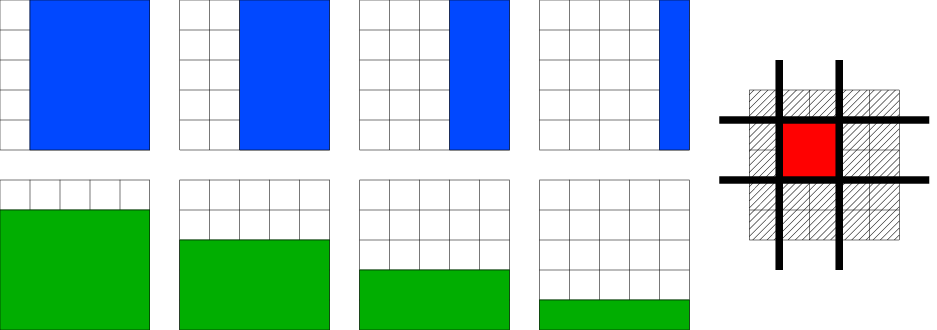
Among sparsity inducing regularizations, $\ell_{1}$ is often privileged since it is convex. However, so-called concave penalizations, such as penalization by an $\ell_{\alpha}$ quasi-norm, which are closer to $\ell_{0}$ and penalize more aggressively small coefficients can be preferred, especially in a context where the unregularized problem, here dictionary learning is itself non convex. In light of recent work showing the advantages of addressing sparse regression problems through concave penalization (e.g., see [16]), we therefore generalize $\Omega$ to a family of non-convex regularizers as follows: for $\alpha\in(0,1)$, we define the quasi-norm $\Omega^{\alpha}$ for all vectors $y\in\mathbb{R}^{p}$ as

where we denote by $(\left\|d^{\scriptscriptstyle G}\circ y\right\|_{2})_{G\in\mathcal{G}}\in\mathbb{R}^{1\times|\mathcal{G}|}$ the $|\mathcal{G}|$-tuple composed of the different blocks $\left\|d^{\scriptscriptstyle G}\circ y\right\|_{2}$. We thus replace the (convex) $\ell_{1}/\ell_{2}$ norm $\Omega$ by the (neither convex, nor concave) $\ell_{\alpha}/\ell_{2}$ quasi-norm $\Omega^{\alpha}$. Note that this modification impacts the sparsity induced at the level of groups, since we have replaced the convex $\ell_{1}$ norm by the concave $\ell_{\alpha}$ quasi-norm.

We are now considering Eq. (1) where we take $\Omega_{v}$ to be $\Omega^{\alpha}$, that is,

Although the minimization problem Eq. (2) is still convex in $U$ for $V$ fixed, the converse is not true anymore because of $\Omega^{\alpha}$. Indeed, the formulation in $V$ is non-differentiable and non-convex. To address this problem, we use the variational equality based on the following lemma that is related³³ 3 Note that we depart form [17, 18] who consider a quadratic upperbound on the squared norm. We prefer to remain in the standard dictionary learning framework where the penalization is not squared. to ideas from [17, 18]:

To reformulate problem $(2)$, let us consider the $|\mathcal{G}|$-tuple $(\eta^{\scriptscriptstyle G})_{G\in\mathcal{G}}\in\mathbb{R}^{r\times|\mathcal{G}|}$ of $r$-dimensional vectors $\eta^{\scriptscriptstyle G}$ that satisfy for all $k\in\{1,\dots,r\}$ and $G\in\mathcal{G}$, $\eta^{\scriptscriptstyle G}_{k}\geq 0$. It follows from Lemma (3.1) that

If we introduce the matrix $\zeta\in\mathbb{R}^{p\times r}$ defined by⁴⁴ 4 For the sake of clarity, we do not specify the dependence of $\zeta$ on $(\eta^{\scriptscriptstyle G})_{G\in\mathcal{G}}$. $\zeta_{jk}\!\!=\!\!\big\{\sum_{G\in\mathcal{G},\ G\ni j}(d^{\scriptscriptstyle G}_{j})^{2}(\eta^{\scriptscriptstyle G}_{k})^{-1}\big\}^{-1}$, we then obtain

This leads to the following formulation

which is equivalent to Eq. (2) and convex with respect to $V$.

So far, the regularization quasi-norm $\Omega^{\alpha}$ has been used to induce a structure inside each dictionary element taken separately. Nonetheless, some applications may also benefit from a control of the structure across dictionary elements. For instance it can be desirable to impose the constraint that $r$ dictionary elements share only a few different nonzero patterns. In the context of face recognition, this could be relevant to model the variability of faces as the combined variability of several parts, with each part having a small support (such as eyes), and having its variance itself explained by several dictionary elements (corresponding for example to the color of the eyes).

To this end, we consider $\mathcal{M}$, a partition of $\{1,\dots,r\}$. Imposing that two dictionary elements $V^{k}$ and $V^{k^{\prime}}$ share the same sparsity pattern is equivalent to imposing that $V^{k}_{i}$ and $V^{k^{\prime}}_{i}$ are simultaneously zero or non-zero. Following the approach used for joint feature selection ([19]) where the $\ell_{1}$ norm is composed with an $\ell_{2}$ norm, we compose the norm $\Omega^{\alpha}$ with the $\ell_{2}$ norm $V^{M}_{i}=\|(V^{k}_{i})_{k\in M}\|_{2}$, of all $i^{\text{th}}$ entries of each dictionary element of a class $M$ of the partition, leading to the regularization:

In fact, not surprisingly given that similar results hold for the group Lasso [17], it can be shown that the above extension is equivalent to the variational formulation

with class specific variables $\eta_{M}$, $\zeta^{M}$, $M\!\in\!\mathcal{M}$, defined by analogy with $\eta_{k}$ and $\zeta^{k}$, $k\!\in\!\{1,\dots,r\}$.

The main optimization procedure described in Algorithm 1 is based on a cyclic optimization over the three variables involved, namely $(\eta^{\scriptscriptstyle G})_{G\in\mathcal{G}}$, $U$ and $V$. We use Lemma (3.1) to solve Eq. (2) by a sequence of problems that are convex in $U$ for fixed $V$ (and conversely, convex in $V$ for fixed $U$). For this sequence of problems, we then present efficient optimization procedures based on block coordinate descent (BCD) (20, Section 2.7). We describe these in detail in Algorithm 1. Note that we depart from the approach of [1] who use an active set algorithm. Their approach does not indeed allow warm restarts, which is crucial in our alternating optimization scheme.

We first apply SSPCA on the cropped AR Face Database [21] that consists of 2600 face images, corresponding to 100 individuals (50 women and 50 men). For each subject, there are 14 non-occluded poses and 12 occluded ones (the occlusions are due to sunglasses and scarfs). We reduce the resolution of the images from 165x120 to 38x27 for computational reasons.

Fig. 2 shows examples of learned dictionaries (for $r=36$ elements), for NMF, SSPCA and SSPCA with shared structure. While NMF finds sparse but spatially unconstrained patterns, SSPCA select sparse convex areas that correspond to a more natural segment of faces. For instance, meaningful parts such as the mouth and the eyes are recovered by the dictionary.

We now compare SSPCA, SPCA (as in [12]), PCA and NMF on a face recognition problem. We first split the data into 2 parts, the occluded faces and non-occluded ones. For different sizes of the dictionary, we apply each of the aforementioned dimensionality reduction techniques to the non-occluded faces. Keeping the learned dictionary $V$, we decompose both non-occluded and occluded faces on $V$. We then classify the occluded faces with a k-nearest-neighbors classifier (k-NN), based on the obtained low-dimensional representations. Given the size of the dictionary, we choose the number of nearest neighbor(s) and the amount of regularization $\lambda$ by 5-fold cross-validation⁵⁵ 5 In the 5-fold cross-validation, the number of nearest neighbor(s) is searched in $\{1,3,5\}$ while $\log_{2}(\lambda)$ is in $\{4,6,8,\dots,18\}$. For the dictionary, we consider the sizes $r\in\{10,20,30,40,50,60,70\}$..

The formulations of NMF, SPCA and SSPCA are non-convex and as a consequence, the local minima reached by those methods are sensitive to the initialization. Thus, after having selected the parameters by cross-validation, we run each algorithm 20 times with different initializations on the non-occluded faces, divided into a training (900 instances) and validation set (500 instances) and take the model with the best classification score. We summarize the results in Fig. 3. We denote by shared-SSPCA (resp. shared-SPCA) the models where we impose, on top of the structure of $\Omega^{\alpha}$, to have only 10 different nonzero patterns among the learned dictionaries (see Section 3.2).

As a baseline, we also plot the classification score that we obtain when we directly apply k-NN on the raw data, without preprocessing. Because of its local dictionary, SSPCA proves to be more robust to occlusions and therefore outperforms the other methods on this classification task. On the other hand, SPCA, that yields sparsity without a structure prior, performs poorly. Sharing structure across the dictionary elements (see Section 3.2) seems to help SPCA for which no structure information is otherwise available.

The goal of our paper is not to compete with state-of-the-art techniques of face recognition, but to demonstrate the improvement obtained between $\ell_{1}$ and more structured norms. We could still improve upon our results using non-linear classification (e.g., with a SVM) or by refining our features (e.g., with a Laplacian filter).

Understanding the dynamics of protein complexes is important since conformational changes of the complex are responsible for modification of the biological function of the proteins in the complex. For the EF-CAM complex we consider, it is of particular interest to study the interaction between EF (adenyl cyclase of Bacillus anthracis) and CAM (calmodulin) to find new ways to block the action of anthrax [22].

In our experiment, we consider 12000 successive positions of the 619 residues of the EF-CAM complex, each residue being represented by its position in $\mathbb{R}^{3}$ (i.e., a total of 1857 variables). We look for dictionary elements that explain the dynamics of the complex, with the constraint that these dictionary elements have to be small convex regions in space. Indeed, the complex is comprised of several functional domains (see Fig. 4) whose spatial structure has to be preserved by our decomposition.

We use the norm $\Omega^{\alpha}$ (and $\mathcal{G}$) to take into account the spatial configuration. Thus, we naturally extend the groups designed for a 2-dimensional grid (see Fig. 1) to a 3-dimensional setting. Since one residue corresponds to 3 variables, we could either (1) aggregate these variables into a single one and consider a 619-dimensional problem, or (2) we could use Section 3.2 to force, for each residue, the decompositions of all three coordinates to share the same support, i.e., in a 1857-dimensional problem. This second method has given us more satisfactory results.

We only present results on a small dictionary (see Fig. 4 with $r=3$). As a heuristic to pick $\lambda$, we maximize $|\bigcup_{k=1}^{r}\!\mathrm{supp}\!\left(V^{k}\right)|^{2}/(p\sum_{k=1}^{r}\!|\mathrm{supp}\!\left(V^{k}\right)|)$ to select dictionary elements that cover pretty well the complex, without too many overlapping areas.

We retrieve groups of residues that match known energetically stable substructures of the complex [22] . In particular, we recover the two tails of the complex and the interface between EF and CAM where the two proteins bind. Finally, we also run our method on the same EF-CAM complex perturbed by (2 and 4) calcium elements. Interestingly, we observe stable decompositions, which is in agreement with the analysis of [22].

References

- [1] R. Jenatton, J-Y. Audibert, and F. Bach. Structured variable selection with sparsity-inducing norms. Technical report, 2009. preprint arXiv:0904.3523v1.
- [2] D. D. Lee and H. S. Seung. Learning the parts of objects by non-negative matrix factorization. Nature, 401:788–791, 1999.
- [3] I. T. Jolliffe, N. T. Trendafilov, and M. Uddin. A modified principal component technique based on the LASSO. Journal of Computational and Graphical Statistics, 12(3):531–547, 2003.
- [4] H. Zou, T. Hastie, and R. Tibshirani. Sparse principal component analysis. Journal of Computational and Graphical Statistics, 15(2):265–286, 2006.
- [5] D. M. Witten, R. Tibshirani, and T. Hastie. A penalized matrix decomposition, with applications to sparse principal components and canonical correlation analysis. Biostatistics (Oxford, England), April 2009.
- [6] L. Jacob, G. Obozinski, and J. P. Vert. Group Lasso with overlap and graph Lasso. In Proceedings of the 26th International Conference on Machine Learning, 2009.
- [7] J. Huang, T. Zhang, and D. Metaxas. Learning with structured sparsity. In Proceedings of the 26th International Conference on Machine Learning, 2009.
- [8] A. d’Aspremont, F. Bach, and L. El Ghaoui. Optimal solutions for sparse principal component analysis. Journal of Machine Learning Research, 9:1269–1294, 2008.
- [9] B. Moghaddam, Y. Weiss, and S. Avidan. Spectral bounds for sparse PCA: Exact and greedy algorithms. Advances in Neural Information Processing Systems, 18:915, 2006.
- [10] Lester Mackey. Deflation methods for sparse pca. In D. Koller, D. Schuurmans, Y. Bengio, and L. Bottou, editors, Advances in Neural Information Processing Systems 21, pages 1017–1024. 2009.
- [11] J. Mairal, F. Bach, J. Ponce, and G. Sapiro. Online dictionary learning for sparse coding. In Proceedings of the 26th International Conference on Machine Learning, 2009.
- [12] H. Lee, A. Battle, R. Raina, and A. Y. Ng. Efficient sparse coding algorithms. In Advances in Neural Information Processing Systems, pages 801–808, 2007.
- [13] A.P. Singh and G.J. Gordon. A Unified View of Matrix Factorization Models. In Proceedings of the European conference on Machine Learning and Knowledge Discovery in Databases-Part II, pages 358–373. Springer, 2008.
- [14] F. Bach, J. Mairal, and J. Ponce. Convex sparse matrix factorizations. Technical report, 2008. preprint arXiv:0812.1869.
- [15] F.R.K. Chung. Spectral graph theory. American Mathematical Society, 1997.
- [16] T. Zhang. Multi-stage convex relaxation for learning with sparse regularization. In Advances in Neural Information Processing Systems, pages 1929–1936, 2008.
- [17] F. Bach. Consistency of the group Lasso and multiple kernel learning. Journal of Machine Learning Research, 9:1179–1225, 2008.
- [18] C. A. Micchelli and M. Pontil. Learning the kernel function via regularization. Journal of Machine Learning Research, 6(2):1099, 2006.
- [19] G. Obozinski, B. Taskar, and M. Jordan. Joint Covariate Selection and Joint Subspace Selection for Multiple Classification Problems. Statistics and Computing, 2009.
- [20] D. P. Bertsekas. Nonlinear programming. Athena scientific, 1995.
- [21] A. M. Martinez and A. C. Kak. PCA versus LDA. IEEE Transactions on Pattern Analysis and Machine Intelligence, 23(2):228–233, 2001.
- [22] E. Laine, A. Blondel, and T. E. Malliavin. Dynamics and energetics: A consensus analysis of the impact of calcium on ef-cam protein complex. Biophysical Journal, 96(4):1249–1263, 2009.