Towards a Holographic Model of Color-Flavor Locking Phase

Preprint: MAD-TH-09-07
NSF-KITP-09-172
RIKEN-TH-166

Heng-Yu Chen Affiliation: Department of Physics, University of Wisconsin, Madison, WI 53706, USA^†Theoretical Physics Laboratory, RIKEN, Saitama 351-0198, Japan^§Kavli Institute for Theoretical Physics, University of California,Santa Barbara CA 93106-9530, USA Affiliation: E-mail: Email: hchen46@wisc.edu Koji Hashimoto Affiliation: E-mail: Email: koji@riken.jp Shunji Matsuura Affiliation: E-mail: Email: matsuura@kitp.ucsb.edu

Abstract:

We demonstrate a holographic realization of color-flavor locking phase, using ${\cal N}=4$ $SU(N_{c})$ SYM coupled to ${\cal N}=2$ $N_{f}$ fundamental hypermultiplets as an example. The gravity dual consists of $N_{c}$ D3-branes and $N_{f}$ D7-branes with world volume gauge field representing the baryon density. Treating a small number $\tilde{N}_{c}\subset N_{c}$ of D3-branes as Yang-Mills instantons on the D7-branes, we consider possible potential(s) on their moduli space or equivalently the Higgs branch. We show that a non-trivial potential can be generated by including the backreaction of the baryonic density on the D7-branes, this dynamically drives the instantons (= D3-branes) into dissolution. We interpret this as a color-flavor locking since the size of the instanton is the squark vev, and study the symmetry breaking patterns. Extending to finite temperature setup, we demonstrate that color-flavor locking persists, and the thermal effect provides additional structures in the phase diagram.

1 Introduction and Summary

In QCD phase diagram, the color-flavor locking (CFL) phase, or more generically, the color superconducting phase, is expected to be present in a region with large chemical potential $\mu$ for baryon number. Perturbative analytic study of this phase (see Ref. [1] for reviews) has mainly been done for very large $\mu$ such that the QCD coupling is weak. However, the issue on possible phase transitions from the hadronic phase at finite $\mu$ has not been addressed, as the system becomes strongly coupled. So far, neither direct experimental search, nor the lattice QCD simulation with “sign problem” have reached such region in the phase space.

Holographic techniques from gauge/string duality [2, 3] may offer new insights to such issue, as they enable us to probe the strongly coupled region(s) in the phase diagram for QCD-like theories. Although the duality strictly works for large number of colors $N_{c}\gg 1$ , the holographic techniques applied to QCD-like theories (so-called “Holographic QCD”) have been rather successful in reproducing qualitative and semi-quantitative features of low energy QCD dynamics. In this paper, among other things, we shall show that a color-flavor locking occurs for a toy QCD-like theory at zero temperature, when the baryon chemical potential $\mu$ exceeds its critical value.¹¹ 1 Disclaimer: Note that our theory is not QCD but rather a supersymmetric generalization of it, and we shall only treat the squark condensation for the CFL. For a field-theoretical treatment of the squark condensation, see for example Ref. [7].

Problems of CFL in Holographic QCD

Before entering the details on how to realize CFL phase in our model, let us summarize here the possible difficulties in obtaining it in holographic QCD.

•

In gauge/string duality, to treat $N_{f}$ flavor branes as probes, we typically need to take $N_{c}\gg N_{f}$ , while the CFL refers to a locking of the $SU(3)$ flavor and the $SU(3)$ color symmetries, i.e. $N_{c}=N_{f}$ .
•

In gauge/string duality, usually only gauge-invariant quantities are considered, while in the CFL phase the order parameter is a gauge variant di-quark condensate.

The first problem is strictly technical, as when $N_{f}\sim N_{c}$ , the backreaction of the flavor branes cannot be ignored, and renders it difficult to analyze in supergravity.²² 2 There are examples in which fully backreacted geometry is obtained (see for example Ref. [6]), and it would be interesting to generalize our results to those examples. Our approach used in this paper is to first separate some finite number of color branes $\tilde{N}_{c}$ (i.e. $\tilde{N}_{c}\ll N_{c}$ ), and investigate the locking of $SU(\tilde{N}_{c})$ color symmetry with the flavor symmetry. Though this procedure of separation is artificial, our result may suggest a piece of the whole picture. Another concern for the first problem is that in the strict $N_{c}\to\infty$ limit, the theory does not reveal the CFL phase [8]. We don’t consider this concern, since we will not perform a comparison with the chiral density wave (which is supposed to be favored at the strict $N_{c}\to\infty$ limit) in our toy model, and also because a large but finite value of $N_{c}$ may give the CFL phase even for the real QCD [9].

As for the second problem above, it is familiar to us that gauge-invariant correlators of QCD-like theories can be computed in their gravity duals, but in fact there are some gauge-covariant quantities which one can also compute in the gauge/string duality.³³ 3 Examples of that kind include computations explicitly uses string worldsheets in the dual gravity backgrounds; gluon scattering amplitudes, drag forces, quark-antiquark forces, heavy meson spectroscopy and Regge trajectory. In this paper, we use holographic techniques for Coulomb phase of supersymmetric Yang-Mills (SYM) theories [10, 11], where a part of the gauge symmetry decouples from the rest. When the rank of this decoupled gauge subgroup is small, we may treat them in the same way as the probe flavor branes, and their gauge symmetry is manifest in the dual gravity description. We shall describe this in detail later.

Supersymmetric QCD, the Holographic Dual and Phase Diagram

The toy model we shall focus on is ${\cal N}=4$ SYM coupled to ${\cal N}=2$ fundamental matter hyper multiplets. The holographic dual of this theory was proposed by Karch and Katz [12], as a minimal deformation of the ${\cal N}=4$ SYM to include quarks. The quark superfields are introduced as the lowest excitation on a string connecting $N_{c}$ D3-(color-)branes and $N_{f}$ D7-(flavor-)branes. For $N_{c}\gg N_{f}$ , D3-branes can be replaced by $AdS_{5}\times S^{5}$ geometry, and the flavor dynamics of the strongly coupled large $N_{c}$ SQCD can be analyzed by the probe flavor D7-branes in that geometry. The quark mass $m$ quark is proportional to the distance between the D3-branes and the D7-branes.

For zero temperature $T=0$ and $\mu=0$ , quarks and gluons are deconfined while quarks can form deeply bound mesons. The phase structure of this theory has been analysed by the holographic duality [13, 14, 19, 20, 21] and at the leading large $N_{c}$ expansion, it is known that there are two phases in the $(\mu,T)$ diagram: the meson phase and the melted meson phase (see Fig. 1).

Refer to caption — Figure 1: The structure of the phase diagram of the ${\cal N}=2$ SQCD. (Scales in this figure is not accurate. See [13, 14, 19, 20, 21] for details.)

In both phases, gluons are deconfined. In the meson phase, quarks are bound to form mesons with their discrete spectrum,⁴⁴ 4 The meson spectrum at zero baryon density is studied in Refs. [22, 23]. while in the melted meson phase, the meson spectrum is continuous, and there appears nonzero baryon number density. These two phases are characterized by the shape of the probe $N_{f}$ D7-branes [24, 29, 25, 26, 27, 28]. For the finite temperature, the background geometry is an AdS black hole. The meson phase corresponds to the D7-branes away from the horizon, which is called “Minkowski embedding”. On the other hand, in the melted meson phase, the D7-branes touch the horizon (see Fig. 2), and is called “black hole embedding”.

Since the local gauge symmetry $U(N_{f})$ on the D7-brane is identified as the global $U(N_{f})_{\rm V}$ symmetry of the SQCD via the gauge/string duality, the chemical potential $\mu$ is identified as the value of the temporal component of the overall $U(1)$ gauge field on the coincident D7-branes. In the meson phase, this gauge field is just a constant $\mu$ , while in the melted meson phase, there appears electric flux on the D7-branes: this configuration has a lower free energy which the holographic dual can compute, and thus favored. The phase transition is first order, and the critical chemical potential for $T=0$ is $\mu_{\rm cr}=m$ . In the melted meson phase, the shape of the D7-branes is a spike whose tip is inside the horizon. Electrically charged spikes on D-branes are identified as fundamental strings, so the existence of the electric flux means that the quark number density is nonzero. These are briefly reviewed in Sec. 2.1.

Dynamically Driven CFL

Let us explain how the CFL phase of this theory can be realized in its gravity dual. First of all, note that our theory is ${\cal N}=2$ SQCD which includes squarks carrying the baryon (quark) number. So, once the chemical potential becomes large enough, we expect squark condensation, instead of di-quark condensation. We shall see this squark condensation in this paper: this is certainly a CFL, but also a Higgs phase.

As suggested before, we separate $\tilde{N}_{c}$ D3-branes among $N_{c}$ and treat them as probes, $\tilde{N}_{c}\ll N_{c}$ . The relevant quark/squarks are strings connecting the $\tilde{N}_{c}$ D3-branes and the $N_{f}$ D7-branes. Condensation of strings connecting D $p$ -branes and D $(p+4)$ -branes is well-known [30]: the D $p$ -branes are dissolved into the D $(p+4)$ -branes, and the D $p$ -branes can be seen as finite size instantons on the D $(p+4)$ -branes. Therefore, the CFL Higgs phase of the SQCD is equivalent, via the gauge/string duality, to the situation where the size of the instantons on the probe D7-branes is driven to become larger. We will show in this paper that this is indeed the case, by computing the potential of the instanton size modulus on the D7-brane $U(N_{f})$ gauge theory, in the melted meson phase. D3-branes are moved onto the D7-branes and dissolve on the D7-branes dynamically.

This Higgs phase for $T=0$ was described in Refs. [31, 32, 33] (see also Ref. [34]), and the potential for the instanton size modulus was considered in the absence of baryon density. At $T=0$ , the resultant potential vanishes (we review it in Sec. 2.2 and 2.3), thus there is no CFL. Our new point is that including a backreaction from the D7-brane electric flux (Sec. 3), this generates a nontrivial potential for the intanton size modulus (Sec. 4). The new potential has a run-away behavior (see Fig. 5), causing the instantons to expand, hence the CFL Higgs phase is prefered. This new potential exists only in the melted meson phase, so, for $T=0$ , above the critical baryon chemical potential, the CFL Higgs phase appears — this is what we show using the gauge/string duality for the SQCD.

The way this new potential emerges is quite intriguing. This is essentially a Chern-Simons (CS) term on the D7-branes, $\int{\rm tr}\;F\wedge F\wedge F\wedge C_{2}$ . The backreaction of the electric flux on the D7-branes generate a nonzero constant Ramond-Ramond (RR) 3-form flux $F_{3}=dC_{2}$ (3.1).⁵⁵ 5 The importance of this coupling between the NSNS 2-form and the $F_{3}$ for the baryons was found in Ref. [5]. Substituting this to the CS term, we obtain $\int{\rm tr}\;A\wedge F\wedge F$ , thus the electric potential $A_{t}$ on the D7-brane interacts with the instanton density ${\rm tr}F\wedge F$ , which gives a nontrivial potential (4.9).⁶⁶ 6 A similar CS mechanism was used for treating baryons [41, 42] in Sakai-Sugimoto holographic model [43], but used in a rather different way: the CS term was to stabilize the size of a single baryon in the model. This generation of $F_{3}$ can also be thought of being sourced by baryon vertices, which are nothing but D5-branes wrapping $S^{5}$ [4] (see also Ref. [5]). If one smears them, they provide a constant magnetic flux $F_{3}$ along $x^{1}$ - $x^{2}$ - $x^{3}$ directions (Sec. 3.1). So, our work is an example of backreacting baryon vertices.

We also analyze the thermalized case with $T\neq 0$ (Sec. 5). Ref. [35] showed that, for the finite temperature, a nontrivial potential (5.30) for the size modulus of the instanton on the D7-branes is generated, before including the baryon density. This potential is minimized at a finite value of the instanton size. Therefore a Higgs CFL phase is prefered. Introducing baryonic density, we analyze the backreaction and our new CS-type potential (5.32) adds up on it. This addition does not change the result that the instanton size is nonzero, so we still have the Higgs CFL phase.

If we naively adds up the two potentials (the thermal potential (5.30) given in Ref. [35] and our CS-type potential (5.32)), we find that there are two CFL phases: for small values of the baryon density, we have the minimum at a finite value of the instanton size, while for large values of the density the minimum sits at the infinite size modulus. An expected phase diagram is given in Fig. 3. However, since the potential computed in this paper is valid only around small size of the instanton, this conclusion is a qualitative one and deserves further study for full backreaction of the geometry.

We conclude by discussing some interesting future directions in Sec. 6.

2 Instanton on the Flavor Branes

We start with constructing a solution for the equations of motion on the $N_{f}$ flavor D7-branes, which has nonzero instanton number. This solution corresponds to the dissolved D3-branes in the flavor D7-branes. In this section, the probe approximation for the D7-branes is adopted, while the important backreaction will be treated in Sec. 3, and its effect on the solution which we will find in this section will be studied in Sec. 4 where the dynamical dissolution of the instantons (D3-branes) due to the finite baryon density is shown.

2.1 Review of the D3D7 System at Finite Baryon Density

Let us begin for simplicity, by considering the case with zero temperature, which corresponds to $AdS_{5}\times S^{5}$ background in type IIB Supergravity. We shall embed in it a stack of $N_{F}$ space-time filling D7-branes, with a non-trivial world volume baryonic $U_{b}(1)$ gauge field turned on. As it turns out, the exact shape of D7s and profile of the gauge field can be analytically solved in such regime [14], which we shall review in some detail next.

The $AdS_{5}\times S^{5}$ metric, as generated by the backreaction of $N_{c}$ D3-branes, is given in Poincare coordinates:

$\displaystyle ds^{2}$	$\displaystyle=$	$\displaystyle\frac{r_{6}^{2}}{R^{2}}\eta_{\mu\nu}dx^{\mu}dx^{\nu}+\frac{R^{2}}{r_{6}^{2}}\left(dr_{6}^{2}+r_{6}^{2}ds_{5}^{2}\right)\,,~~~\frac{R^{4}}{\alpha^{\prime 2}}=4\pi g_{s}N_{c}=\lambda\,,$	(2.1)
$\displaystyle g_{s}C_{4}$	$\displaystyle=$	$\displaystyle\frac{r_{6}^{4}}{R^{4}}dx^{0}\wedge dx^{1}\wedge dx^{2}\wedge dx^{3}\,,$	(2.2)
$\displaystyle g_{s}F_{5}$	$\displaystyle=$	$\displaystyle(1+_{10})d(g_{s}C_{4})=4R^{4}(d\Omega_{5}+_{10}d\Omega_{5})\,.$	(2.3)

Here we have listed out the RR 4-form field $C_{4}$ and the self-dual 5-form field strength $F_{5}$ , whereas the string coupling $g_{s}=e^{\Phi_{0}}$ remains constant. The indices $\mu\,\nu$ runs over $0,1,2,3$ , $\eta_{\mu\nu}$ denotes four dimensional Minkowski metric, and $ds_{5}^{2}$ is the metric for a unit five-sphere. For our later purpose, let us also reparametrize the flat six internal dimensional metric as:

dr_{6}^{2}+r_{6}^{2}ds_{5}^{2}=dr^{2}+r^{2}ds_{3}^{2}+dy^{2}+dz^{2}\,,

(2.4)

with $r_{6}^{2}=r^{2}+y^{2}+z^{2}$ . Here $ds_{5}^{2}$ ( $ds_{3}^{2}$ ) is the metric on the unit $S^{5}$ ( $S^{3}$ ). In such coordinates, there exists $U(1)\subset SO(6)$ isometry group which rotates $(y,z)$ .

Introducing $N_{f}$ $(\ll N_{c})$ probe D7-branes into (2.1), their Dirac-Born-Infeld (DBI) action is given by [15]

\displaystyle S_{\rm DBI}^{\rm D7}=-{\cal T}_{\rm D7}\int d^{8}\xi\;e^{-\Phi}\;{\rm tr}\sqrt{-\det(G_{ab}+2\pi\alpha^{\prime}F_{ab})}\,.

(2.5)

Here $\xi^{a},a=0,\dots 7$ are the eight dimensional D7-brane world volume coordinates, $G_{ab}$ is the pullback metric and $F_{ab}$ is the worldvolume gauge field, which for now, we shall only turn on the diagonal baryonic $U_{b}(1)$ component. ${\cal T}_{\rm D7}e^{-\Phi_{0}}=1/((2\pi)^{7}\alpha^{\prime 4}g_{s})$ is the tension of the D7-brane. The trace is taken over the symmetrized gauge indices. Note that the symmetrized trace is valid only up to the fourth order in ${\alpha^{\prime}}$ [16, 17, 18]. However, it is known that, at this order, the non-abelian DBI equations are solved at least for the instanton configurations.

We choose the gauge for the D7-brane worldvolume coordinates as

(\xi^{0},\dots\xi^{3})\equiv(t,\dots,x^{3})\,,~~~(\xi^{4},\dots,\xi^{7})\equiv(r,S^{3})\,,

(2.6)

so that the D7-branes are spacetime filling and spanning in the four flat internal directions given by $r$ and $S^{3}$ in (2.4). The D7-branes therefore have asymptotic worldvolume geometry of $AdS_{5}\times S^{3}$ . The precise D7-brane embedding are specified by the transverse coordinates $(y,z)$ , which become D7-brane scalar fields. To preserve the isometry of $S^{3}$ , we have $(y(r),z(r))$ ; the $U(1)$ isometry further sets $z(r)=0$ . The induced D7-brane world volume metric is therefore:

G_{ab}d\xi^{a}d\xi^{b}=\frac{(r^{2}+y(r)^{2})}{R^{2}}\left(\eta_{\mu\nu}dx^{\mu}dx^{\nu}\right)+\frac{R^{2}}{(r^{2}+y(r)^{2})}\left((1+(y^{\prime}(r))^{2})dr^{2}+r^{2}ds_{3}^{2}\right)\,,

(2.7)

where ^′ denotes $\frac{d}{dr}$ . Turning on only the temporal component of the $U_{b}(1)$ gauge field $A_{t}(r)$ , which we again take to be dependent purely on $r$ , the resultant D7-brane DBI action (density)⁷⁷ 7 We divide out the infinity volume of four Minkowski spacetime $V_{4}$ . is:

S_{\rm DBI}^{\rm D7}/V_{4}=\int drL=-{{\cal N}}\int dr\;r^{3}\sqrt{(1+(y^{\prime}(r)^{2})-(2\pi\alpha^{\prime}A_{t}^{\prime}(r))^{2}}\,,

(2.8)

where ${\cal N}=N_{f}{\cal T}_{\rm D7}{\rm Vol}(S^{3})g_{s}^{-1}=N_{f}{\mathcal{T}}_{\rm D7}(2\pi^{2})g_{s}^{-1}$ , and factor $N_{f}$ arises from the trace.

As noted in Ref. [14], the action (2.8) does not contain explicit dependences on $y(r)$ and $A_{t}(r)$ , their equations of motion yield following constants of motion:

	$\displaystyle\frac{\delta L}{\delta y^{\prime}}$	$\displaystyle=$	$\displaystyle-{\mathcal{N}}r^{3}\frac{y^{\prime}}{\sqrt{1+(y^{\prime})^{2}-(2\pi\alpha^{\prime}A_{t}^{\prime})^{2}}}=-{\bf{c}}\,,$		(2.9)
	$\displaystyle\frac{\delta L}{\delta(2\pi\alpha^{\prime}A_{t}^{\prime})}$	$\displaystyle=$	$\displaystyle{\mathcal{N}}r^{3}\frac{2\pi\alpha^{\prime}A_{t}^{\prime}}{\sqrt{1+(y^{\prime})^{2}-(2\pi\alpha^{\prime}A_{t}^{\prime})^{2}}}={\bf{d}}\,.$		(2.10)

A useful relation can also be readily deduced

2\pi\alpha^{\prime}A_{t}^{\prime}(r)=\frac{{\bf{d}}}{{\bf{c}}}y^{\prime}(r)\,.

(2.11)

Using this and rearranging (2.9) and (2.10), we obtain

\displaystyle 2\pi\alpha^{\prime}A_{t}^{\prime}(r)=\frac{{\bf{d}}}{{\cal N}\sqrt{r^{6}+r_{0}^{6}}},\quad y^{\prime}(r)=\frac{{\bf{c}}}{{\cal N}\sqrt{r^{6}+r_{0}^{6}}}\,,

(2.12)

where we have defined:

r_{0}^{6}=\frac{{\bf{d}}^{2}-{\bf{c}}^{2}}{{\cal N}^{2}}\,.

(2.13)

We can readily integrate (2.12) to obtain the profiles for $y(r)$ and $2\pi\alpha^{\prime}A_{t}(r)$ :

	$\displaystyle y(r)=\frac{{\bf{c}}}{2~3^{1/4}{\cal N}r_{0}^{2}}{\mathbb{F}}\left(\!\varphi(r),\frac{2+\sqrt{3}}{4}\right)\,,~2\pi\alpha^{\prime}A_{t}(r)=\frac{{\bf{d}}}{2~3^{1/4}{\cal N}r_{0}^{2}}{\mathbb{F}}\left(\!\varphi(r),\frac{2+\sqrt{3}}{4}\right)\,,$
			(2.14)
	$\displaystyle\varphi(r)=\arccos\left(\frac{1-(\sqrt{3}-1)(r/r_{0})^{2}}{1+(\sqrt{3}+1)(r/r_{0}^{2})^{2}}\right)\,,$		(2.15)

where ${\mathbb{F}}(\varphi,k)$ is the incomplete elliptic integral of the first kind. In the above computations, we have taken ${\bf{d}}>{\bf{c}}$ , the resultant solutions (2.14) should be regarded as the zero temperature analog of the aforementioned black hole embedding [13, 14]. In such case, the D7-branes extend all the way to the “horizon” located at $\sqrt{r^{2}+y(r)^{2}}=r_{6}=0$ ( $z(r)$ has been set to zero) and we have used this fact to fix the integration constant. The profile of $y(r)$ in (2.14) in $(r,y(r))$ plane displays a sharp peak towards $y(0)=0$ around $r=0$ (or four dimensional cone when sweeping out the $S^{3}$ ), and flattens out to approach $2\pi\alpha^{\prime}m$ as $r\to\infty$ , where $m$ is the bare quark mass. This is in contrast with the Minkowski embedding where D7-branes lie at finite distance from the horizon, or $\sqrt{r^{2}+y(r)^{2}}>r_{H}$ . In the presence of finite baryon density, it was shown in Ref. [13] that only black hole embedding is stable and physical, we shall discuss them in more details in section 5.

Finally one can relate the asymptotic values of $y(r)$ and $2\pi\alpha^{\prime}A_{t}(r)$ with the quark mass $m$ and the chemical potential $\mu$ as $y(\infty)\to 2\pi\alpha^{\prime}m$ and $2\pi\alpha^{\prime}A_{t}(\infty)\to 2\pi\alpha^{\prime}\mu$ [13], and obtain the following relations [14]:

	$\displaystyle{\bf{c}}=\gamma{\cal N}(2\pi\alpha^{\prime})^{3}(\mu^{2}-m^{2})m\,,$		(2.16)
	$\displaystyle{\bf{d}}=\gamma{\cal N}(2\pi\alpha^{\prime})^{3}(\mu^{2}-m^{2})\mu\,.$		(2.17)

Here the constant $\gamma=\left(\frac{\sqrt{\pi}}{\Gamma(1/3)\Gamma(7/6)}\right)^{-3}\sim 0.363$ . This completes our review on the zero temperature D7-brane embedding in the presence of baryonic $U_{b}(1)$ gauge field. To realize the color-flavor locking phase, we shall next consider turning on a $SU(N_{f})$ instanton configuration within the internal four cycle as a perturbation.

2.2 Instanton Solution

We are ready to consider the non-Abelian part of the $U(N_{f})$ gauge group on the flavor D7-branes, including the instantons. In the equations of motion, the overall $U_{b}(1)$ discussed earlier is coupled to the $SU(N_{f})$ subsector where we like to put the instantons representing the D3-branes.

As we shall see later, for large ’tHooft coupling $\lambda$ , the non-Abelian part can be regarded as a fluctuation around the fixed $U_{b}(1)$ background (2.14). We substitute the $U_{b}(1)$ solution (2.12) of Ref. [14] into the action and consider only the $SU(N_{f})$ non-Abelian part of the action (2.5). We are interested in solutions having the instanton charges in the subspace $(\xi^{4},\cdots,\xi^{7})$ , so we just turn on $SU(N_{f})$ $A_{i}(\xi)$ $(i=4,\cdots,7)$ among the gauge fields, and let them be dependent on only the coordinates $\xi^{i}$ .

In the action, the effective four cycle metric felt by these non-Abelian components is computed as follows. We note that the background $A_{t}(r)$ can be regarded as an additional transverse scalar field in the D7-brane DBI action, as we are interested in only the space spanned by $(\xi^{4},\cdots,\xi^{7})$ . Indeed, the effective metric for the directions $(\xi^{4},\cdots,\xi^{7})$ can be written formally as

\displaystyle G_{ij}^{(4)}=g_{ij}+g_{yy}\partial_{i}y\partial_{j}y+g^{tt}\partial_{i}A_{t}\partial_{j}A_{t}(2\pi\alpha^{\prime})^{2}\,,~~~i,j=4,5,6,7.

(2.18)

Since $y(r)$ and $2\pi\alpha^{\prime}A_{t}(r)$ are functions of $r=\sqrt{\sum_{i=4}^{7}(\xi^{i})^{2}}$ , we can rewrite above as

\displaystyle{G}_{ij}^{(4)}=\frac{R^{2}}{r_{6}^{2}}\left(\delta_{ij}+\frac{\xi^{i}\xi^{j}}{r^{2}}\left(y^{\prime 2}-(2\pi\alpha^{\prime}A_{t}^{\prime})^{2}\right)\right).

(2.19)

So the determinant in the DBI action, including the non-Abelian field strength $F_{ij}$ in the $SU(N_{f})$ , is written as

\displaystyle-\det(G_{ab}+2\pi\alpha^{\prime}F_{ab})

\displaystyle=

\displaystyle\det\left(\widetilde{G}_{ij}^{(4)}+2\pi\alpha^{\prime}F_{ij}\frac{r^{2}+y^{2}(r)}{R^{2}}\right)

(2.20)

where the unwarped effective four cycle metric $\widetilde{G}_{ij}^{(4)}$ is given by

\displaystyle{\widetilde{G}}_{ij}^{(4)}\equiv\delta_{ij}+\frac{\xi_{i}\xi_{j}}{r^{2}}(y^{\prime 2}-(2\pi\alpha^{\prime}A_{t}^{\prime})^{2})\,.

(2.21)

Thus the total DBI action including the non-Abelian field strengths $F_{ij}$ is

\displaystyle S_{\rm DBI}^{\rm D7}=-{\cal T}_{\rm D7}\int\!d^{4}x\int\!d^{4}\xi\;e^{-\Phi}\;{\rm tr}\sqrt{\det\left(\widetilde{G}_{ij}^{(4)}+2\pi\alpha^{\prime}F_{ij}\frac{r^{2}+y^{2}(r)}{R^{2}}\right)}\,.

(2.22)

In this expression, note that the prefactor of $F_{ij}$ is suppressed by $\lambda^{-1/2}$ . In fact, $2\pi\alpha^{\prime}/R^{2}=2\pi/\sqrt{\lambda}$ , with the relation $R^{4}=4\pi g_{s}N_{c}\alpha^{\prime 2}$ . We can therefore regard the instanton as a fluctuation around the fixed $U_{b}(1)$ background sourced by $A_{t}$ , for a large $\lambda$ .

In addition to this DBI action, now we also have a Chern-Simons (CS) term by coupling with background RR 4-form $C_{4}$ given in (2.2) with the non-Abelian field strength $F_{ij}$ :

\displaystyle S_{\rm CS}^{\rm D7}={\cal\mu}_{\rm D7}\int\!d^{4}x\int\!d^{4}\xi\;\frac{1}{g_{s}}\left(\frac{r^{2}+y(r)^{2}}{R^{2}}\right)^{2}\frac{(2\pi\alpha^{\prime})^{2}}{8}\;{\rm tr}\left[\epsilon^{ijkl}F_{ij}F_{kl}\right]\,,

(2.23)

with $\mu_{\rm D7}={\cal T}_{\rm D7}$ We will show that self-dual configurations of the non-Abelian gauge fields with respect to the metric ${\widetilde{G}}^{(4)}_{ij}$ satisfies a particular property: the $F_{ij}$ -dependent part of the DBI action (2.22) is completely canceled by the Chern-Simons term (2.23). This interesting property of the instantons on the D7-branes was explicitly shown for a special case in Ref. [33] which treated the case of the flat D7-branes ( ${\bf{c}}={\bf{d}}=0$ ). We use the following formula in generic curved space [36]

\displaystyle\sqrt{{\rm det}(g+F)}=\sqrt{\det g}+\frac{1}{4}\sqrt{{\rm det}g}\left|F_{ij}*_{4}F^{ij}\right|

(2.24)

for the self-dual configuration

\displaystyle F_{ij}=*_{4}F_{ij}\,.

(2.25)

Here the Hodge dual operation $*_{4}$ is with respect to the effective four cycle metric and defined by a covariant totally antisymmetric tensor $\eta^{ijkl}$ ,

\displaystyle*F^{ij}\equiv\frac{1}{2}\eta^{ijkl}F_{kl}\,,\quad\eta^{ijkl}=\frac{1}{\sqrt{\det g}}\epsilon^{ijkl}\,,\quad\epsilon^{4567}=1\,.

(2.26)

This formula was shown in Ref. [36] for Abelian field strength, and now if we assume that the non-Abelian DBI action is written with the symmetric trace prescription, this equality also holds for the present non-Abelian case. Once we apply this formula to our DBI action (2.22), for the self-dual instanton configuration with respect to the metric ${\widetilde{G}}^{(4)}_{ij}$ , we obtain

\displaystyle S_{\rm DBI}^{\rm D7}=-\frac{{\cal T}_{\rm D7}}{g_{s}}\int\!\!d^{4}x\!\!\int\!\!d^{4}\xi\;{\rm tr}\left[\sqrt{\det{\widetilde{G}}^{(4)}_{ij}}+\frac{(2\pi\alpha^{\prime})^{2}}{8}\left(\frac{r^{2}\!+\!y(r)^{2}}{R^{2}}\!\right)^{2}\!\epsilon^{ijkl}F_{ij}F_{kl}\right]\,.

(2.27)

Note that we rewrite the Hodge dual by the constant tensor $\epsilon^{ijkl}$ . Using the relation ${\cal T}_{\rm D7}=\mu_{7}$ and $g_{s}=e^{\Phi}$ is fixed, it is obvious that the $FF$ dependent terms in the DBI is canceled by the CS actions (2.23).

It is interesting that this cancellation occurs not only for the flat D7-branes with no electric flux on it but also our present case, albeit our D7-brane configuration breaks the supersymmetries completely. The state with the D3 branes and the D7 branes connected by the fundamental strings in flat space is supersymmetric. However, in our case, the spike does not extend to infinity, supersymmetry is thus broken. In Ref. [33], it was argued that this cancellation is due to the BPS property of the D3D7 system. Here we could show the same cancellation even with the non-supersymmetric electric flux, and there is therefore no potential on the instanton moduli space.

However, in the remaining part of this paper, we will see that in fact a backreaction of this electric flux on the D7-branes will lift the cancellation slightly, and induces a potential term for the instanton moduli space. It is an essential point which we like to focus on in this paper.

2.3 Conformal Metric and Explicit Instanton Configuration

Our self-dual configuration of the non-Abelian field strength is with respect to the curved “effective” metric ${\widetilde{G}}^{(4)}_{ij}$ . On the other hand, the simpler case of Ref. [33] has a flat metric $\delta_{ij}$ instead. In the following, we show that a coordinate transformation can turn the effective unwarped four cycle metric ${\widetilde{G}}^{(4)}_{ij}$ (2.21) into a conformally flat metric, so that in the new coordinate the standard BPST instanton configuration suffices. In any conformally flat space, the self-dual equation on it is simply the same as the self-dual equation on the flat space.

It is easy to see that the metric ${\widetilde{G}}_{ij}^{(4)}$ (2.21) can be written in the polar coordinate as

\displaystyle ds^{2}=\left(1+(y^{\prime 2}-(2\pi\alpha^{\prime}A_{t}^{\prime})^{2})\right)dr^{2}+r^{2}ds_{3}^{2}\,.

(2.28)

Substituting the explicit expressions for $y^{\prime}(r)$ and $2\pi\alpha^{\prime}A^{\prime}_{t}(r)$ (2.12), we can deduce that

1+y^{\prime 2}(r)-(2\pi\alpha^{\prime}A_{t}^{\prime}(r))^{2}=\frac{r^{6}}{r^{6}+r^{6}_{0}}\,.

(2.29)

To show (2.28) is conformally flat, let us consider

\displaystyle ds^{2}=\left(\frac{r^{6}}{r^{6}+r_{0}^{6}}\right)dr^{2}+r^{2}ds_{3}^{2}=S(\tilde{r})^{2}\left(d\tilde{r}^{2}+\tilde{r}^{2}ds_{3}^{2}\right)

(2.30)

and solve for $\tilde{r}$ and $S(\tilde{r})$ . First the consistency in $S^{3}$ directions demands that $r=S(\tilde{r})\tilde{r}$ , the relevant differential equation in the $r$ and $\tilde{r}$ directions then gives:

\frac{d\tilde{r}}{\tilde{r}}=\frac{r^{2}}{\sqrt{r^{6}+r_{0}^{6}}}dr\,.

(2.31)

Integrating both sides, we can obtain the desired change of variable,

\tilde{r}=r\left[\frac{1+\sqrt{1+r_{0}^{6}/r^{6}}}{2}\right]^{1/3}.

(2.32)

The integration constant is fixed so that $r\sim\tilde{r}$ for large $r$ . We can also invert the relation (2.32) to obtain

\frac{r}{\tilde{r}}=S(\tilde{r})=\left[1-\frac{r_{0}^{6}}{4\tilde{r}^{6}}\right]^{1/3}\,.

(2.33)

In this new coordinate $\tilde{r}$ , the self-dual configuration is just the familiar BPST instanton. When bringing that to the original coordinate $r$ , we obtain a solution to the self-dual equation in the space with the metric $\widetilde{G}_{ij}^{(4)}$ . In Sec. 4, we shall use this explicit coordinate transformation to evaluate the potential for the instanton size moduli.

3 Linearized Supergravity Backreaction

In this section, we shall compute a linearized perturbation to the supergravity background (2.1), (2.2), (2.3), due to the electric field $A_{t}$ on the D7-branes. Let us first recall that the electric flux, which is responsible for the $U_{b}(1)$ baryon charge, can be regarded as fundamental strings dissolved in the D7-branes. This is because in the DBI action the electric field is combined with the (pull-back of) NSNS 2-form field $\hat{B}_{2}$ in a gauge-invariant fashon, $2\pi\alpha^{\prime}F_{ab}+\hat{B}_{ab}$ . Such electrified D7-branes can be regarded as a source to the bulk 3-form flux $H_{3}\equiv dB_{2}$ , acting as small perturbation to the background SUGRA solution. Moreover from the consistent equations of motion of the SUGRA, this also induces RR 3-form flux $F_{3}$ , which we will proceed to extract in two different ways. The induced $F_{3}$ is important for the dynamics of the instantons on the D7-branes as we will see in the next section. So, in this section, we derive the exact amount of this $F_{3}$ as a backreaction of the electrified D7-brane configuration, which is

\displaystyle F_{123}^{(3)}=\frac{8\pi^{3}\alpha^{\prime 2}{\bf{d}}}{N_{c}}\,.

(3.1)

First in Sec. 3.1, we present an intuitive derivation of the $F_{3}$ by using smeared baryon vertices. In Sec. 3.2, we compute the backreaction to the geometry due to the electrified D7-branes. The result of Sec. 3.2 coincides with that of Sec. 3.1.

3.1 Smeared Baryon Vertices

The electric fields on the D7-branes are interpreted as fundamental strings connecting the D7-branes and the D3-branes, therefore they are quarks. The number density of them is given by (2.10), quark density $=2\pi\alpha^{\prime}{\bf{d}}$ . This means that the baryon number density is $2\pi\alpha^{\prime}{\bf{d}}/N_{c}$ .

The D7-brane spike terminates at the origin $r_{6}=0$ . If we take the flux conservation at the tip of the spike seriously, we need to assume the presence of the baryon vertices surrounding the origin. As is well known, D5-branes wrapping the $S^{5}$ , which are called baryon vertices, can give a charge at which the fundamental strings can end [4]. In this subsection, we compute a back reaction of these baryon vertices smeared on the plane $x^{1}$ - $x^{2}$ - $x^{3}$ at $r_{6}=0$ . Our result is (3.1).⁸⁸ 8 A related issue on backreaction of baryon vertices was discussed in Ref. [40].

The relevant terms from the type IIB supergravity and D5-brane DBI actions are

\displaystyle-\frac{1}{4\kappa_{10}^{2}}\int\!d^{10}x\;\sqrt{-g_{10}}|F_{7}|^{2}+\mu_{5}\int C_{6}\,,

(3.2)

with $4\kappa_{10}^{2}=2(2\pi)^{7}\alpha^{\prime 4}$ and $\mu_{5}=(2\pi)^{-5}\alpha^{\prime-3}$ . We have also used $F_{7}=dC_{6}=*_{10}F_{3}$ . It is enough to consider the explicit component $C_{6}=C^{(6)}_{0\theta_{1}\theta_{2}\theta_{3}\theta_{4}\theta_{5}}dx^{0}\wedge d\theta_{1}\wedge d\theta_{2}\wedge d\theta_{3}\wedge d\theta_{4}\wedge d\theta_{5}$ , then (3.2) becomes

	$\displaystyle\int d^{4}xdr_{6}d\theta_{1}d\theta_{2}d\theta_{3}d\theta_{4}d\theta_{5}\left[\frac{-1}{4\kappa_{10}^{2}}\frac{r_{6}^{3}}{R^{8}}\frac{1}{\sin^{4}\theta_{1}\sin^{3}\theta_{2}\sin^{2}\theta_{3}\sin\theta_{4}}(\partial_{r_{6}}C^{(6)}_{0\theta_{1}\theta_{2}\theta_{3}\theta_{4}\theta_{5}})^{2}\right.$
	$\displaystyle\left.+\mu_{5}\frac{2\pi\alpha^{\prime}{\bf{d}}}{N_{c}}\delta(r_{6}-\epsilon)C^{(6)}_{0\theta_{1}\theta_{2}\theta_{3}\theta_{4}\theta_{5}}\right],\qquad$		(3.3)

where the position of the baryon vertices is specified as $r_{6}=\epsilon$ with $\epsilon\to 0$ . This can be solved as

\displaystyle\partial_{r_{6}}C^{(6)}_{0\theta_{1}\theta_{2}\theta_{3}\theta_{4}\theta_{5}}=\frac{8\pi^{3}\alpha^{\prime 2}{\bf{d}}}{N_{c}}\frac{R^{8}}{r_{6}^{3}}\sin^{4}\theta_{1}\sin^{3}\theta_{2}\sin^{2}\theta_{3}\sin\theta_{4}\,,

(3.4)

where we have also used the explicit expressions for $\kappa_{10}^{2}$ and $\mu_{5}$ . Taking a Hodge dual in the background $AdS_{5}\times S^{5}$ , we immediately obtain (3.1).

The above analysis leads to an important consequence which resolves a problem in introducing baryons in D $p$ /D $q$ systems. The phase structure of fundamental matter at finite baryon density has been studied by introducing electric flux on probe D $q$ -branes in D $p$ -brane background [13, 19, 37]. The baryon number there was considered to be carried by free quarks in the sense that the quark density, or the electric flux, can take any value as long as the total number of strings takes an integer. In other words ${\bf d}$ is quantized in units of 1.⁹⁹ 9 In this paper this ${\bf d}$ is the density, but one can imagine localized quarks/baryons instead, for the discussion here. It is natural to ask what if one considers baryons instead of the quarks in the system. As was pointed out in Refs. [13, 37] and studied in detail in Ref. [38], it turned out that there is no stable baryon vertex solution outside the horizon, in the deconfinment phases.

A resolution of this problem of the missing baryon vertex is that the baryon vertices undergo a brane/flux transition and leaves only RR flux outside the horizon. The DBI part of the D5-brane baryon vertex disappears since its volume element vanishes (the time direction of the geometry shrinks), while the CS term of the D5-brane action remains to source the bulk RR 3-form flux $F_{3}$ . We can see this “remnant” of the baryon vertices anyway, by solving consistently the SUGRA equations of motion for the NSNS $B$ -field, as in the following Sec. 3.2. In this section we work with $T=0$ , but the role of the horizon is played by the origin $r_{6}=0$ . Similar transition can be found in a simpler example. Consider $AdS_{5}\times S^{5}$ with $N$ units of the RR flux and put an additional probe D3 brane parallel to the boundary in this spacetime at certain $r_{6}$ . This is a supersymmetric configuration (the Coulomb phase) and $r_{6}$ is a modulus. When the brane goes to $r_{6}=0$ , the DBI part of the D3 brane becomes zero. The correct picture for this case is given by $AdS_{5}\times S^{5}$ with $N+1$ units of the flux. Therefore, the probe D3 brane is replaced by a unit of flux. This argument can be applied to the finite temperature case.

It is interesting that the quantization condition of this $F_{3}$ in (3.1) shows that the quark number density d is quantized not in units of 1 but in units of $N_{c}$ ¹⁰¹⁰ 10 The flux is smeared along the space directions parallel to the boundary: $x_{1},x_{2},x_{3}$ . With these directions being non-compact, we do not need to quantize the flux from computational point of view. However, our motivation of this quantization comes from the fact that the flux is sourced by the D5 branes. . This would suggest that the quarks in the D $p$ /D $q$ system are always thought to be components of baryons. We will see in Sec. 5 that the analysis of Sec. 3.2 still applies to a finite temperature system despite the fact that the end points of the strings are hidden inside the black hole horizon.

3.2 Backreaction from the D7-brane Electric Flux

Instead of assuming the presence of the D5-brane baryon vertices, here we provide an alterative derivation for (3.1) by solving the backreaction due to the electric flux on the D7-branes. In this subsection, we demonstrate this by looking at the equation of motion for the NSNS 2-form field $B_{2}$ . For the validity of our approximation adopted in this section, see Sec. A.

3.2.1 Sourcing the Bulk NS-NS B-Field

First, let us examine how the electric flux on the D7-branes can act as a source for the bulk NSNS 2-form field $B_{2}$ . The DBI action includes the NSNS B-field as

\displaystyle S^{\rm D7}_{\rm DBI}=-{\cal T}_{\rm D7}\int\!d^{8}\xi\;e^{-\Phi}\;{\rm tr}\sqrt{-\det(g_{ab}+2\pi\alpha^{\prime}F_{ab}+\hat{B}_{ab})}\,,

(3.5)

where $\hat{B}_{ab}$ is the induced NSNS $B$ -field carried by the fundamental strings in the D7-branes. We are treating here only the overall $U_{b}(1)\subset U(N_{f})$ sector (2.12) only, so tracing over already gave the factor $N_{f}$ . Since we are interested in a linear perturbation by this source, we expand this action around $\hat{B}=0$ to the linear order in the $B$ -field:

\displaystyle S^{\rm D7}_{\rm DBI}\biggm|_{{\cal O}(\hat{B})}=-\int d^{4}xdr\;\hat{B}_{0r}\left[\frac{\delta L}{\delta(2\pi\alpha^{\prime}A_{t}^{\prime})}\right]_{B=0},

(3.6)

where $L$ is the Lagrangian density as defined in (2.8). This expression follows since the $B$ -field appears in the DBI action (3.5) only as a gauge invariant combination of $2\pi\alpha^{\prime}F+\hat{B}$ . More explicitly they appear as $(2\pi\alpha^{\prime}A_{t}^{\prime}-\hat{B}_{0r})^{2}$ in the action, hence we have the additional negative sign. The shape of the D7-branes is specified only by $y(r)$ , so the induced $B$ -field is just $\hat{B}_{0r}=B_{0y}y^{\prime}(r)+B_{0r}$ . Together with (2.10), we have

\displaystyle S^{\rm D7}_{\rm DBI}\biggm|_{{\cal O}(B)}=-{\bf{d}}\int d^{4}xdr\;\left(B_{0y}y^{\prime}+B_{0r}\right)\,.

(3.7)

This is the source term for the bulk NSNS B-field.

For our later purpose, we can express $(r,y,z)$ in terms of angular coordinates for the $S^{5}$ $\{\theta_{1},\dots,\theta_{5}\}$ :

\displaystyle z=r_{6}\cos\theta_{1}\,,\quad y=r_{6}\sin\theta_{1}\cos\theta_{2}\,,\quad r=r_{6}\sin\theta_{1}\sin\theta_{2}\,,

(3.8)

the remaining $\theta_{3},\theta_{4},\theta_{5}$ parametrize $S^{3}$ in (2.7). For our D7-brane embedding specified by $y(r),z=0$ , this translates into setting $\theta_{1}=\pi/2$ . We can further invert the relation $r_{6}^{2}=r^{2}+y(r)^{2}$ , and express $\theta_{2}$ as a function of $r_{6}$ via:

\displaystyle\theta_{2}(r_{6})=\arctan\frac{r(r_{6})}{y(r(r_{6}))}\,.

(3.9)

So in terms of $r_{6}$ and these angular coordinates, the source coupling for the NSNS $B$ -field is

\displaystyle S^{\rm D7}_{\rm DBI}\biggm|_{{\cal O}(B)}\!\!\!\!=-{\bf{d}}\int\!d^{4}x\!\int\!dr_{6}\;d\Omega_{5}\;\frac{\delta(\theta_{1}-\pi/2)\delta(\theta_{2}-\theta_{2}(r_{6}))}{2\pi^{2}\sin^{3}\theta_{2}}\left(B_{0r_{6}}+B_{0\theta_{2}}\frac{\partial\theta_{2}}{\partial r_{6}}\right).\quad

(3.10)

Note that to incorporate the D7-brane DBI action into the full 10 dimensional supergravity analysis, we have inserted delta-functions which restrict to the specific embedding we are considering. In particular we have changed the integral to the whole angular coordinates, so we divide it by the volume $V_{3}=2\pi^{2}$ of the unit 3-sphere.

We will now concentrate on the region $r\sim 0$ to simplify our situation. The spike has a rigid cone shape around the origin $r=0$ . Around the tip of the cone $r\sim 0$ , $y^{\prime}$ diverges, so around there we have

\displaystyle\theta_{2}\sim\theta_{2}^{(0)}\equiv\frac{\sqrt{{\bf{d}}^{2}-{\bf{c}}^{2}}}{{\bf{c}}}\,.

(3.11)

With this, we can approximate the source term (3.10) as

\displaystyle S^{\rm D7}_{\rm DBI}\biggm|_{{\cal O}(B)}=-\frac{{\bf{d}}}{2\pi^{2}}\int\!d^{4}x\int\!dr_{6}\;d\Omega_{5}\;\delta(\theta_{1}-\pi/2)\delta(\theta_{2}-\theta_{2}^{(0)})\frac{B_{0r_{6}}}{\sin^{3}\theta_{2}^{(0)}}\,.

(3.12)

3.2.2 Extracting the RR 3-Form Flux

We now would like to extract the linearized perturbation $F_{3}$ , which will be crucial for generating the potential on the instanton moduli space. For this, at the linear order perturbation, it is sufficient to consider the equations of motion for the NSNS $B$ -field, with this limiting source term (3.12) included, as other equations are affected only at higher orders (we will check this later, see eq. (A.1) and discussions thereafter). It will be important that near the $r\sim 0$ region, this source is only for $B_{0r_{6}}$ .

The relevant part of the type IIB supergravity action is [39]

	$\displaystyle S_{\rm B}$	$\displaystyle=$	$\displaystyle-\frac{1}{4\kappa_{10}^{2}}\int d^{10}x\sqrt{-g_{10}}\;e^{-2\Phi}\|H_{3}\|^{2}+\frac{1}{4\kappa_{10}^{2}}\int F_{5}\wedge B_{2}\wedge F_{3}$		(3.13)
			$\displaystyle-\frac{1}{4\kappa_{10}^{2}}\int d^{10}x\sqrt{-g_{10}}\;\frac{1}{2}\|\tilde{F_{5}}\|^{2}.$		(3.13)

Here

\displaystyle\tilde{F}_{5}\equiv F_{5}-\frac{1}{2}C_{2}\wedge H_{3}+\frac{1}{2}B_{2}\wedge F_{3}\,,

(3.14)

so, in the third term in (3.13), the term linear in $B_{2}$ is

\displaystyle-\frac{1}{8\kappa_{10}^{2}}\int(-C_{2}\wedge H_{3}+B_{2}\wedge F_{3})\wedge*F_{5}\,.

(3.15)

For a self-dual background 5-form flux $F_{5}=*F_{5}$ (2.3), this is equal to the second term of (3.13).

Substituting the $AdS_{5}\times S^{5}$ background metric and the RR 5-form flux (2.3) and writing out in explicit components, we obtain

	$\displaystyle S_{\rm B}$	$\displaystyle=$	$\displaystyle-\frac{1}{2(2\pi)^{7}\alpha^{\prime 4}g_{s}^{2}}\int d^{4}xdr_{6}d\Omega_{5}\;r_{6}^{3}\left[H_{0r_{6}\theta_{1}}^{2}+\frac{1}{\sin^{2}\theta_{2}}H_{0r_{6}\theta_{2}}^{2}\right]$		(3.16)
			$\displaystyle+\frac{1}{(2\pi)^{7}\alpha^{\prime 4}}\int d^{4}xdr_{6}d\Omega_{5}\;B_{0r_{6}}F_{123}^{(3)}2^{4}\pi N_{c}(\alpha^{\prime})^{2}\,.$		(3.16)

Here we used the explicit 5-form flux on the $S^{5}$ , $F_{5}=2^{4}\pi N_{c}\alpha^{\prime 2}d\Omega_{5}$ (2.3). Together with the source action (3.12), the total equation of motion for the NSNS $B$ -field is

$\displaystyle 0$	$\displaystyle=$	$\displaystyle\frac{r_{6}^{3}}{(2\pi)^{7}\alpha^{\prime 4}g_{s}^{2}}\left[\partial_{\theta_{1}}\left(\sin^{4}\theta_{1}\sin^{3}\theta_{2}H_{0r_{6}\theta_{1}}\right)+\partial_{\theta_{2}}\left(\sin^{2}\theta_{1}\sin^{3}\theta_{2}H_{0r_{6}\theta_{2}}\right)\right]$	(3.17)
		$\displaystyle+\frac{1}{(2\pi)^{7}\alpha^{\prime 4}}F_{123}^{(3)}\sin^{4}\theta_{1}\sin^{3}\theta_{2}\;2^{4}\pi N_{c}\alpha^{\prime 2}$
		$\displaystyle-\delta(\theta_{1}-\pi/2)\delta(\theta_{2}-\theta_{2}^{(0)})\frac{{\bf{d}}}{2\pi^{2}}\,.$

We can recognize this as a 1+2-dimensional electromagnetism on a compact space spanned by $\theta_{1}$ and $\theta_{2}$ . The first term is a total divergence, so the remaining terms should vanish when we perform an integration over the 2-dimensional space. This condition results in

\displaystyle\frac{1}{(2\pi)^{7}\alpha^{\prime 4}}F_{123}^{(3)}\int_{0}^{\pi}\!d\theta_{1}\;\sin^{4}\theta_{1}\int_{0}^{\pi}\!d\theta_{2}\;\sin^{3}\theta_{2}\;(2^{4}\pi N_{c}\alpha^{\prime 2})=\frac{{\bf{d}}}{2\pi^{2}}\,.

(3.18)

Performing the integration and re-arranging, we obtain the constant RR 3-form flux $F_{123}^{(3)}$ as given in (3.1). This is the leading order effect of the backreaction of the D7-brane electric flux. Note that the supergravity equation of motion for the $F_{3}$ flux is trivially satisfied with this constant configuration.

Interestingly, this result (3.1) is the same one obtained previously by solving the $F_{3}$ equation of motion with the smeared baryon vertices in Sec. 3.1. Here we have not assumed the presence of the baryon vertices, but the supergravity equation of motion “knows” the presence for its consistency.

4 Dissolution of the Instanton and Color-Flavor Locking

In this section, we show that the backreacted supergravity flux (3.1) generates a nontrivial potential for the instanton moduli space (Sec. 4.1). It provides a dynamical mechanism for fattening the size of the instanton on the flavor D7-branes. We compute the potential explicitly in Sec. 4.2.

This is a dynamical color-flavor locking in the holographic QCD, because the size of the instanton on the D7-branes is the vev of the squark of the supersymmetric QCD. Since the squarks are in the bi-fundamental representation of the color and the flavor symmetries, their condensation gives a color-flavor locking. The squark condensation means that the theory favors Higgs phase when the baryon chemical potential $\mu$ is larger than the quark/squark mass $m$ . We study the patterns of the symmetry breaking in Sec. 4.3.

4.1 Additional Chern-Simons Term

Using the backreacted supergravity solution (3.1), we obtain an additional Chern-Simons term induced on the D7-branes. The general formula for the Chern-Simons couplings on the D7-branes is

\displaystyle\mu_{7}\;{\rm tr}\int\exp(2\pi\alpha^{\prime}F+B_{2})\wedge\sum_{q}C_{q}\,.

(4.1)

Here the D7-brane RR charge is $\mu_{7}=\frac{1}{(2\pi)^{7}\alpha^{\prime 4}}$ , and the field strength $2\pi\alpha^{\prime}F$ now also contains non-Abelian instanton piece. Formally expanding (4.1) out and performing integration by parts, for non-zero $F_{123}^{(3)}$ we obtain the explicit expression in components

\displaystyle S_{\rm CS}=\frac{1}{8(2\pi)^{4}\alpha^{\prime}}\int d^{4}xF_{123}^{(3)}\int d^{4}\xi\;{\rm tr}\left[A_{0}F_{ij}F_{kl}\epsilon^{ijkl}\right]+\cdots

(4.2)

Here $\cdots$ means terms necessary to form a gauge-invariant CS 5-form

\displaystyle{\rm tr}\left[AFF-\frac{1}{2}A^{3}F+\frac{1}{10}A^{5}\right]

(4.3)

where the wedge product $\wedge$ is omitted. The second and the third terms in the CS action are irrelevant for our subsequent discussions. We substitute the constant $F_{123}^{(3)}$ from the linearized supergravity backreaction (3.1) to extract the relevant term from $S_{\rm CS}$ :

\displaystyle\frac{\alpha^{\prime}{\bf{d}}}{16\pi N_{c}}\int d^{4}x\int d^{4}\xi\;{\rm tr}\left[A_{0}F_{ij}F_{kl}\epsilon^{ijkl}\right].

(4.4)

This is the leading correction term due to the baryon density ${\bf d}$ . Note that the factor $1/N_{c}$ in front of above shows that this is indeed a correction to the original D7-brane action.

This additional CS term has an important physical meaning. The essence here is quite similar to the generation of the baryon charge in the Sakai-Sugimoto model [43], while the use of the instantons here is quite different from there (c. f. footnote 6.). As discussed in Sec. 1, we are studying the process of moving one D3-brane from the origin onto the worldvolume of the D7-branes. Once the single D3-brane goes outside the D5-brane wrapping the $S^{5}$ , the RR 5-form flux penetrating the $S^{5}$ worldvolume of the D5-branes reduces by one unit. This 5-form was responsible for the CS term on the D5-branes to produce the electric charges on the D5-branes, which are the end points of the fundamental strings. So, by this moving process, the total number of the fundamental strings decreases by a fraction of $1/N_{c}$ . Then, where does the baryon charge go off to? The answer is the new CS term (4.2). Once the D3-brane gets on the D7-branes, it induces an instanton charge. The instanton number for the single instanton is

\displaystyle{\rm tr}\int d^{4}\xi\;F_{ij}F_{kl}\epsilon^{ijkl}=32\pi^{2}.

(4.5)

For a small size instanton, the CS term (4.2) effectively becomes proportional to

\displaystyle\frac{2\pi\alpha^{\prime}{\bf{d}}}{N_{c}}\int d^{4}xd^{4}\xi\;{\rm tr}A_{t}\;\delta^{4}(\xi)\,.

(4.6)

This means that the instanton (which is the D3-brane dissolved into the D7-brane) carries the electric charge $(2\pi\alpha^{\prime}{\bf{d}})/N_{c}$ . Compared to this amount of the charge, the original solution (2.12) shows that the spike has an electric charge $2\pi\alpha^{\prime}{\bf{d}}$ . We can therefore conclude that, pulling out one from the $N_{c}$ D3-branes decreases the baryon charge by its fraction $1/N_{c}$ . This decrease is indeed offset by the instanton sourcing the electric field, so that the asymptotic expression for the electric field doesn’t change. See Fig. 4 for a schematic explanation of this charge conservation.

4.2 Potential on the Instanton Moduli Space

Finally we have collected all the pieces for computing the induced potential on the instanton moduli space, and we will show that it drives the instanton(s) into dissolution. Here we consider a simpler special case, where the BPST instanton profile is centered at the origin:

\displaystyle{\rm tr}F_{ij}F_{kl}\epsilon^{ijkl}=\frac{192\rho^{4}}{(\tilde{r}^{2}+\rho^{2})^{4}}\,.

(4.7)

Note that the BPST instanton solution is obtained in the conformally flat $\tilde{r}$ coordinate, not in the $r$ coordinate. Upon substituting into the additional CS term (4.4), we can extract the potential for the size $\rho$ , $V_{B}(\rho)$ , via the relation $S=-\int d^{4}xV(\rho)$ as

\displaystyle V_{B}(\rho)=-\frac{12\rho^{4}(2\pi\alpha^{\prime}{\bf{d}})}{N_{c}}\int_{\frac{r_{0}}{2^{1/3}}}^{\infty}\!\!d\tilde{r}\;A_{t}(r)\frac{\tilde{r}^{3}}{(\tilde{r}^{2}+\rho^{2})^{4}}\,.

(4.8)

Again, note that the argument of the electric potential $A_{t}$ is $r$ which is related to $\tilde{r}$ by (2.32). Integrating by parts (for the $\tilde{r}$ coordinate) and use (2.12), we obtain

	$\displaystyle V_{B}(\rho)$	$\displaystyle=$	$\displaystyle-\frac{2\pi\alpha^{\prime}{\bf{d}}}{N_{c}}\int_{0}^{\infty}\!dr\;A^{\prime}_{t}(r)\frac{\rho^{4}(3\tilde{r}^{2}+\rho^{2})}{(\tilde{r}^{2}+\rho^{2})^{3}}$		(4.9)
		$\displaystyle=$	$\displaystyle-\frac{2\pi\alpha^{\prime}{\bf{d}}}{{\cal N}N_{c}}\int_{0}^{\infty}\!dr\;\frac{{\bf{d}}}{\sqrt{r^{6}+r_{0}^{6}}}\frac{\rho^{4}(3\tilde{r}^{2}(r)+\rho^{2})}{(\tilde{r}^{2}(r)+\rho^{2})^{3}}\,.$		(4.9)

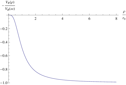
This (4.9) is indeed a monotonically decreasing function of $\rho$ , when viewing together with the coordinate redefinition (2.32). This can be easily understood if we notice following three facts: (i) $A_{t}^{\prime}(r)$ is a monotonically decreasing function of $r$ . (ii) The last factor in the integrand of (4.9) is the instanton density function which is peaked at $\tilde{r}=0$ and monotonically decreasing in $\tilde{r}$ , while the width of the function is given by $\rho$ and the function has a normalized integral (which is the instanton number). (iii) The map (2.32) between $r$ and $\tilde{r}$ is a one-to-one and monotonic function. The instanton modulus potential $V(\rho)$ (4.9) shows that the system dynamically favors the Higgs phase, $\rho\neq 0$ . This is the color-flavor locking in the supersymmetric QCD.

The $V_{B}(\rho)$ from the CS term computation (4.9) does not appear to be analytically integrable, however to get a qualitative understanding we can consider the following asymptotic values:

\displaystyle V_{B}(\rho=0)=0\,,\quad V_{B}(\rho=\infty)=-\frac{2\pi\alpha^{\prime}{\bf{d}}}{N_{c}}\int_{0}^{\infty}A_{t}^{\prime}dr=-\frac{2\pi\alpha^{\prime}{\bf d}\mu}{N_{c}}\,.

(4.10)

Their difference,

\displaystyle V_{B}(\rho=0)-V_{B}(\rho=\infty)=\frac{2\pi\alpha^{\prime}{\bf{d}}\mu}{N_{c}}

(4.11)

is consistent with the interpretation that we pull out one quark per each baryon to the infinity in the background chemical potential $\mu$ . However, note that the constant $F_{123}^{(3)}$ is obtained only in the vicinity of $r=0$ . So, our calculation is strictly valid only for small $\rho$ , and the potential height (4.11) derived at large $\rho$ should not be reliable. We however expect that the qualitative physical result (4.11) is not modified significantly when we taken into account of full $F_{123}^{(3)}$ at large radius. For completeness, here we include the plot of the one instanton size modulus potential, normalized by the asymptotic value $V_{B}(\infty)$ :

In the analysis above, we assumed that the center of the BPST instanton is at the origin. However, we can consider a generic situation where the center of the instanton is not at the origin $r=0$ . Suppose that the center is at some distance ${\bf X}$ from the origin. It is clear that the similar expression to (4.9), which is again only valid at small $r$ , would give a qualitative result that the potential $V_{B}(\rho,{\bf X})$ goes to its minimum at $(\rho,{\bf X})=(\infty,{\rm finite})$ or $(\rho,{\bf X})=({\rm finite},\infty)$ . The latter is in particular an extreme point in the moduli space in the Coulomb phase. There $\rho$ can vanish and in that case the color-flavor locking does not occur. However, for ${\bf X}\neq 0$ , the original gauge group $U(N_{c})$ is explicitly broken, as it is in the Coulomb phase.

Instead of substituting the BPST instanton, we can substitute multi-instanton solutions. Suppose we treat $\tilde{N}_{c}$ instantons. We need to require $\tilde{N}_{c}\ll N_{c}$ , because in the perturbation of the backreaction the original background of $AdS_{5}\times S^{5}$ should not be drastically modified. Generically, the instantons are separated from each other.¹¹¹¹ 11 Since electrically charged instantons should repel each other, generic configurations should be with the separated instantons. This phenomenon is common with the interaction among baryons [42] in the Sakai-Sugimoto model [43]; the repulsive core of nucleons is mainly due to this electric repulsion. Our analysis for the single BPST instanton holds also for the multi-instanton case. Then it is shown that all the size moduli of the instantons are destabilized.

4.3 What is Locked?

Naively speaking, the condensation of the squark field which comes from a fluctuation of a string connecting the D3-branes and the D7-branes gives the instanton size. This string transforms in the fundamental representation of the gauge group $U(\tilde{N}_{c})$ and in the anti-fundamental representation of the flavor group¹²¹² 12 Precisely speaking, the flavor group of the supersymmetric QCD should be $SU(N_{f})$ , since the overall $U(1)$ transformation of the flavor symmetry can be identified as a global part of a $U(1)$ subgroup of the local gauge group. In the following, we adopt $U(N_{f})$ rather than $SU(N_{f})$ , but the argument goes similarly. $U(N_{f})$ . Here $U(\tilde{N}_{c})$ is a part of the total gauge group $U(N_{c})$ i.e. $\tilde{N}_{c}\leq N_{c}$ . The partial color symmetry is for our convenience to consider $\tilde{N}_{c}$ instantons only to dissolve into the worldvolume of the D7-branes. By the squark condensation, apparently the color and the flavor symmetries $U(\tilde{N}_{c})\times U(N_{f})$ are broken. We shall see the symmetry breaking pattern.

The theory on the instantonic D3-branes is constructed from their ADHM data [30]. The ADHM data consists of four $U(\tilde{N}_{c})$ adjoint scalar fields which are combined into two $\tilde{N}_{c}\times\tilde{N}_{c}$ complex scalar fields $B_{1}$ and $B_{2}$ , and the squark fields $I^{\dagger}$ and $J$ which are complex $N_{f}\times\tilde{N}_{c}$ matrix scalar fields. The squark fields transform as

\displaystyle I^{\dagger}\mapsto UI^{\dagger}U_{0}^{-1},\quad J\mapsto UJU_{0}^{-1},

(4.12)

where $U\in U(N_{f})$ and $U_{0}\in U(\tilde{N}_{c})$ . So these fields are in the bi-fundamental representation.

Let us consider ’t Hooft instantons. Then $B_{1}$ and $B_{2}$ are diagonal matrices, and the ADHM equations are nothing but the BPS equations for the theory on the D3-branes, are

\displaystyle II^{\dagger}=J^{\dagger}J\,,\quad IJ=0\,.

(4.13)

This of course allows a trivial solution $I^{\dagger}=J=0$ , which corresponds to the zero-size instanton.

First we consider the two-flavor case $N_{f}=2$ . The flavor symmetry is $U(2)$ which is a vector part of the chiral symmetry (the chiral symmetry is explicitly broken by the quark/squark mass in our case). The ’tHooft instanton whose centers are located at the origin is represented by a solution

\displaystyle I^{\dagger}=\left(\begin{array}[]{cccc}\rho_{1}&\rho_{2}&\cdots&\rho_{\tilde{N}_{c}}\\ 0&0&\cdots&0\end{array}\right),\quad J=\left(\begin{array}[]{cccc}0&0&\cdots&0\\ \rho_{1}&\rho_{2}&\cdots&\rho_{\tilde{N}_{c}}\end{array}\right).

Here, all $\rho_{i}$ ’s are real parameters. These correspond to size of each instanton. With this at hand, we can compute unbroken symmetry.

For simplicity, we consider the case of a single instanton, $\tilde{N}_{c}=1$ .

\displaystyle I^{\dagger}=\rho\left(\begin{array}[]{cccc}1\\ 0\end{array}\right),\quad J=\rho\left(\begin{array}[]{cccc}0\\ 1\end{array}\right).

Here $\rho$ is a nonzero constant (for which we computed the potential). In this case, the transformation which leaves $I^{\dagger}$ intact is

\displaystyle U=\left(\begin{array}[]{cc}e^{i\alpha_{1}}&0\\ 0&e^{i\alpha_{2}}\end{array}\right),\quad U_{0}=e^{i\alpha_{1}},\quad\alpha_{i}\in{\mathbb{R}}\,.

On the other hand, the symmetry which leaves $J$ intact is

\displaystyle U=\left(\begin{array}[]{cc}e^{i\alpha_{1}}&0\\ 0&e^{i\alpha_{2}}\end{array}\right),\quad U_{0}=e^{i\alpha_{2}},\quad\alpha_{i}\in{\mathbb{R}}\,.

Therefore, we need to require $\alpha_{1}=\alpha_{2}$ , and we conclude,

\displaystyle U(1)_{\rm color}\times U(2)_{\rm flavor}\to U(1)_{\rm CFL}\,.

(4.30)

The global part of $U(1)_{\rm color}$ is locked with the diagonal part of $U(2)_{\rm flavor}$ , which is the baryonic symmetry $U(1)_{B}$ , and the local part of $U(1)_{\rm color}$ is broken.

This kind of the color-flavor locking can be found for general $N_{f}$ . In the case of $\tilde{N}_{c}=1$ , the squark condensations are given by

\displaystyle I^{\dagger}=\rho\left(\begin{array}[]{cccc}1\\ 0\\ 0\\ \vdots\\ 0\end{array}\right),\quad J=\rho\left(\begin{array}[]{cccc}0\\ 1\\ 0\\ \vdots\\ 0\end{array}\right).

A similar analysis shows

\displaystyle U(1)_{\rm color}\times U(N_{f})_{\rm flavor}\to U(1)_{\rm CFL}\times U(N_{f}-2)_{\rm flavor}\,.

(4.42)

$U(1)_{\rm CFL}$ is a global symmetry which locks a part of the flavor symmetry and the gauge symmetry. Note that for $N_{f}>2$ , this $U(1)_{\rm CFL}$ can be nothing to do with the baryonic symmetry $U(1)_{B}$ , since the action of this $U(1)_{\rm CFL}$ can be chosen as

\displaystyle U=\mbox{diag}(e^{i\alpha},e^{i\alpha},e^{-2i\alpha/N_{f}},\cdots,e^{-2i\alpha/N_{f}}),\quad U_{0}=e^{i\alpha},\quad\alpha\in{\mathbb{R}}\,.

(4.43)

For generic $\tilde{N}_{c}$ , we expect that all the size moduli are driven to have nonzero values (for example, for $N_{f}=2$ we have (4.3)). So the symmetry is broken as

\displaystyle U(\tilde{N}_{c})_{\rm color}\times U(N_{f})_{\rm flavor}\to U(1)_{\rm CFL}\times U(N_{f}-2)_{\rm flavor}\,.

(4.44)

The locking is quite similar to the case of $\tilde{N}_{c}=1$ . Note that we restrict ourselves to the case of the ’tHooft instantons. Since the ’tHooft instantons do not cover all the moduli space of the instantons, there remains a possibility that the unbroken symmetry, in particular the part concerning the gauge symmetry, may be enhanced.

In the D-brane analysis, we used the technique for Coulomb branch in AdS/CFT correspondence and treat one D3-brane as a probe by separating it from the rest, by hand. This procedure for the separation is somewhat artificial, but it is required for the geometry not to be drastically modified by a possible back reaction, which is our limitation.

5 Extension to Finite Temperature System

In this section we explore the system at finite temperature and baryon density. Since the boundary geometry of our $AdS_{5}\times S^{5}$ is $R^{1,3}$ , the geometry creates a horizon inside $AdS$ at any finite temperature. ${\cal N}=4$ SYM theory coupled with ${\cal N}=2$ hypermultiplets in fundamental representation at finite temperature has been studied (See [44] for a review). As mentioned in Sec. 1, there are two brane embeddings in the black hole background: the Minkowski embedding and the black hole embedding (Fig. 2). The former describes the configuration of D-branes staying outside of the horizon everywhere and the latter describes the configuration of D-branes falling into the black hole horizon. The equations of motion and the free energy determine which configuration is realized at given quark mass and baryon density normalized by temperature: $m/T$ and $2\pi\alpha^{\prime}{\bf d}/T^{3}$ .

In the case of zero baryon density and no instanton, the Minkowski embedding covers only higher $m/T$ region while the black hole embedding covers only lower $m/T$ region [26]. These two are connected by a first order phase transition at certain critical temperature $(m/T)_{\rm crit.}$ . This phase transition is interpreted in the field theory as meson melting: the spectrum is discrete and the mesons are stable in the Minkowski embedding, while the spectrum is continuous and the mesons are unstable in the black hole embedding. In the case of finite baryon density, the Minkowski embedding is no longer physically allowed and the black hole embedding covers the whole temperature region. When an instanton is excited on the D7-branes at zero baryon density, the potential for the instanton size moduli takes its minimum at the origin, $\rho=0$ , for the Minkowski embeddings and at some finite value, $\rho=\rho_{\rm min}>0$ , for the black hole embeddings [35]. This means the system is in Higgs phase above the critical temperature $(m/T)_{\rm crit.}$ . Therefore, the system is already in a CFL phase with the squark condensation, in the melted meson phase with finite $T$ .

The purpose of this section is to study the case with both the finite baryon density and the instanton configuration. As we saw in the zero temperature case, the backreaction of the baryon density excites an additional CS term which induces the CFL. We will see how this CS term affects the instanton potential in the finite temperature system.

5.1 The D3D7 System at Finite Baryon Density and Temperature

The background geometry dual to the finite temperature system is an AdS black hole. In Poincare like coordinates, the metric, RR 4-form and the dilaton have the following expressions, in the conventions of Ref. [13]:

	$\displaystyle ds^{2}$	$\displaystyle=$	$\displaystyle{1\over 2}{u^{2}\over R^{2}}\left(-{f^{2}\over\widetilde{f}}dt^{2}+\widetilde{f}dx_{3}^{2}\right)+{R^{2}\over u^{2}}\left(du^{2}+u^{2}ds_{5}^{2}\right)$		(5.1)
	$\displaystyle C$	$\displaystyle=$	$\displaystyle{1\over R^{4}}\left({u^{2}\over 2}+{u^{4}_{0}\over 2u^{2}}\right)^{2}d^{4}x\,,~~~~~~e^{\Phi}=e^{\Phi_{0}}\,,$		(5.2)

where

\displaystyle f=1-{u_{0}^{4}\over u^{4}}\,,~~~\widetilde{f}=1+{u_{0}^{4}\over u^{4}}\,,

(5.3)

with $u_{0}$ the location of the horizon. $u$ and $r_{6}$ in Sec. 3 are related to each other by the coordinate transformation

\displaystyle u^{2}=r_{6}^{2}+\sqrt{r_{6}^{4}-u^{4}_{0}}\,.

(5.4)

The regularity of the Euclidean section of this geometry relates the horizon radius $u_{0}$ and the Hawking temperature, which is interpreted as a temperature of the boundary gauge theory of our concern, as

\displaystyle T={u_{0}\over\pi R^{2}}\,.

(5.5)

As in the zero temperature case, we foliate $S^{5}$ with $S^{3}$ so that $SO(3)$ R-symmetry is manifest:

\displaystyle du^{2}+u^{2}ds_{5}^{2}

\displaystyle=

\displaystyle du^{2}+u^{2}(d\theta^{2}+\sin^{2}{\theta}ds^{2}_{3}+\cos^{2}\theta d\phi^{2})\,,

(5.6)

where $\theta,\phi$ and $\theta_{1},\theta_{2}$ in (3.8) are related through the following equations

\displaystyle\sin\theta=\sin\theta_{1}\sin\theta_{2}\,,~~~~~\tan\phi={\cos\theta_{1}\over\sin\theta_{1}\cos\theta_{2}}\,.

(5.7)

The probe D7-brane worldvolume is spanned by $(t,x^{i},u,S^{3})$ , and is localized in $\phi$ direction, which we can use rotational symmetry to set $\phi=0$ (corresponding to $\theta_{1}=\frac{\pi}{2}$ ). In the new coordinates, the embedding is described by $\chi\equiv\cos\theta$ as a function of $u$ . The $U_{b}(1)$ gauge field $A$ dual to the baryon current on the boundary has only non-zero time component

\displaystyle A=A_{t}(u)dt.

(5.8)

With these ansätze, the DBI action of the D7-branes is given by

	$\displaystyle\frac{S_{\rm DBI}^{\rm D7}}{V_{4}}$	$\displaystyle=$	$\displaystyle\int\!du\;{\mathcal{L}}$		(5.9)
		$\displaystyle=$	$\displaystyle-{\cal N}\int\!du\;{u^{3}f\tilde{f}(1-\chi^{2})\over 4}\sqrt{1-\chi^{2}+u^{2}\dot{\chi}^{2}-(2\pi{\alpha^{\prime}}\dot{A_{t}})^{2}{2\tilde{f}(1-\chi^{2})\over f^{2}}}$		(5.10)

where the dot denotes ${d\over du}$ and ${\cal N}$ is as defined below (2.8). Since the action does not contain $A$ explicitly, the momentum conjugate of $A$ is constant:

\displaystyle{\delta{\mathcal{L}}\over\delta(2\pi{\alpha^{\prime}}\dot{A}_{t})}={\cal N}{u^{3}\over 2}{\tilde{f}^{2}\over f}{(1-\chi^{2})^{2}(2\pi{\alpha^{\prime}}\dot{A}_{t})\over\sqrt{1-\chi^{2}+u^{2}\dot{\chi}^{2}-(2\pi{\alpha^{\prime}}\dot{A_{t}})^{2}{2\tilde{f}(1-\chi^{2})\over f^{2}}}}\equiv{\bf D}\,,

(5.11)

or equivalently,

\displaystyle 2\pi{\alpha^{\prime}}\dot{A}=2\left({{\bf D}\over{\cal N}}\right){f\sqrt{1-\chi^{2}+u^{2}\dot{\chi}^{2}}\over\sqrt{\tilde{f}(1-\chi^{2})}\sqrt{u^{6}\tilde{f}^{3}(1-\chi^{2})^{3}+8({\bf D}/{\cal N})^{2}}}\,.

(5.12)

To derive the equation of motion for $\chi$ , we Legendre transform the action with respect to ${\bf D}$ so that $\dot{A}_{t}$ can be eliminated from the action:

	$\displaystyle\tilde{{\mathcal{L}}}$	$\displaystyle=$	$\displaystyle{\mathcal{L}}-{\delta L\over\delta(2\pi{\alpha^{\prime}}\dot{A}_{t})}(2\pi{\alpha^{\prime}}\dot{A}_{t})$		(5.13)
		$\displaystyle=$	$\displaystyle-{{\cal N}\over 4}{f\over\sqrt{\tilde{f}}\sqrt{1-\chi^{2}}}\sqrt{1-\chi^{2}+u^{2}\dot{\chi}^{2}}\sqrt{u^{6}\tilde{f}^{3}(1-\chi^{2})^{3}+8({\bf D}/{\cal N})^{2}}\,.$		(5.14)

Then the $\chi$ equation is

	$\displaystyle\partial_{u}\left({u^{5}f\tilde{f}(1-\chi^{2})\dot{\chi}\over\sqrt{1-\chi^{2}+u^{2}\dot{\chi}^{2}}}\sqrt{1+{8({\bf D}/{\cal N})^{2}\over u^{6}\tilde{f}^{3}(1-\chi^{2})^{3}}}\right)$		(5.15)
	$\displaystyle\quad=-{u^{3}f\tilde{f}\chi\over\sqrt{1-\chi^{2}+u^{2}\dot{\chi}^{2}}}\sqrt{1+{8({\bf D}/{\cal N})^{2}\over u^{6}\tilde{f}^{3}(1-\chi^{2})^{3}}}$		(5.16)
	$\displaystyle\quad\quad\times\left(3(1-\chi^{2})+2u^{2}\dot{\chi}^{2}-24\left({{\bf D}\over{\cal N}}\right)^{2}{1-\chi^{2}+u^{2}\dot{\chi}^{2}\over u^{6}\tilde{f}^{3}(1-\chi^{2})^{3}+8({\bf D/{\cal N}})^{2}}\right).$		(5.17)

As studied in Ref. [45], the boundary condition of probe branes at the horizon is determined by the regularity of the induced curvature: $\dot{\chi}|_{u=u_{0}}=0$ . With this boundary condition, the solution of this equation of motion near the horizon $u\sim u_{0}$ is then given by

\displaystyle\chi=\chi_{0}-{3\chi_{0}(1-\chi_{0}^{2})^{3}\over 4(({\bf D}^{2}/{\cal N}^{2}u_{0}^{3})+1-\chi^{6}_{0}-3\chi_{0}^{2}(1-\chi^{2}_{0}))}\left(\!{u\over u_{0}}\!-\!1\!\right)^{2}\!+{\mathcal{O}}\left(\!\left({u\over u_{0}}\!-\!1\right)^{3}\right)\,.

(5.18)

Therefore, the embedding can be approximated as

\displaystyle\chi=\chi_{0},~~~\dot{\chi}=0,

(5.19)

for ${u\over u_{0}}-1$ smaller than ${2\over\sqrt{3}(1-\chi_{0}^{2})^{3/2}}{{\bf D}\over{\cal N}u_{0}^{3/2}}$ with large ${\bf D}$ .

We again consider the instanton excitations as a perturbation in this background field. At the leading order of ${\bf D}/N_{c}$ , the instanton couples to RR 4-form and the induced metric, and the relevant terms are:

\displaystyle S_{\rm DBI}^{\rm D7}(FF)

\displaystyle=

\displaystyle-N_{f}{\cal T}_{\rm D7}\int d^{4}x\int{u^{4}\over 4R^{4}}f\widetilde{f}\cdot{(2\pi\alpha^{\prime})^{2}\over 8}\mathop{\rm Tr}\nolimits[F\wedge F]\,,

(5.20)

\displaystyle S_{\rm CS}^{\rm D7}(FF)=N_{f}{\cal T}_{\rm D7}\int d^{4}x\int{u^{4}\over 4R^{4}}\tilde{f}^{2}\cdot{(2\pi\alpha^{\prime})^{2}\over 8}\mathop{\rm Tr}\nolimits[F\wedge F]\,.

(5.21)

The instanton $F\wedge F$ lives on an effective four dimensional space whose metric is

	$\displaystyle\widetilde{G}^{4}_{ij}$	$\displaystyle=$	$\displaystyle\left({1\over 2}\sqrt{f\widetilde{f}}\right)\left(\left({1-\chi^{2}+u^{2}\dot{\chi}^{2}\over 1-\chi^{2}}+{(2\pi\alpha^{\prime})^{2}\dot{A}^{2}\over-{1\over 2}{f^{2}\over\widetilde{f}}}\right)du^{2}+u^{2}(1-\chi^{2})ds_{3}^{2}\right)$		(5.22)
		$\displaystyle=$	$\displaystyle{\sqrt{f\widetilde{f}}\over 2}\left(\left(1+{u^{2}\dot{\chi}^{2}\over 1-\chi^{2}}\right){u^{6}\tilde{f}^{3}(1-\chi^{2})^{3}\over u^{6}\tilde{f}^{3}(1-\chi^{2})^{3}+8({\bf D}/{\cal N})^{2}}du^{2}+u^{2}(1-\chi^{2})ds_{3}^{2}\right)\,.$		(5.22)

Note that ${\bf D}$ dependence appears only through this metric. The difference between the DBI term and the CS term is the factors of $f$ and $\tilde{f}$ in the integrands. Therefore, the instanton potential vanishes as long as the temperature is zero, even in the presence of finite baryon density as we have seen.

5.2 CS Term from Backreaction

The next leading order in ${\bf D}/N_{c}$ comes from the backreaction of the gauge field to RR fields. Similar calculations show that it excites the same constant RR 3-form field near the horizon as that of the zero temperature case with ${\bf d}$ replaced by ${\bf D}$ ,

\displaystyle F^{(3)}_{123}={8\pi^{3}{\alpha^{\prime}}^{2}{\bf D}\over N_{c}}\,.

(5.24)

Therefore it induces the same CS term

\displaystyle S_{\rm CS}^{\rm D7}({\bf{D}})={{\alpha^{\prime}}{\bf D}\over 16\pi N_{c}}\int d^{4}x\int\mathop{\rm tr}\nolimits\left[A\wedge F\wedge F\right].

(5.25)

The remaining issue is to obtain the explicit instanton configuration $\mathop{\rm tr}\nolimits\left[F\wedge F\right]$ on the effective metric $\widetilde{G}_{ij}^{(4)}$ . As in the zero temperature case, we would like to obtain a conformally flat coordinate $\widetilde{u}$ satisfying:

\displaystyle\widetilde{G}_{ij}^{(4)}=S(\widetilde{u})^{2}(d\widetilde{u}^{2}+\widetilde{u}^{2}ds_{3})\,.

(5.26)

For the approximate embedding near the horizon (5.19), the conformally flat metric (5.26) is obtained by

\displaystyle{u^{2}(1-\chi_{0}^{2})\sqrt{\tilde{f}}\over\sqrt{u^{6}\tilde{f}^{3}(1-\chi^{2}_{0})^{3}+8({\bf D}/{\cal N})^{2}}}du={d\tilde{u}\over\tilde{u}}\,.

(5.27)

With this conformally flat coordinate, the BPST instanton is given by

\displaystyle\mathop{\rm tr}\nolimits\left[F\wedge F\right]={192\rho^{4}\over(\widetilde{u}^{2}+\rho^{2})^{4}}d^{4}\widetilde{\xi}\,.

(5.28)

As we have seen, there are three terms contributing the instanton potential for the finite temperature case: the DBI and the CS term for thermal effect, which we denote $V_{T}$ , and the CS term from the backreaction, which we denoted earlier as $V_{B}$ . From (5.20) and (5.21), the thermal potential is

	$\displaystyle V_{T}(\rho)$	$\displaystyle=$	$\displaystyle-(S_{\rm DBI}^{\rm D7}(FF)+S_{\rm CS}^{\rm D7}(FF))/V_{4}$		(5.29)
		$\displaystyle=$	$\displaystyle-{{\cal N}\over 4R^{4}}\int\!d\widetilde{u}\;u^{4}\widetilde{f}(\widetilde{f}-f)\cdot{(2\pi\alpha^{\prime})^{2}\over 8}{192\rho^{4}\tilde{u}^{3}\over(\widetilde{u}^{2}+\rho^{2})^{4}}\,.$		(5.30)

This potential has a minimum at finite $\rho$ since $V_{T}(0)=V_{T}(\infty)=0$ . On the other hand, from (5.25), the potential from the backreaction is

	$\displaystyle V_{B}(\rho)$	$\displaystyle=$	$\displaystyle-S_{\rm CS}^{\rm D7}({\bf D})/V_{4}$		(5.31)
		$\displaystyle=$	$\displaystyle-{{\bf D}^{2}\over N_{c}{\cal N}}\int_{u=u_{0}}du{2f\over\sqrt{\tilde{f}}\sqrt{u^{6}\tilde{f}^{3}(1-\chi_{0}^{2})^{3}+8({\bf D}/{\cal N})^{2}}}{\rho^{4}(3\widetilde{u}^{2}+\rho^{2})\over(\widetilde{u}^{2}+\rho^{2})^{3}}\,.$		(5.32)

The approximation we used to obtain the integrands breaks down for large $u$ . However, the following two features may still hold even beyond the approximation: $V_{B}(0)=0$ and $V_{B}(\infty)=-{(2\pi{\alpha^{\prime}}){\bf D}\mu\over N_{c}}$ . The first one, $V_{B}(0)=0$ , comes from the fact that the integration of the instanton term, the last term in (5.32), is zero for $\rho=0$ . Therefore, independent of the form of $F_{3}$ and $\dot{A}_{t}$ , the integration gives zero. The second one, $V_{B}(\infty)=-{(2\pi{\alpha^{\prime}}){\bf D}\mu\over N_{c}}$ , comes from the physical reason explained in Section 4.2 for the zero temperature case. A numerical analysis suggests that $V_{B}$ monotonically decreases from zero to $-{(2\pi{\alpha^{\prime}}){\bf D}\mu\over N_{c}}$ .

The shape of the total potential $V=V_{T}+V_{B}$ then depends on the ratio between them, which is characterized by

\displaystyle{V_{B}\over V_{T}}\sim{g_{s}\over 12\pi}{1\over u_{0}^{4}}\left({{\bf D}\over{\cal N}}\right)^{{4\over 3}}.

(5.33)

Physically, this suggests that the thermal effect dominates when the temperature is high (large $u_{0}$ ), while the backreaction effect dominates when the baryon density is high (large ${\bf D}$ ).¹³¹³ 13 Note that both potentials are of ${\cal O}(1/N_{c})$ for fixed $g_{s}$ ( $\sim$ fixed ratio of $\lambda/N_{c}$ ). Note that $\left({{\bf D}/{\cal N}}\right)$ can be large up to the order of $(N_{c}/N_{f})$ where the probe flavor brane description breaks down. Therefore, the ratio $(V_{B}/V_{T})$ may become large despite the fact that it is a positive power of $g_{s}$ . Recalling that $V_{T}$ has a local stable minimum and $V_{B}$ is a run-away type potential, we conclude that the potential can have three possible behaviors depending on the ratio between ${\bf D}$ and $u_{0}$ . When $(({\bf D}/{\cal N})^{4/3}/u_{0}^{4})$ is very small, $V_{T}$ dominates the potential and it has a local stable minimum. The size of the instanton in this case is about the order of the horizon scale. Since observables which have less energy than the temperature have no meaning at finite temperature, the finiteness of the instanton size may be interpreted as a thermal effect. As $(({\bf D}/{\cal N})^{4/3}/u_{0}^{4})$ increases, the local minimum becomes a meta-stable state and the instanton size $\rho$ eventually decays to infinity. As $(({\bf D}/{\cal N})^{4/3}/u_{0}^{4})$ increases further, $V_{B}$ dominates the potential and the local minimum disappears. These features are shown in Figure 6.

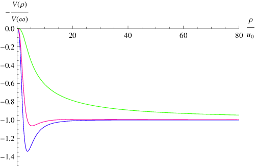
Thermal quantities such as the derivative of the free energy may change discontinuously at a critical value of $(({\bf D}/{\cal N})^{4/3}/u_{0}^{4})$ . Therefore, this shows a phase transition within the CFL phase. For larger temperature, we have a CFL phase with the finite size instanton, while for larger baryon density, we have another CFL phase with the size of the instanton being very large. A schematic picture of the phase diagram is shown in Fig. 3.

As in the case of $T=0$ , our analysis is valid only for small $u$ region and cannot say anything precise about the potential at large $u$ . From the boundary theory point of view, the stability at higher temperature may be understood as the thermal masses of the scalar fields and the instability at higher density may be understood as the tachyonic masses of the scalar fields from the chemical potential. Since the supersymmetry is completely broken, the potential might be lifted up by cubic and higher terms and the vevs of the squarks may take finite values. Of course, these expectations are from the weak coupling analysis of the gauge theory and the strong coupling dynamics might change the picture. We do not go into the detail on this point in this paper.

6 Discussions

In this paper, we made some preliminary steps towards a holographic model of color-flavor locking phase, here we end with a list of interesting future directions which seem worth exploring.

The phase diagram (Fig. 3) is obtained by the total potential $V_{T}+V_{B}$ for the instanton size modulus, but the potential $V_{B}$ is valid only for a restricted region for $r$ , as shown in Sec. A. So, it is important to compute the backreaction which is valid in all region of $r$ , to explore the phase diagram further.

In particular for $T=0$ , we have shown that there is an instability along the direction of squark VEV in the melted meson phase. This means that the critical chemical potential dividing the meson and melted meson phases may take a different value which is smaller than $\mu=m$ . Our method of treating $\tilde{N}_{c}$ D3-branes among $N_{c}$ of them separately cannot reach the true value of the critical chemical potential in the full phase diagram, and this deserves a further study. It is possible that there may be no vacuum if the potential valid for all $r$ is found and turns out to be a run-away type. See [46] for a related discussion for R-charge chemical potential.

A related issue is a possible distinction between the two CFL Higgs phases. We have two CFL phases, one is with finite instanton size $\rho$ while the other is with $\rho=\infty$ . The former is realized mainly by the thermal potential for $\rho$ , while the latter is by a domination of the baryon density. The symmetry breaking patterns look similar to each other. However, we expect that, once the repulsion among electrically charged instantons is included, the remaining symmetries may differ. In addition, physical solitonic spectra in these CFL vacua may be different from each other. It would be interesting to study vortex strings in these vacua.

The vortex strings in the CFL phase in QCD play important roles in various physics (see Ref. [47] for a partial list of related papers), and the D-brane techniques for the CFL phase studied in this paper may be helpful in revealing the properties of those vortex strings. Since the vortex strings are inside the D3-branes which are instantons on the D7-branes, this suggests that “vortices inside instantons” are possible. This is intriguing on its own in soliton physics.

It was described in Ref. [48] that in an idealistic situation the CFL phase of QCD may be continuously connected to the hadron phase, giving a continuous deformation of the excitation spectrum, named “quark-hadron continuity”. In our case, the dynamically favored CFL phase is in the melted meson phase, so the fluctuation spectrum is continuous, which means that the spectral “continuity” doesn’t make much sense. However, in our ${\cal N}=4$ YM theory coupled to the ${\cal N}=2$ quark hypermultiplet, it is known that the meson phase is continuously connected to a Higgs phase [31]. This marginal deformation does not cost any energy, and the baryon number density is kept to be zero. The instanton size modulus is a free parameter (that is, the squark VEV is a flat direction of the theory). In this deformation, it was shown in Ref. [32] that the discrete fluctuation spectrum is smoothly deformed. See Fig. 1 of Ref. [32]. This phenomenon is analogous to the spectral quark-hadron continuity.

It is well-known that color-flavor locking phase in QCD closely resembles the locking between spin and orbital symmetries found in the so-called “B-phase” of superfluid Helium 3, the setup we consider here therefore seems to be directly applicable in realizing this in string theory. One can study various thermodynamical properites and also consider topological defects e.g. vortices and study in such phase. Some interesting work relating D3D7 system with fermi-liquid can be found in Refs. [49].

Finally, it would be interesting to study a possible universality of the CFL at finite baryon density among holographic models. In the D4/D6 system considered in Ref. [29], the dual field theory becomes effectively a pure bosonic Yang-Mills theory at low energy [50]. The phase structure of this system at finite temperature and baryon density was shown to have universal properties in Ref. [37]. Therefore, it is expected that when the baryon number density increases, the system becomes unstable and some of the D4-branes would be pulled onto the D6 branes. In this case, the squarks condensation corresponds to an expansion of monopoles on the D6-branes, instead of the instantons. As mentioned in Sec. 3.1, in the deconfinement phase, the baryon vertex is replaced by a flux while there is no probe brane description[38]. On the other hand, in a confining phase, the baryon vertex does have a probe brane description, and the discussion in Sec. 3.1 at zero temperature does not apply to the case. Therefore, it would be interesting to investigate the possibility of CFL in a confinement phase.

Acknowledgments.

We would like to thank Johanna Erdmenger, Aki Hashimoto, Deog-Ki Hong, Elias Kiritsis, Shin Nakamura, Hirosi Ooguri, Shigeki Sugimoto and Seiji Terashima for discussions. We would also like to thank Rob Myers and David Mateos for giving many useful comments on the draft. K.H. thanks Kavli Institute for Theoretical Physics at UCSB for providing an ideal environment for discussions, and thanks Aki Hashimoto for kind hospitality to support his visit to the physics department at University of Wisconsin. He also thanks the Yukawa Institute for Theoretical Physics at Kyoto University, at which this topic was discussed during the workshop YITP-W-09-04 on “Development of Quantum Field Theory and String Theory.” HYC is supported in part by NSF CAREER Award No. PHY-0348093, DOE grant DE-FG-02-95ER40896, a Research Innovation Award and a Cottrell Scholar Award from Research Corporation, and a Vilas Associate Award from the University of Wisconsin. KH. is partly supported by the Japan Ministry of Education, Culture, Sports, Science and Technology. The work of SM is supported in part by National Science Foundation under grant No. PHY05-51164 and Japan Society for the Promotion of Science.

Appendix A Check of Consistency for the Linearized Perturbation

To complete the analysis of Sec. 3.2, we shall now check if this can be regarded as a small backreaction, so that our perturbative treatment for solving the equations of motion of the supergravity is guaranteed. The second term of (3.13) suggests that the nonzero $F_{3}$ (3.1) will again backreact the $F_{5}$ flux. We examine that this backreaction does not spoil the original flux configuration (2.3) too much. To this end, we compare the second term of (3.13) with the $F_{5}$ kinetic term

\displaystyle\frac{-1}{8\kappa_{10}^{2}}\int\!d^{10}x\sqrt{-g_{10}}|F_{5}|^{2}.

(A.1)

We are only interested in order of magnitudes. Solving (3.17), we obtain

\displaystyle B_{0r_{6}}\sim r_{6}^{-3}g_{s}^{2}\alpha^{\prime 4}{\bf{d}}\,.

(A.2)

Using this and (3.1) (2.3), we evaluate the second term of (3.13) as

\displaystyle\frac{1}{4\kappa_{10}^{2}}\int F_{5}\wedge B_{2}\wedge F_{3}\sim\int d^{4}xdr_{6}d\Omega_{5}\;r_{6}^{-3}g_{s}^{2}\alpha^{\prime 4}{\bf{d}}^{2}\,.

(A.3)

On the other hand, the $F_{5}$ kinetic term (A.1) with the flux solution (2.3) gives

\displaystyle\frac{-1}{8\kappa_{10}^{2}}\int\!d^{10}x\sqrt{-g_{10}}|F_{5}|^{2}\sim\int d^{4}xdr_{6}d\Omega_{5}\;r_{6}^{3}g_{s}^{-2}\alpha^{\prime-4}\,.

(A.4)

Requiring (A.3) being much smaller than (A.4), we obtain

\displaystyle g_{s}^{4}\alpha^{\prime 8}{\bf{d}}^{2}\ll r_{6}^{6}\,.

(A.5)

This means that, for the backreaction to the 5-form flux $F_{5}$ to be small, we need to work in this region for $r_{6}$ .

On the other hand, we made the assumption $r\ll r_{0}$ to simplify the source term to get (3.12). Around the tip, we have a relation $r_{6}^{2}=r^{2}+y(r)^{2}\sim r^{2}(1+y^{\prime}(0))$ , so this assupmtion translates to the condition $r_{6}^{2}({\bf{d}}^{2}-{\bf{c}}^{2})/{{\bf{d}}^{2}}\ll r_{0}^{2}$ which is equivalent to

\displaystyle r_{6}^{6}\ll\alpha^{\prime 8}g_{s}^{2}N_{f}^{-2}{\bf{d}}^{6}/({\bf{d}}^{2}-{\bf{c}}^{2})^{2}\,.

(A.6)

Therefore, in order to have a region for $r_{6}$ which satisfies the two requirements (A.5) and (A.6), we need

\displaystyle g_{s}N_{f}\ll{\bf{d}}^{2}/({\bf{d}}^{2}-{\bf{c}}^{2})\,.

(A.7)

With (2.16) and (2.17), this condition is met if we are close to the critical chemical potential,

\displaystyle\mu-m\ll\mu\,,m\,.

(A.8)

Throughout this paper, we are working in this regeme.

Note that when ${\bf{d}}^{2}-{\bf{c}}^{2}\ll{\bf{d}}^{2}$ with which (A.7) is satisfied, the D7-brane spike becomes very narrow, and the spike can be well-approximated by fundamental strings. This means that dilaton backreaction can be safely neglected. The backreaction to the metric is suppressed by $1/N_{c}$ and also neglected.

References

[1]

K. Rajagopal and F. Wilczek, “The condensed matter physics of QCD,” arXiv:hep-ph/0011333.

M. G. Alford, A. Schmitt, K. Rajagopal and T. Schafer, “Color superconductivity in dense quark matter,” Rev. Mod. Phys. 80, 1455 (2008) [arXiv:0709.4635 [hep-ph]].
[2] J. M. Maldacena, “The large N limit of superconformal field theories and supergravity,” Adv. Theor. Math. Phys. 2, 231 (1998) [Int. J. Theor. Phys. 38, 1113 (1999)] [arXiv:hep-th/9711200].
[3]

S. S. Gubser, I. R. Klebanov and A. M. Polyakov, “Gauge theory correlators from non-critical string theory,” Phys. Lett. B 428, 105 (1998) [arXiv:hep-th/9802109].

E. Witten, “Anti-de Sitter space and holography,” Adv. Theor. Math. Phys. 2, 253 (1998) [arXiv:hep-th/9802150].

O. Aharony, S. S. Gubser, J. M. Maldacena, H. Ooguri and Y. Oz, “Large N field theories, string theory and gravity,” Phys. Rept. 323, 183 (2000) [arXiv:hep-th/9905111].
[4]

E. Witten, “Baryons and branes in anti de Sitter space,” JHEP 9807, 006 (1998) [arXiv:hep-th/9805112].

Y. Imamura, “Supersymmetries and BPS configurations on Anti-de Sitter space,” Nucl. Phys. B 537, 184 (1999) [arXiv:hep-th/9807179].

C.G. Callan, A. Guijosa and K.G. Savvidy, “Baryons and string creation from the fivebrane worldvolume action,” Nucl. Phys. B 547, 127 (1999) [arXiv:hep-th/9810092].

B. Craps, J. Gomis, D. Mateos and A. Van Proeyen, “BPS solutions of a D5-brane worldvolume in a D3-brane background from superalgebras,” JHEP 9904, 004 (1999) [arXiv:hep-th/9901060].

C.G. Callan, A. Guijosa, K.G. Savvidy and O. Tafjord, “Baryons and flux tubes in confining gauge theories from brane actions,” Nucl. Phys. B 555 (1999) 183 [arXiv:hep-th/9902197].
[5] D. J. Gross and H. Ooguri, “Aspects of large N gauge theory dynamics as seen by string theory,” Phys. Rev. D 58, 106002 (1998) [arXiv:hep-th/9805129].
[6]

F. Benini, F. Canoura, S. Cremonesi, C. Nunez and A. V. Ramallo, “Unquenched flavors in the Klebanov-Witten model,” JHEP 0702, 090 (2007) [arXiv:hep-th/0612118].

F. Benini, F. Canoura, S. Cremonesi, C. Nunez and A. V. Ramallo, “Backreacting Flavors in the Klebanov-Strassler Background,” JHEP 0709, 109 (2007) [arXiv:0706.1238 [hep-th]].

R. Casero, C. Nunez and A. Paredes, “Elaborations on the String Dual to N=1 SQCD,” Phys. Rev. D 77, 046003 (2008) [arXiv:0709.3421 [hep-th]].
[7]

R. Harnik, D. T. Larson and H. Murayama, “Supersymmetric color superconductivity,” JHEP 0403, 049 (2004) [arXiv:hep-ph/0309224].

N. Maru and M. Tachibana, “Color superconductivity from supersymmetry,” Mod. Phys. Lett. A20, 1495 (2005) [arXiv:hep-ph/0411079].
[8] D. V. Deryagin, D. Y. Grigoriev and V. A. Rubakov, “Standing wave ground state in high density, zero temperature QCD at large N(c),” Int. J. Mod. Phys. A 7, 659 (1992).
[9]

E. Shuster and D. T. Son, “On finite-density QCD at large N(c),” Nucl. Phys. B 573, 434 (2000) [arXiv:hep-ph/9905448].

B. Y. Park, M. Rho, A. Wirzba and I. Zahed, “Dense QCD: Overhauser or BCS pairing?,” Phys. Rev. D 62, 034015 (2000) [arXiv:hep-ph/9910347].
[10] M. R. Douglas and W. Taylor, “Branes in the bulk of anti-de Sitter space,” arXiv:hep-th/9807225.
[11] A. W. Peet and J. Polchinski, “UV/IR relations in AdS dynamics,” Phys. Rev. D 59, 065011 (1999) [arXiv:hep-th/9809022].
[12] A. Karch and E. Katz, “Adding flavor to AdS/CFT,” JHEP 0206, 043 (2002) [arXiv:hep-th/0205236].
[13]

S. Kobayashi, D. Mateos, S. Matsuura, R. C. Myers and R. M. Thomson, “Holographic phase transitions at finite baryon density,” JHEP 0702, 016 (2007) [arXiv:hep-th/0611099].

D. Mateos, S. Matsuura, R. C. Myers and R. M. Thomson, “Holographic phase transitions at finite chemical potential,” JHEP 0711, 085 (2007) [arXiv:0709.1225 [hep-th]].
[14] A. Karch and A. O’Bannon, “Holographic Thermodynamics at Finite Baryon Density: Some Exact Results,” JHEP 0711, 074 (2007) [arXiv:0709.0570 [hep-th]].
[15] R. C. Myers, “Dielectric-branes,” JHEP 9912, 022 (1999) [arXiv:hep-th/9910053].
[16] A. A. Tseytlin, “On non-abelian generalisation of the Born-Infeld action in string theory,” Nucl. Phys. B 501, 41 (1997) [arXiv:hep-th/9701125].
[17] A. Hashimoto and W. Taylor, “Fluctuation spectra of tilted and intersecting D-branes from the Born-Infeld action,” Nucl. Phys. B 503, 193 (1997) [arXiv:hep-th/9703217].
[18] A. A. Tseytlin, “Born-Infeld action, supersymmetry and string theory,” arXiv:hep-th/9908105.
[19]

K. Ghoroku, M. Ishihara and A. Nakamura, “D3/D7 holographic Gauge theory and Chemical potential,” Phys. Rev. D 76, 124006 (2007) [arXiv:0708.3706 [hep-th]].

K. Y. Kim, S. J. Sin and I. Zahed, “Dense hadronic matter in holographic QCD,” arXiv:hep-th/0608046.

N. Horigome and Y. Tanii, “Holographic chiral phase transition with chemical potential,” JHEP 0701, 072 (2007) [arXiv:hep-th/0608198].

A. Karch and A. O’Bannon, “Metallic AdS/CFT,” JHEP 0709, 024 (2007) [arXiv:0705.3870 [hep-th]].
[20]

S. Nakamura, Y. Seo, S. J. Sin and K. P. Yogendran, “A new phase at finite quark density from AdS/CFT,” J. Korean Phys. Soc. 52, 1734 (2008) [arXiv:hep-th/0611021].

S. Nakamura, Y. Seo, S. J. Sin and K. P. Yogendran, “Baryon-charge Chemical Potential in AdS/CFT,” Prog. Theor. Phys. 120, 51 (2008) [arXiv:0708.2818 [hep-th]].
[21]

J. Erdmenger, M. Kaminski and F. Rust, “Holographic vector mesons from spectral functions at finite baryon or isospin density,” Phys. Rev. D 77, 046005 (2008) [arXiv:0710.0334 [hep-th]].

J. Erdmenger, M. Kaminski, P. Kerner and F. Rust, “Finite baryon and isospin chemical potential in AdS/CFT with flavor,” JHEP 0811, 031 (2008) [arXiv:0807.2663 [hep-th]].
[22] M. Kruczenski, D. Mateos, R. C. Myers and D. J. Winters, “Meson spectroscopy in AdS/CFT with flavour,” JHEP 0307, 049 (2003) [arXiv:hep-th/0304032].
[23]

D. Arean and A. V. Ramallo, “Open string modes at brane intersections,” JHEP 0604, 037 (2006) [arXiv:hep-th/0602174].

R. C. Myers and R. M. Thomson, “Holographic mesons in various dimensions,” JHEP 0609, 066 (2006) [arXiv:hep-th/0605017].
[24] J. Babington, J. Erdmenger, N. J. Evans, Z. Guralnik and I. Kirsch, “Chiral symmetry breaking and pions in non-supersymmetric gauge / gravity duals,” Phys. Rev. D 69, 066007 (2004) [arXiv:hep-th/0306018].
[25] I. Kirsch, “Generalizations of the AdS/CFT correspondence,” Fortsch. Phys. 52, 727 (2004) [arXiv:hep-th/0406274].
[26]

D. Mateos, R. C. Myers and R. M. Thomson, “Holographic phase transitions with fundamental matter,” Phys. Rev. Lett. 97, 091601 (2006) [arXiv:hep-th/0605046].

D. Mateos, R. C. Myers and R. M. Thomson, “Thermodynamics of the brane,” JHEP 0705, 067 (2007) [arXiv:hep-th/0701132].
[27]

T. Albash, V. G. Filev, C. V. Johnson and A. Kundu, “A topology-changing phase transition and the dynamics of flavour,” Phys. Rev. D 77, 066004 (2008) [arXiv:hep-th/0605088].

A. Karch and A. O’Bannon, “Chiral transition of N = 4 super Yang-Mills with flavor on a 3-sphere,” Phys. Rev. D 74, 085033 (2006) [arXiv:hep-th/0605120].

T. Albash, V. G. Filev, C. V. Johnson and A. Kundu, “Global Currents, Phase Transitions, and Chiral Symmetry Breaking in Large $N_{c}$ Gauge Theory,” JHEP 0812, 033 (2008) [arXiv:hep-th/0605175].
[28]

O. Aharony, J. Sonnenschein and S. Yankielowicz, “A holographic model of deconfinement and chiral symmetry restoration,” Annals Phys. 322, 1420 (2007) [arXiv:hep-th/0604161].

Y. h. Gao, W. s. Xu and D. f. Zeng, “NGN, QCD(2) and chiral phase transition from string theory,” JHEP 0608, 018 (2006) [arXiv:hep-th/0605138].

K. Peeters, J. Sonnenschein and M. Zamaklar, “Holographic melting and related properties of mesons in a quark gluon plasma,” Phys. Rev. D 74, 106008 (2006) [arXiv:hep-th/0606195].

E. Antonyan, J. A. Harvey and D. Kutasov, “The Gross-Neveu model from string theory,” Nucl. Phys. B 776, 93 (2007) [arXiv:hep-th/0608149].
[29] M. Kruczenski, D. Mateos, R. C. Myers and D. J. Winters, “Towards a holographic dual of large-N(c) QCD,” JHEP 0405, 041 (2004) [arXiv:hep-th/0311270].
[30]

M. R. Douglas, “Branes within branes,” arXiv:hep-th/9512077.

E. Witten, “Small Instantons in String Theory,” Nucl. Phys. B 460, 541 (1996) [arXiv:hep-th/9511030].

M. R. Douglas, “Gauge Fields and D-branes,” J. Geom. Phys. 28, 255 (1998) [arXiv:hep-th/9604198].
[31] Z. Guralnik, S. Kovacs and B. Kulik, “Holography and the Higgs branch of N = 2 SYM theories,” JHEP 0503, 063 (2005) [arXiv:hep-th/0405127].
[32] J. Erdmenger, J. Grosse and Z. Guralnik, “Spectral flow on the Higgs branch and AdS/CFT duality,” JHEP 0506, 052 (2005) [arXiv:hep-th/0502224].
[33] D. Arean, A. V. Ramallo and D. Rodriguez-Gomez, “Holographic flavor on the Higgs branch,” JHEP 0705, 044 (2007) [arXiv:hep-th/0703094].
[34]

Z. Guralnik, “Strong coupling dynamics of the Higgs branch: Rolling a Higgs by collapsing an instanton,” Nucl. Phys. B 732, 46 (2006) [arXiv:hep-th/0412074].

Z. Guralnik, S. Kovacs and B. Kulik, “AdS/CFT duality and the Higgs branch of N = 2 SYM,” Fortsch. Phys. 53, 480 (2005) [arXiv:hep-th/0501154].
[35] R. Apreda, J. Erdmenger, N. Evans and Z. Guralnik, “Strong coupling effective Higgs potential and a first order thermal phase transition from AdS/CFT duality,” Phys. Rev. D 71, 126002 (2005) [arXiv:hep-th/0504151].
[36] G. W. Gibbons and K. Hashimoto, “Non-linear electrodynamics in curved backgrounds,” JHEP 0009, 013 (2000) [arXiv:hep-th/0007019].
[37] S. Matsuura, “On holographic phase transitions at finite chemical potential,” JHEP 0711, 098 (2007) [arXiv:0711.0407 [hep-th]].
[38] Y. Seo and S. J. Sin, “Baryon Mass in medium with Holographic QCD,” JHEP 0804, 010 (2008) [arXiv:0802.0568 [hep-th]].
[39] J. Polchinski, “String theory. Vol. 2: Superstring theory and beyond,” Cambridge, UK: Univ. Pr. (1998) 531 p
[40]

K. Hashimoto, “Holographic Nuclei,” Prog. Theor. Phys. 121, 241 (2009) [arXiv:0809.3141 [hep-th]].

K. Hashimoto, to appear.
[41]

H. Hata, T. Sakai, S. Sugimoto and S. Yamato, “Baryons from instantons in holographic QCD,” arXiv:hep-th/0701280.

K. Hashimoto, T. Sakai and S. Sugimoto, “Holographic Baryons : Static Properties and Form Factors from Gauge/String Duality,” Prog. Theor. Phys. 120, 1093 (2008) [arXiv:0806.3122 [hep-th]].
[42] K. Hashimoto, T. Sakai and S. Sugimoto, “Nuclear Force from String Theory,” arXiv:0901.4449 [hep-th].
[43] T. Sakai and S. Sugimoto, “Low energy hadron physics in holographic QCD,” Prog. Theor. Phys. 113, 843 (2005) [arXiv:hep-th/0412141].
[44] J. Erdmenger, N. Evans, I. Kirsch and E. Threlfall, “Mesons in Gauge/Gravity Duals - A Review,” Eur. Phys. J. A 35, 81 (2008) [arXiv:0711.4467 [hep-th]].
[45]

V. P. Frolov, “Merger transitions in brane-black-hole systems: Criticality, scaling, and self-similarity,” Phys. Rev. D 74, 044006 (2006) [arXiv:gr-qc/0604114].

V.P. Frolov, A.L. Larsen and M. Christensen, “Domain wall interacting with a black hole: A new example of critical phenomena,” Phys. Rev. D 59 (1999) 125008 [arXiv:hep-th/9811148].

M. Christensen, V.P. Frolov and A.L. Larsen, “Soap bubbles in outer space: Interaction of a domain wall with a black hole,” Phys. Rev. D 58 (1998) 085008 [arXiv:hep-th/9803158].
[46] D. Yamada and L. G. Yaffe, “Phase diagram of N = 4 super-Yang-Mills theory with R-symmetry chemical potentials,” JHEP 0609, 027 (2006) [arXiv:hep-th/0602074].
[47]

K. Iida and G. Baym, “Superfluid phases of quark matter. III: Supercurrents and vortices,” Phys. Rev. D 66, 014015 (2002) [arXiv:hep-ph/0204124].

K. Iida, “Magnetic vortex in color-flavor locked quark matter,” Phys. Rev. D 71, 054011 (2005) [arXiv:hep-ph/0412426].

M. M. Forbes and A. R. Zhitnitsky, “Global strings in high density QCD,” Phys. Rev. D 65, 085009 (2002) [arXiv:hep-ph/0109173].

E. J. Ferrer and V. de la Incera, “Magnetic fields boosted by gluon vortices in color superconductivity,” Phys. Rev. Lett. 97, 122301 (2006) [arXiv:hep-ph/0604136]; “Paramagnetism in color superconductivity and compact stars,” J. Phys. A 40, 6913 (2007) [arXiv:astro-ph/0611460].

A. P. Balachandran, S. Digal and T. Matsuura, “Semi-superfluid strings in high density QCD,” Phys. Rev. D 73, 074009 (2006) [arXiv:hep-ph/0509276].

E. Nakano, M. Nitta and T. Matsuura, “Non-Abelian Strings in High Density QCD: Zero Modes and Interactions,” Phys. Rev. D 78, 045002 (2008) [arXiv:0708.4096 [hep-ph]]; “Non-Abelian Strings in Hot or Dense QCD,” Prog. Theor. Phys. Suppl. 174, 254 (2008) [arXiv:0805.4539 [hep-ph]].

D. M. Sedrakian, D. Blaschke, K. M. Shahabasyan and M. K. Shahabasyan, “Vortex structure of a neutron star with CFL quark core,” arXiv:0810.3003 [hep-ph].

M. K. Shahabasyan, “Vortex lattice oscillations in rotating neutron stars with quark ’CFL’ cores,” Astrophysics 52, 151 (2009) [Astrofiz. 52, 165 (2009)].

M. Eto and M. Nitta, “Color Magnetic Flux Tubes in Dense QCD,” arXiv:0907.1278 [hep-ph].

M. Eto, E. Nakano and M. Nitta, “Color Magnetic Flux Tubes in Dense QCD. II: Effective World-Sheet Theory,” arXiv:0908.4470 [hep-ph].
[48] T. Schafer and F. Wilczek, “Continuity of quark and hadron matter,” Phys. Rev. Lett. 82, 3956 (1999) [arXiv:hep-ph/9811473].
[49]

A. Karch, D. T. Son and A. O. Starinets, “Zero Sound from Holography,” arXiv:0806.3796 [hep-th].

M. Kulaxizi and A. Parnachev, “Holographic Responses of Fermion Matter,” Nucl. Phys. B 815, 125 (2009) [arXiv:0811.2262 [hep-th]].
[50] E. Witten, “Anti-de Sitter space, thermal phase transition, and confinement in gauge theories,” Adv. Theor. Math. Phys. 2, 505 (1998) [arXiv:hep-th/9803131].