Oscillating phantom in $F(R)$ gravity

Recent observations have supported that the current expansion of the universe is accelerating [1, 2]. There are two broad categories to account for this scenario [3, 4, 5, 6, 7]. One is the introduction of “dark energy” in the framework of general relativity. The other is the study of a modified gravitational theory, e.g., $F(R)$ gravity, in which the action is represented by an arbitrary function $F(R)$ of the scalar curvature $R$ (for reviews, see [6, 7]). It is also known that, according to the observational data [8], the ratio of the effective pressure to the effective energy density of the universe, i.e., the effective equation of state (EoS) $w_{\mathrm{eff}}\equiv p_{\mathrm{eff}}/\rho_{\mathrm{eff}}$, may evolve from larger than $-1$ (non-phantom phase) to less than $-1$ (phantom phase [9]). This means that it crosses $-1$ (the phantom divide) at the present time or in near future. There are many models to realize the crossing of the phantom divide (for a detailed review, see [4]). In the framework of $F(R)$ gravity [6, 11, 10, 12], an explicit model with realizing a crossing of the phantom divide has been constructed in Ref. [13] and its thermodynamics has been examined [14]. In this model, only one crossing of the phantom divide can occur because there appears the Big Rip singularity [15] at the end of the phantom phase. However, in the framework of general relativity multiple crossings of the phantom divide can be realized, e.g., in an oscillating quintom model [16] or a quintom with two scalar fields [17].

In this paper, we study the oscillating effective EoS of the universe around the phantom divide in the framework of $F(R)$ gravity. We investigate the behavior of $F(R)$ with realizing multiple crossings of the phantom divide. We use units of $k_{\mathrm{B}}=c=\hbar=1$ and denote the gravitational constant $8\pi G$ by ${\kappa}^{2}\equiv 8\pi/{M_{\mathrm{Pl}}}^{2}$ with the Planck mass of $M_{\mathrm{Pl}}=G^{-1/2}=1.2\times 10^{19}$GeV.

We start the reconstruction method of $F(R)$ gravity proposed in Ref. [18]. The action of $F(R)$ gravity with matter is as follows:

where $g$ is the determinant of the metric tensor $g_{\mu\nu}$ and ${\mathcal{L}}_{\mathrm{matter}}$ is the matter Lagrangian. By using proper functions $P(\phi)$ and $Q(\phi)$ of a scalar field $\phi$, the action in Eq. (1) can be rewritten to

The scalar field $\phi$ may be regarded as an auxiliary scalar field because it has no kinetic term. From Eq. (1), the equation of motion of $\phi$ is given by

Substituting $\phi=\phi(R)$ into the action in Eq. (2) yields the expression of $F(R)$ as

From Eq. (2), the field equation of modified gravity is derived as

where ${\nabla}_{\mu}$ is the covariant derivative operator associated with $g_{\mu\nu}$, $\Box\equiv g^{\mu\nu}{\nabla}_{\mu}{\nabla}_{\nu}$ is the covariant d’Alembertian for a scalar field, and $T^{(\mathrm{matter})}_{\mu\nu}$ is the contribution to the energy-momentum tensor form matter.

We assume the flat Friedmann-Robertson-Walker (FRW) space-time with the metric,

where $a(t)$ is the scale factor. In this background, the components of $(\mu,\nu)=(0,0)$ and $(\mu,\nu)=(i,j)$ $(i,j=1,\cdots,3)$ in Eq. (5) read

where $H=\dot{a}/a$ is the Hubble parameter with $\dot{~}=\partial/\partial t$ and $\rho$ and $p$ are the sum of the energy density and pressure of matters with a constant EoS parameter $w_{i}$, respectively, with $i$ being some component of matters. After eliminating $Q(\phi)$ from Eqs. (7) and (8), we obtain

The scalar field $\phi$ may be taken as $\phi=t$ if it is redefined properly. By representing $a(t)$ as

in terms of a constant of $\bar{a}$ and a proper function of $\tilde{g}(t)$ and using $H=d\tilde{g}(\phi)/\left(d\phi\right)$, we rewrite Eq. (9) to be

where $\bar{\rho}_{i}$ is a constant. Moreover, from Eq. (7), we get

We note that if we redefine the auxiliary scalar field $\phi$ by $\phi=\Phi(\varphi)$ with a proper function $\Phi$ and define $\tilde{P}(\varphi)\equiv P(\Phi(\varphi))$ and $\tilde{Q}(\varphi)\equiv Q(\Phi(\varphi))$, the new action

is equivalent to the action in Eq. (2) because $\tilde{F}(R)=F(R)$. Here, $\varphi$ is the inverse function of $\Phi$ and we can solve $\varphi$ with respect to $R$ as $\varphi=\varphi(R)=\Phi^{-1}(\phi(R))$ by using $\phi=\phi(R)$. As a consequence, we have the choices in $\phi$ like a gauge symmetry and thus we can identify $\phi$ with time $t$, i.e., $\phi=t$, which can be interpreted as a gauge condition corresponding to the reparameterization of $\phi=\phi(\varphi)$ [13]. Hence, if we have the relation $t=t(R)$, in principle we can obtain the form of $F(R)$ by solving Eq. (11) with Eqs. (4) and (12).

We also mention that the phantom crossing cannot be described by a naive model of $F(R)$ gravity. To demonstrate the crossing, $F(R)$ needs to be a double-valued function, where the cut could correspond to $w_{\mathrm{eff}}=-1$. However, the crossing can be performed by the extension of $F(R)$ gravity, whose action is given by $P(\phi)R+Q(\phi)$.

We consider a cosmology at late times. To illustrate the behavior of $F(R)$ with realizing multiple crossings of the phantom divide, we investigate the case in which the Hubble rate $H(t)$ is expressed by an oscillating function, given by [19]

where $H_{\mathrm{p}}=2.13h\times 10^{-42}$GeV [20] with $h=0.70$ [21] is the present Hubble parameter. Here, we take $H_{0}=\alpha H_{1}$ and $H_{1}$ to be constants with $\alpha>1$ so that $H$ can always be positive and the universe can expand. By using Eqs. (15) and (16) and $t_{p}\approx 1/H_{\mathrm{p}}$, the present time $t_{\mathrm{p}}$ is expressed by $t_{\mathrm{p}}=\left(3\pi/2\right)\nu^{-1}$ and $H_{1}=H_{\mathrm{p}}/\left(\alpha-1\right)$. We note that the behavior of $H$ in Eq. (15) is only acceptable at late times.

In the FRW background, the effective energy density and pressure of the universe are given by $\rho_{\mathrm{eff}}=3H^{2}/\kappa^{2}$ and $p_{\mathrm{eff}}=-\left(2\dot{H}+3H^{2}\right)/\kappa^{2}$, respectively. The effective EoS $w_{\mathrm{eff}}=p_{\mathrm{eff}}/\rho_{\mathrm{eff}}$ is defined as [6]

which implies that a crossing of the phantom divide occurs when the sign of $\dot{H}$ changes. In case of Eq. (15), multiple crossings of the phantom divide can be realized. This means that the phantom phase is transient like the model in Ref. [11] and hence there is no Big Rip singularity. Hereafter, we take $\phi=t$. We show the time evolution of $w_{\mathrm{eff}}$ in Fig. 1 with $\tilde{t}\equiv\nu t$. In all figures, we take $\alpha=10$. From Fig. 1, we see that at the present time $t_{\mathrm{p}}=\left(3\pi/2\right)\nu^{-1}$, the universe enters the phantom phase $w_{\mathrm{eff}}<-1$ from the non-phantom phase $w_{\mathrm{eff}}>-1$. Thus, a crossing of the phantom divide occurs.

From Eqs. (10) and (15) with $H_{0}=\alpha H_{1}$, $H=d\tilde{g}(t)/\left(dt\right)$ and $R=6\left(\dot{H}+2H^{2}\right)$, we obtain

where we have taken $\bar{a}=\exp\left[-\alpha\left(\alpha-1\right)\right]$ so that the present value of the scale factor should be unity.

We define $X\equiv\cos\nu t$ and solve Eq. (20) with respect to $X$. If $\alpha$ is much larger than unity, we can neglect the term proportional to $\sin^{2}\nu t$ in Eq. (20) and therefore obtain the approximate solutions

where

In what follows, we use the upper sign in Eq. (21).

For simplicity, we consider the case in which there exists a matter with a constant EoS parameter $w=p/\rho$. In this case, Eqs. (11) and (12) are rewritten to

and

respectively, where the upper signs correspond to $\sin\nu t=+\sqrt{1-X^{2}}$, while the lower ones $\sin\nu t=-\sqrt{1-X^{2}}$. We will concentrate on the latter case, while the former one will be remarked at the end. Here, $\bar{\rho}$ corresponds to the present energy density of the matter. In particular, we use the present value of the cold dark matter with $w=0$ for $\bar{\rho}$, i.e., $\bar{\rho}=0.233\rho_{\mathrm{c}}$ [1], where $\rho_{\mathrm{c}}=3H_{0}^{2}/\left(8\pi G\right)=3.97\times 10^{-47}\mathrm{GeV}^{4}$ is the critical energy density. From Eq. (4) and the first relation in Eq. (22), we have

To examine $F(\tilde{R})$, we numerically solve Eqs. (23)–(25).

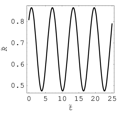
In Fig. 2, we depict $P(\tilde{R})$ and $Q(\tilde{R})/\nu^{2}$ as functions of $\tilde{R}$. The range of $\tilde{R}$ is given by $0.22\leq\tilde{R}\leq 0.75$ by solving Eq. (23) numerically, corresponding to $-1<X<1$ in Eq. (21). Here, we have taken the initial conditions as $P(\tilde{R}=0.22)=1.0$ and $dP(\tilde{R}=0.22)/(d\tilde{R})=0$ so that at a smaller curvature, $F(R)/\left(2\kappa^{2}\right)$ could contain the term $R/\left(2\kappa^{2}\right)$, i.e., the ordinary Einstein-Hilbert action. By using Eq. (25), we show the behavior of $F(\tilde{R})/\left(2\kappa^{2}\right)$ in Fig. 3. We note that the qualitative behavior of $F(\tilde{R})/\left(2\kappa^{2}\right)$ in Fig. 3 does not depend on the initial conditions and that the quantitative values of $F(\tilde{R})/\left(2\kappa^{2}\right)$ do not also depend on the initial conditions strongly. Furthermore, we illustrate $w_{\mathrm{eff}}(\tilde{R})=-1-\left[2/\left(3\beta\right)\right]X(\tilde{R})/\left(\alpha-\sqrt{1-X^{2}(\tilde{R})}\right)^{2}$ in Fig. 4. The time evolution of $\tilde{R}$ is given in Fig. 5. From Figs. 4 and 5, we see that multiple crossings of the phantom divide can be realized. We note that the results in the all figures are shown by dimensionless quantities. We also note that the lower sign in Eq. (21) leads to $0.59\leq\tilde{R}\leq 1.11$ with the results being qualitatively the same as those obtained by the upper sign above.

From Fig. 3, we see that $F(\tilde{R})$ increases in terms of $\tilde{R}$ around the present curvature $\tilde{R}(t=t_{\mathrm{p}})=12\left[2/\left(3\pi\right)\right]^{2}=0.54$. This behavior is reasonable because in the Hu-Sawicki model [22] of $F(R)$ gravity, which passes the solar system tests, $F(R)$ increases around the present curvature. We mention that such a behavior is typical for a general class of viable $F(R)$ gravities introduced in Ref. [23] to which the Hu-Sawicki model belongs. This class of modified gravities can satisfy the solar system tests and unify inflation with the late-time cosmic acceleration. As viable models of $F(R)$ gravity, e.g., the models in Refs. [24, 25, 26, 27, 28, 29] are also known (see also [30]). We remark that it is impossible to state anything on whether the reconstructed $F(R)$ gravity can pass the solar system tests and cosmological constraints at early times because the reconstructed $F(R)$ gravity cannot describe the behavior of $F(R)$ gravity for large values of $R$.

We note the stability for the obtained solutions of the phantom crossing under a quantum correction coming from the conformal anomaly. In Ref. [13], it has been shown that the quantum correction of massless conformally-invariant fields could be small when the phantom crossing occurs and therefore the solutions of the phantom crossing could be stable under the quantum correction, although the quantum correction becomes important near the Big Rip singularity. In the present model of $F(R)$ gravity with realizing multiple crossings of the phantom divide, the obtained solution can be stable because the phantom phases are transient and there is no Big Rip singularity.

Finally, we would like to remark that for the other possible solution of $\sin\nu t=+\sqrt{1-X^{2}}$, i.e., the case of the upper signs in Eqs. (23) and (24), $F(\tilde{R})$ approaches minus infinity as the curvature becomes larger than the present one although it increases in terms of $\tilde{R}$ at smaller curvature than the present one. Such a behavior is incompatible with the Hu-Sawicki model, in which $F(R)\sim R+const.$ at a much larger curvature than the present one.

In summary, we have studied the oscillating effective EoS of the universe around the phantom divide in $F(R)$ gravity. In particular, we have analyzed the behavior of $F(R)$ gravity with realizing multiple crossings of the phantom divide. Our result can be interpreted as an explicit example to illustrate that multiple phantom crossings can occur in $F(R)$ gravity as the scalar field theories such as an oscillating quintom model [16] in the framework of general relativity.

We thank Professor Sergei D. Odintsov and Professor Shin’ichi Nojiri for their collaboration in our previous work [13] and important comments. We are also grateful to Dr. Tsutomu Kobayashi for useful communications. K.B. acknowledges the KEK theory exchange program for physicists in Taiwan and the very kind hospitality of KEK. This work is supported in part by the National Science Council of R.O.C. under: Grant #s: NSC-95-2112-M-007-059-MY3 and National Tsing Hua University under Grant #: 97N2309F1 (NTHU).

References

- [1] D. N. Spergel et al. [WMAP Collaboration], Astrophys. J. Suppl. 148, 175 (2003); H. V. Peiris et al. [WMAP Collaboration], ibid. 148, 213 (2003); D. N. Spergel et al. [WMAP Collaboration], ibid. 170, 377 (2007); E. Komatsu et al. [WMAP Collaboration], ibid. 180, 330 (2009).
- [2] S. Perlmutter et al. [SNCP Collaboration], Astrophys. J. 517, 565 (1999); A. G. Riess et al. [SNST Collaboration], Astron. J. 116, 1009 (1998); P. Astier et al. [SNLS Collaboration], Astron. Astrophys. 447, 31 (2006); A. G. Riess et al., Astrophys. J. 659, 98 (2007).
- [3] P. J. E. Peebles and B. Ratra, Rev. Mod. Phys. 75, 559 (2003); V. Sahni, AIP Conf. Proc. 782, 166 (2005) [J. Phys. Conf. Ser. 31, 115 (2006)]; T. Padmanabhan, Phys. Rept. 380, 235 (2003).
- [4] E. J. Copeland, M. Sami and S. Tsujikawa, Int. J. Mod. Phys. D 15, 1753 (2006).
- [5] R. Durrer and R. Maartens, Gen. Rel. Grav. 40, 301 (2008); arXiv:0811.4132 [astro-ph].
- [6] S. Nojiri and S. D. Odintsov, eConf C0602061, 06 (2006) [Int. J. Geom. Meth. Mod. Phys. 4, 115 (2007)] [arXiv:hep-th/0601213].
- [7] S. Nojiri and S. D. Odintsov, arXiv:0801.4843 [astro-ph]; arXiv:0807.0685 [hep-th]; T. P. Sotiriou and V. Faraoni, arXiv:0805.1726 [gr-qc]; F. S. N. Lobo, arXiv:0807.1640 [gr-qc].
- [8] U. Alam, V. Sahni and A. A. Starobinsky, JCAP 0406, 008 (2004); 0702, 011 (2007); S. Nesseris and L. Perivolaropoulos, ibid. 0701, 018 (2007); P. U. Wu and H. W. Yu, Phys. Lett. B 643, 315 (2006); H. K. Jassal, J. S. Bagla and T. Padmanabhan, arXiv:astro-ph/0601389.
- [9] R. R. Caldwell, Phys. Lett. B 545, 23 (2002); S. Nojiri and S. D. Odintsov, ibid. 562, 147 (2003).
- [10] L. Amendola and S. Tsujikawa, Phys. Lett. B 660, 125 (2008).
- [11] M. C. B. Abdalla, S. Nojiri and S. D. Odintsov, Class. Quant. Grav. 22, L35 (2005).
- [12] I. H. Brevik, Int. J. Mod. Phys. D 15, 767 (2006); Gen. Rel. Grav. 38, 1317 (2006).
- [13] K. Bamba, C. Q. Geng, S. Nojiri and S. D. Odintsov, Phys. Rev. D 79, 083014 (2009).
- [14] K. Bamba and C. Q. Geng, Phys. Lett. B 679, 282 (2009).
- [15] B. McInnes, JHEP 0208, 029 (2002); R. R. Caldwell, M. Kamionkowski and N. N. Weinberg, Phys. Rev. Lett. 91, 071301 (2003).
- [16] B. Feng, M. Li, Y. S. Piao and X. Zhang, Phys. Lett. B 634, 101 (2006).
- [17] X. F. Zhang, H. Li, Y. S. Piao and X. M. Zhang, Mod. Phys. Lett. A 21, 231 (2006).
- [18] S. Nojiri and S. D. Odintsov, Phys. Rev. D 74, 086005 (2006); J. Phys. Conf. Ser. 66, 012005 (2007); J. Phys. A 40, 6725 (2007).
- [19] S. Nojiri and S. D. Odintsov, Gen. Rel. Grav. 38, 1285 (2006); Phys. Lett. B 637, 139 (2006).
- [20] E. W. Kolb and M. S. Turner, The Early Universe (Addison-Wesley, Redwood City, California, 1990).
- [21] W. L. Freedman et al. [HST Collaboration], Astrophys. J. 553, 47 (2001).
- [22] W. Hu and I. Sawicki, Phys. Rev. D 76, 064004 (2007).
- [23] G. Cognola, E. Elizalde, S. Nojiri, S. D. Odintsov, L. Sebastiani and S. Zerbini, Phys. Rev. D 77, 046009 (2008).
- [24] A. A. Starobinsky, JETP Lett. 86, 157 (2007).
- [25] S. A. Appleby and R. A. Battye, Phys. Lett. B 654, 7 (2007).
- [26] L. Amendola, R. Gannouji, D. Polarski and S. Tsujikawa, Phys. Rev. D 75, 083504 (2007).
- [27] B. Li and J. D. Barrow, Phys. Rev. D 75, 084010 (2007).
- [28] S. Tsujikawa, Phys. Rev. D 77, 023507 (2008).
- [29] S. Capozziello and S. Tsujikawa, Phys. Rev. D 77, 107501 (2008).
- [30] V. Miranda, S. E. Joras, I. Waga and M. Quartin, Phys. Rev. Lett. 102, 221101 (2009).