arXiv: 0909.1219 [hep-ph] Flavor Composition of UHE Neutrinos at Source and at Neutrino Telescopes
Abstract
We parameterize the initial flux composition of high energy astrophysical neutrinos as , where characterizes the source. All usually assumed neutrino sources appear as limits of this simple parametrization. We investigate how precise neutrino telescopes can pin down the value of . We furthermore show that there is a neutrino mixing scenario in which the ratio of muon neutrinos to the other neutrinos takes a constant value regardless of the initial flux composition. This occurs when the muon neutrino survival probability takes its minimal allowed value. The phenomenological consequences of this very predictive neutrino mixing scenario are given.
1 Introduction
Neutrino mass and mixing influences many phenomenological aspects of particle and astroparticle physics. In particular, any observed flavor mix of neutrinos and is usually not the original flavor mix, but rather a modified one. This is a consequence of the non-trivial structure of the leptonic mixing, or the Pontecorvo-Maki-Nakagawa-Saki (PMNS) mixing matrix. In this letter we wish to focus on the interplay of neutrino mixing and the flavor composition of ultra high energy (UHE) astrophysical neutrinos, whose detection is the goal of neutrino telescopes such as IceCube [1], currently under construction, or the planned KM3Net facility [2]. Many recent works discussed aspects of this problem [3, 4, 5, 6, 7, 8, 9, 10, 11, 12, 13, 14, 15, 16, 17, 18, 19, 20, 21], an overview can be found in [22].
The composition of the flux detectable in neutrino telescopes depends on two things – (i) the initial flavor composition at the source, and (ii) the standard (and possibly non-standard) parameters of neutrino mixing. This means that there are two types of studies one may pursue with neutrino telescopes:
- (a)
Neutrino physics: the extraction of neutrino properties from measurements of flavor ratios;
- (b)
Astrophysics: the identification of the initial flavor composition of the flux of UHE neutrinos and using that to probe the type of source and its properties.
A large plethora of literature exists for item (a), where authors have studied the potential of probing the neutrino mixing angles using the flavor ratios. In this paper we will concentrate on item (b) and expound the potential of UHE neutrino measurements to decipher the flavor composition of the UHE neutrinos at their source (see Ref. [20] for related recent analyses). This could lead to a better understanding of the properties of the astrophysical source responsible for the production of these neutrinos. As will be discussed in detail in Section 3, different astrophysical situations could give rise to a variety of flavor ratios of the neutrinos. Since the usually assumed high energy neutrino sources do not generate tau neutrinos in any appreciable amounts, we neglect their presence in the initial UHE neutrino flux and propose a simple one parameter parameterization of the initial flux composition of the neutrinos:
| (1) |
All discussed sources such as pion, muon-damped, charm or neutron beams are simple limits of this parameterization. With such a parameterization the experimental determination of the initial flux composition is simply an extraction of the parameter from the observed flux composition on Earth. We will define two kinds of measurable flux ratios and calculate the predicted values of these ratios at Earth for all values of from , a range which covers all possible UHE neutrino flux sources. We show that the uncertainty on the predicted values of these flux ratios due to their dependence on the oscillation parameters threatens to wash out any sensitivity of the neutrino telescopes to . We define a very simple function and show quantitatively the ranges of which could be ruled out by the data from UHE observations.
We also point out, for the first time, a special mixing scenario
for which the
observable ratio of muon neutrinos to the other neutrinos is
independent of the initial mixing scenario. This occurs when the
averaged survival probability for muon neutrinos takes its minimal
allowed value of .
It illustrates
nicely that the ratio of muon neutrinos with the other flavors alone
may not be a good discriminator of different sources.
Our paper is build up as follows: in Section 2 we summarize the neutrino mixing phenomenology framework at neutrino telescopes. Section 3 sees the discussion of several neutrino sources whose common features lead to the parameterization in Eq. (1). The peculiar mixing scenario with a constant muon neutrino flux with respect to the total flux is presented in Section 4. The experimental determination of is investigated in Section 5, before we sum up and conclude in Section 6.
2 Neutrino Mixing and Neutrino Telescopes
Astrophysical sources will generate fluxes of electron, muon and tau neutrinos, denoted by , and , respectively. As a consequence of non-trivial neutrino mixing, it is not this initial flux composition which arrives at terrestrial detectors. In fact, what is measurable is given by11 1 Everywhere in this paper we denote the fluxes at the source with a superscript 0 (), while the observed fluxes will be denoted without any superscript.
| (2) |
where the neutrino mixing probability is
| (3) |
and is the lepton mixing matrix. The current best-fit values as well as the allowed , and ranges of the oscillation parameters are [23]
| (4) |
These mixing angles can be related to elements of the PMNS mixing matrix via
| (5) |
where , . The CP phase is unknown. Because the travelled distance of the neutrinos is much larger than the oscillation length , the mass-squared differences drop out of the mixing probabilities. Furthermore, solar neutrino mixing is neither maximal, nor zero or , and due to these reasons no transition probability with is zero and no survival probability is one [11]. Consequently, high energy astrophysical neutrinos will always mix. To be precise, at and the entries of the flavor conversion matrix are
| (6) |
The consequences and phenomenology of the special values and will be dealt with in Section 4.
As is obvious from the ranges of the mixing parameters given above, a good zeroth order description of neutrino mixing is
| (7) |
Therefore, it proves in particular useful to expand in terms of
| (8) |
Note that . The result of the expansion for the flavor mixing matrix is
| (9) |
where the universal first [8, 11] and second [17, 18] order correction terms are
| (10) |
We have also given the expressions for the value . Note that is positive semi-definite. The same holds for the third expansion parameter
| (11) |
which is usually only a sub-leading correction. The parameter can seldomly be larger than the first order term . To be quantitative,
| (12) |
The dependence of the expansion parameters on is weak. From the expressions for and it is clear that their dependence on the atmospheric neutrino mixing angle is stronger than the one on [19].
3 Initial Flux Compositions and their Parametrization
We now turn to the observable flavor ratios [24, 25]. The most frequently considered and experimentally most accessible is the ratio of flux of muon neutrinos to that of all other flavors:
| (13) |
Often one considers also the ratio , which is simply . Whereas muon neutrinos with their characteristic tracks (continuous loss of energy via Cerenkov radiation) can be somewhat easily distinguished from electron and tau neutrinos, the distinction of the latter two is more difficult. If possible (e.g., via electromagnetic vs. hadronic showers, or tau-induced lollipop/double bang events), one may consider their ratio as well:
| (14) |
We will use these ratios and in this paper. When neutrinos and anti-neutrinos are not distinguished, then two independent ratios are sufficient to fully determine the flavor content. For instance, if both and are known, the ratio of muon neutrinos to tau neutrinos is related to and via .
In what regards initial flux compositions, typically one considers pionic beam-dump-like sources, which have an initial flux composition of
| (15) |
They arise because hadronic processes in a cosmic ray source produce pions. If the medium in such a source is opaque to muons, then one speaks of muon-damped cases [26], which have a composition of:
| (16) |
Another possibility are so-called neutron beams, which result when photo-disintegration creates neutrons from nuclei [27], and therefore
| (17) |
Finally, at high energies semileptonic decays of charm quarks22 2 For bottom quark decays the production rate is suppressed by one order of magnitude. may generate an initial flavor ratio of [28]
| (18) |
We see that in all sources no tau neutrinos are generated initially. There is in fact always a small component (“prompt ”) from decays such as , however this contribution is at most at the permille level and can safely be neglected. We stress however that all of the above sources can be expected to be “impure”, i.e., there will be small deviations from the idealized compositions given above [13, 9, 18]. As one example, Ref. [13] has argued that because of the wrong helicity polarization of the muons in pion decay the have actually a softer spectrum, and thus the effective count of muon neutrinos is reduced. This depends on the injection spectrum, which is described by the power law . For the canonical value it was found that effectively . It was shown [18] that inclusion of leptonic and semi-leptonic kaon decays, as well as of heavy flavor decays does not change this ratio appreciably.
One may also consider GZK-neutrinos [29], whose flavor content
changes with energy. Below about 100 PeV ( GeV) one has
, whereas for higher energies .
Given all the above discussion, we are lead to parameterize the initial flux composition of high energy neutrinos simply as
| (19) |
The experimental determination of the initial flux composition is therefore simply an extraction of the parameter from the observed flux composition on Earth33 3 Ref. [6] has proposed .. From Eq. (19) one can obtain (pure) pion sources when , neutron beams for , charm sources for and muon-damped sources when one takes the limit .
Let us attempt to express the flux ratios and in a source-independent way. We take advantage of the parametrization in Eq. (19) and use the expansion of the probabilities in Eq. (9). First we consider the ratio of muon to all neutrinos and find
| (20) |
| pion | 2 | ||||
| charm | 1 | ||||
| neutron | 0 | ||||
| muon-damped | |||||
We note the following points from this expression:
- •
for , which corresponds to pionic sources, there is no explicit dependence on and also corrections due to vanish. The uncertainty on is hence expected to be amongst the lowest for this case;
- •
for , which corresponds to charm sources, there is no first order correction , and thus corrections to the zeroth order expression are only of quadratic order in the small expansion parameters and ;
In the zeroth order approximation, which corresponds to – symmetry yielding and such that the correction terms , and are all vanishing, Eq. (20) reduces to
where we have also given the simple expressions for the special values of corresponding to the usual sources one considers. Hence, we note that all sources have similar predicted around 0.3. Indeed, in Section 4 we will present an extreme scenario in which independent of . We further note that the predicted is highest for , lowest for and intermediate for and 2. In general, slightly increases with .
Similarly, the ratio of electron and tau neutrinos is
| (21) |
Here the value removes again several correction terms, in particular the terms with explicit dependence on , which leads to small uncertainty. For the case of – symmetry one finds
The spread for the different values of is larger than for . For instance, if then at leading order and between for the range, while leads to at leading order and between for the range. In general, slightly decreases with .
In Fig. 1 we show and as a function of . In Table 1 we present the 1 and 3 ranges of predicted and for the 4 benchmark cases of corresponding to pion, charm, neutron and muon-damped sources. The 1 and 3 ranges of and correspond to current 1 and ranges of the oscillation parameters. In general one notes again that is not an ideal discriminator in order to distinguish the neutrino source, because it is rather close to for all . Therefore, at the present stage we can already suspect that the task of identifying will be easier when is added to the statistics. A more detailed analysis will be presented in Section 5.


4 An Extreme Case: Minimal Survival Probabilities
One observes from the allowed ranges of the oscillation probabilities in Eq. (6) that and can take the value when the ranges of the oscillation parameters are inserted. It is worth noting that is the minimal value that an averaged survival probability can take if there are 3 fermion families. In general, in the presence of flavors we have
| (22) |
The minimum is obtained if and only if for all , i.e., when all mixing matrix elements of a row take on the same value44 4 Note that this concerns the elements of a row. Commonly it is assumed the elements of a column are identical (as for tri-bimaximal, or more general tri-maximal mixing [30])..
Considering the case of , let us discuss first the phenomenological consequences of . The case of will be discussed at the end of this Section. First we note that unitarity of the PMNS matrix links the three entries of a row, which implies that only two independent constraints can result. The first one stems from and is
| (23) |
Inserting this in gives the second independent constraint
| (24) |
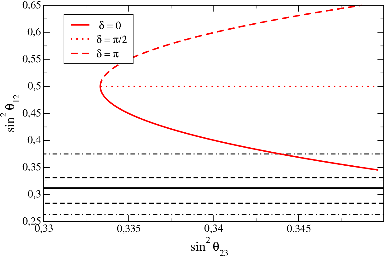
We immediately see that should be rather large, significantly less than and should be different from zero, or different from 1. We display the phenomenology resulting from Eqs. (23, 24) in Fig. 2. While lies close to its lower bound, can approach its upper bound from above, in which case is close to its current upper bound and less than one (or larger than 5). Vanishing leads to maximal and is disallowed.
The condition together with unitarity of the PMNS matrix fix the form of the matrix , namely
| (25) |
Recall that the , and therefore the averaged probabilities , depend on four independent parameters. The condition fixes two of the four parameters and we have chosen and as the remaining two free and independent parameters. It is easy to see that from Eq. (25) the relation
| (26) |
follows. With this relation one obtains a remarkably simple result for the ratio as a function of , namely
| (27) |
regardless of !
The origin of this simple result is of course that all
neutrinos have an equal share in , i.e., their
muon content is equally distributed55
5
Similarly, the ratio of
muon neutrinos to the sum of electron and tau neutrinos is
..
Concerning , the general result as a function of is
rather lengthy. The allowed ranges of are however
significantly less than for the unconstrained case.
For instance, for pion sources lies
between 1.23 and 1.40, to be compared with the general
allowed range between 0.82 and 1.45. An interesting case occurs for
muon-damped sources, for which we find that .


If the third row of has identical entries, and therefore , then
| (28) |
and
| (29) |
While the second constraint is very similar to the one for , the first condition implies here that lies slightly outside its allowed range. The value found in Eq. (6) is therefore only numerically close to . In any case, since the identification of muon neutrinos is much simpler than of tau neutrinos, it makes little sense to discuss the scenario with a saturated .
5 Experimental Distinction of Sources

In this Section we explore the potential of the neutrino telescopes to ascertain the initial flux composition at the source. We stress that all results to be shown have been obtained by an exact calculation of the oscillation probabilities. We begin by returning to Fig. 1, in which we display the current predicted ranges of and respectively, as a function of the flux composition parameter . For each value of we calculated the full range of predicted values of and by allowing the oscillation parameters to vary in their current allowed range [23]. The range of values of and for the different limiting cases are given in Table 1. As discussed before, we note from the figure that the ranges for all are overlapping. We also note that the spread in is minimized for values of close to 2, as for this case the explicit dependence on vanishes (cf. Eq. (20)). For the same reason, the spread in is also minimized for values of close to 2 (cf. Eq. (21)). The spread in for small is somewhat larger than for large . The spread in for small is seen to be significantly larger than for large . The large spread for small of both and implies that neutron sources have the largest dependence on the neutrino mixing parameters. Note that while the possible spread induced by neutrino mixing is smallest for between 1 and 2, it does not necessarily imply that the sensitivity to initial flux composition will be best for these cases. We also note that appears to be a much better discriminator for compared to and hence inclusion of in addition to will make the identification of the source easier. The individual lines embedded in the band in Fig. 1 show the predicted and for several benchmark mixing scenarios, in which the values of the oscillation parameters are
- “TBM”
the tri-bimaximal scenario: the oscillation parameters are , , and ;
- “EX1”
extreme scenario 1: the oscillation parameters are , , and ;
- “EX2”
extreme scenario 2: the oscillation parameters are , , and ;
- “SPL”
special scenario: for the special scenario discussed in the previous Section, we take , , and .
One can immediately see from Fig. 1 that as predicted in Section 4, the special case yields for all values of . Therefore, if this case was the true mixing scenario chosen by Nature, then it would be impossible to conclude anything about from measurement at neutrino telescopes. One can also note that for the EX1 mixing case is very close to the SPL case and hence it would also be difficult to say anything about the source, if this set of mixing parameters turn out to be the true mixing angles.

We next define a very simple function as66 6 We are aware that this definition of is not strictly valid for a ratio as its error will not be Gaussian. Nonetheless we use it here for the sake of simplicity as the purpose of this paper is to roughly illustrate the potential of the neutrino telescope rather than to show exact numerical results for which one should work with the actual number of events calculated using a detailed code for the detector including threshold, efficiencies and so on.
| (30) |
where can be either or and “”
and “” refer to
observed and predicted flux ratios respectively, and
is the 1 experimental error on the
relevant flux ratio. We show results for fixed experimental errors
of 20%, 10% and 5% for and 30%, 20% and 10% for .
We generate the “” at certain “true” values , denoted as
, and at one of the
benchmark mixing scenarios given above. This
is then fitted with corresponding to .
The oscillation parameters in the fit are generally allowed to
vary freely in the fit, apart from Fig. 3.
In Fig. 3 we show the obtained
as a function of for and TBM mixing.
All oscillation parameters are kept fixed at their TBM values
in the fit for this figure.
We reiterate that
is defined
as the value of for which the
() are generated
and is the value of in ().
The best-fit comes at , as expected. We can see that
extremely good sensitivity to comes for , while
reasonable sensitivity to is expected if .
For one finds hardly any sensitivity at all,
even in this ideal case, where the effect of oscillation
parameter uncertainties have been neglected. If could be
measured at the neutrino telescope, then we expect
good sensitivity even if .


Now we allow the
oscillation parameters to vary freely in the fit –
the only restriction being that they are not allowed to take
values beyond their current limits.
We find that, as expected from Fig. 1,
there is absolutely no sensitivity if is used.
The reason, as discussed before,
is the following: for TBM mixing parameters for
. This
value of can be reproduced by all values of , as long
as we are allowed to pick the most suitable set of
oscillation parameters which lie within the current limit.
Therefore, for this case the always exactly reproduces
the and thus for all . For
the situation is slightly better. for
TBM mixing and . And hence, as predicted from
Fig. 1, values of can still
be disfavored. The reason being that for , it
is impossible to get the close to 1.
However, for , one can always find
a set of oscillation parameters within the still allowed region
which gives the same .
Fig. 4 shows the result of the fit.


So far we have shown all sensitivity results assuming
that we had . We next show contour plots
in the plane in Figs. 5 and
6. The way these figures are to be interpreted
is the following: for each on the -axis,
the shaded region shows the values of
which can be excluded at .
Fig. 5
shows the sensitivity on of the neutrino telescope using
the more powerful flavor ratio , while Fig. 6
gives the corresponding reach by using the more easily
measurable . The darkest (black) regions are
obtained assuming that we have 10% (5%) uncertainty in
(), the dark (green) regions are for an uncertainty
of 20% (10%) in (), while the lightest (cyan) regions
are for uncertainty of 10% (5%) in ().
We show these regions in Fig. 5
for the four benchmark sets
of mixing parameter cases that we have considered in this paper.
The upper left hand panel is for TBM mixing, the upper right hand
panel is for the “EX1” oscillation scenario, the lower
left hand panel is for the “EX2” oscillation case and the
lower right hand for the special case (“SPL”)
of trimaximal mixing in the
second row. For we show the cases for “TBM” and “EX2”
only in Fig. 6.
The way we have generated these figures is the following:
for each value of we generate the data for the particular
oscillation parameter set. For instance for the upper left hand
panel of Fig. 5
the data is always generated for the TBM mixing parameters.
This data is then fitted with any value of ,
while all oscillation parameters are allowed to vary
within their allowed
range. From Fig. 5 we
find that the neutrino telescopes have reasonable
sensitivity to the initial flux composition if can be
measured with reasonable precision. The sensitivity
depends sharply on the true value of the oscillation parameters
as well as on the true value of . We also note that irrespective
of the true oscillation parameter scenario, there is a narrow
band around , where we have no sensitivity to the
initial flux composition.
From Fig. 6 we see
that for TBM mixing and
EX2, returns a sensitivity which is not bad. In particular,
for TBM mixing, which is the currently favored scenario,
one finds reasonable sensitivity to the flux composition
if . On the other hand we have
numerically checked that if the true neutrino
mixing turns out to be compatible with the EX1 and SPL case,
then it would be almost impossible to determine the
UHE neutrino initial flavor composition using alone.
In other words, there are no shaded regions for
SPL and EX1 in the space. This is why
we do not show the panels for these cases in Fig. 6.
Of course it is expected that the current uncertainties on the oscillation parameters will decrease [31], as better neutrino oscillation experiments are built and more data is accumulated. This would improve further the prospects of measuring at neutrino telescopes.
6 Conclusions and Summary
Observation of neutrinos with very high energies coming from astrophysical sources has been long overdue. The observed UHE fluxes have a flavor composition on Earth which depends on both their initial composition at source as well as on neutrino flavor oscillations. Therefore, it should be possible to study both kinds of physics with these observations – neutrino physics as well as physics concerning the UHE neutrino sources. Unfortunately, since there are uncertainties in both neutrino mixing parameters as well as knowledge on the type of sources of these UHE neutrinos, attempts on determining one are always plagued by uncertainties on the other.
In this paper we attempted to probe the potential of the future neutrino telescopes in deciphering the flavor composition of the UHE neutrino flux at source. We did this by proposing a very simple and minimal parametrization of the flavor composition at source. We parameterized the initial flux composition of high energy neutrinos simply as
| (31) |
The parameter can take any value from to . Specific values of describe the pure known sources. The UHE neutrino flux depends on a number of astrophysical factors and its exact flavor composition will depend on the process which generates this flux. Neutrinos coming from pion decay will have a flavor ratio of . Likewise a muon-damped source will give a ratio of , a neutron beam source will give and a charm source . One expects impurities in these relations, i.e., they will not be in the exact form given above. The astrophysical source producing the UHE neutrinos could have a combination of some or all such processes producing these neutrinos. Also, unless there are close-by astrophysical sources, what will be detected at the neutrino telescope is most likely going to be a diffuse flux coming from a combination of different astrophysical sources, and hence it is expected that this observed flux would come as a combination of different neutrino generating decay processes. Since the number of produced at the source is negligible, our one parameter description is the most economical and general way of probing the initial flavor composition of the UHE neutrinos.
The observed flavor ratios depend on the neutrino mixing parameters
in addition to the property of the source.
We studied two of the most used observed flux
ratios and
.
We wrote down approximate analytic forms for these flux
ratios in terms of and the mixing parameters. Using exact
numerical results
we showed the uncertainty in and coming from the
current uncertainty on the mixing parameters. It was shown that the
uncertainties due to mixing parameters in minimum around
.
We also showed that for both and the uncertainty due to
mixing for small was more than that for large . We also
pointed out a special case where for all values of .
This scenario corresponds to the case where the second row of the
neutrino mixing matrix has equal entries in all its three elements and
illustrates that the ratio alone may not suffice to probe .
We next defined a simple function and expounded the
potential of the neutrino telescopes in determining and
hence the UHE neutrino flux composition at source.
Since the forthcoming neutrino telescopes are yet to collect
any data on ultra high energy neutrino
fluxes, and since it is not yet known
what kind of total uncertainty we would have on the observed
flux ratios,
we performed the analysis for four benchmark points in the
mixing parameter space and by assuming different values of
errors on and .
Those errors cover assumptions ranging from plausible to
optimistic, and allow to compare the prospects of
neutrino telescopes.
In particular, our analysis shows what kind of
statistics and systematics are required from neutrino telescopes
in order to achieve UHE source flavor sensitivity.
We first studied the case by
assuming a pure pionic source. It was seen that in this case,
once the uncertainties
due to oscillation parameters were taken into account,
as measured in neutrino telescopes could
give absolutely no information about the flux composition at source.
The measured could still be used to exclude certain
ranges of
and hence certain types of sources. Finally, we performed a full
scan of the space, where data was generated at every value of
and the potential of the data to pick the right source
was studied. We presented contours
in the
parameter space, which give the initial
flux composition sensitivity of the
neutrino telescope, as a function of .
In conclusion, neutrino telescopes will provide information on the flavor composition of the UHE neutrino fluxes on Earth. This can be used to study the initial flavor composition of these fluxes at their source. Reasonable sensitivity to deciphering the correct source flavor composition is expected from these experiments, despite the current uncertainties on the mixing parameters. With projected improvements in our understanding of the neutrino mixing angles, the source flavor sensitivity of the neutrino telescopes will improve.
Acknowledgments
We thank Sergio Palomares-Ruiz for helpful comments. W.R. was supported by the ERC under the Starting Grant MANITOP and by the Deutsche Forschungsgemeinschaft in the Sonderforschungsbereich Transregio 27 “Neutrinos and beyond – Weakly interacting particles in Physics, Astrophysics and Cosmology”. S.C. wishes to thank the Max–Planck–Institut für Kernphysik, Heidelberg, where part of this work was completed and acknowledges support from the Neutrino Project under the XI Plan of Harish–Chandra Research Institute.
References
- [1] J. Ahrens et al. [The IceCube Collaboration], Nucl. Phys. Proc. Suppl. 118, 388 (2003) [astro-ph/0209556].
- [2] Information available at http://www.km3net.org
- [3] S. Pakvasa, Mod. Phys. Lett. A 19, 1163 (2004) [Yad. Fiz. 67, 1179 (2004)] [arXiv:hep-ph/0405179].
- [4] P. Bhattacharjee and N. Gupta, arXiv:hep-ph/0501191.
- [5] P. D. Serpico and M. Kachelriess, Phys. Rev. Lett. 94, 211102 (2005) [arXiv:hep-ph/0502088]; P. D. Serpico, Phys. Rev. D 73, 047301 (2006) [arXiv:hep-ph/0511313].
- [6] Z. Z. Xing and S. Zhou, Phys. Rev. D 74, 013010 (2006) [arXiv:astro-ph/0603781].
- [7] W. Winter, Phys. Rev. D 74, 033015 (2006) [arXiv:hep-ph/0604191].
- [8] Z. Z. Xing, Phys. Rev. D 74, 013009 (2006) [arXiv:hep-ph/0605219].
- [9] M. Kachelriess and R. Tomas, Phys. Rev. D 74, 063009 (2006) [arXiv:astro-ph/0606406]; M. Kachelriess, S. Ostapchenko and R. Tomas, Phys. Rev. D 77, 023007 (2008) [arXiv:0708.3047 [astro-ph]].
- [10] D. Majumdar and A. Ghosal, Phys. Rev. D 75, 113004 (2007) [arXiv:hep-ph/0608334].
- [11] W. Rodejohann, JCAP 0701, 029 (2007) [arXiv:hep-ph/0612047].
- [12] D. Meloni and T. Ohlsson, Phys. Rev. D 75, 125017 (2007) [arXiv:hep-ph/0612279].
- [13] P. Lipari, M. Lusignoli and D. Meloni, Phys. Rev. D 75, 123005 (2007) [arXiv:0704.0718 [astro-ph]].
- [14] R. L. Awasthi and S. Choubey, Phys. Rev. D 76, 113002 (2007) [arXiv:0706.0399 [hep-ph]].
- [15] K. Blum, Y. Nir and E. Waxman, arXiv:0706.2070 [hep-ph].
- [16] G. R. Hwang and K. Siyeon, Phys. Rev. D 78, 093008 (2008) [arXiv:0711.3122 [hep-ph]].
- [17] S. Pakvasa, W. Rodejohann and T. J. Weiler, Phys. Rev. Lett. 100, 111801 (2008) [arXiv:0711.0052 [hep-ph]]
- [18] S. Pakvasa, W. Rodejohann and T. J. Weiler, JHEP 0802, 005 (2008) [arXiv:0711.4517 [hep-ph]].
- [19] S. Choubey, V. Niro and W. Rodejohann, Phys. Rev. D 77, 113006 (2008) [arXiv:0803.0423 [hep-ph]].
- [20] A. Esmaili and Y. Farzan, Nucl. Phys. B 821, 197 (2009) [arXiv:0905.0259 [hep-ph]]; see also K. C. Lai, G. L. Lin and T. C. Liu, arXiv:0905.4003 [hep-ph].
- [21] J. F. Beacom, N. F. Bell, D. Hooper, S. Pakvasa and T. J. Weiler, Phys. Rev. Lett. 90, 181301 (2003) [arXiv:hep-ph/0211305]; Phys. Rev. D 69, 017303 (2004) [arXiv:hep-ph/0309267]; P. Keranen, J. Maalampi and J. T. Peltoniemi, Phys. Lett. B 461, 230 (1999) [arXiv:hep-ph/9901403]; K. Enqvist, P. Keranen and J. Maalampi, Phys. Lett. B 438, 295 (1998) [arXiv:hep-ph/9806392]; H. Minakata and A. Y. Smirnov, Phys. Rev. D 54, 3698 (1996) [arXiv:hep-ph/9601311]; D. Hooper, D. Morgan and E. Winstanley, Phys. Lett. B 609, 206 (2005) [arXiv:hep-ph/0410094]; J. F. Beacom, N. F. Bell, D. Hooper, J. G. Learned, S. Pakvasa and T. J. Weiler, Phys. Rev. Lett. 92, 011101 (2004) [arXiv:hep-ph/0307151]; P. Keranen, J. Maalampi, M. Myyrylainen and J. Riittinen, Phys. Lett. B 574, 162 (2003) [arXiv:hep-ph/0307041]; S. Goswami and W. Rodejohann, JHEP 0710, 073 (2007) [arXiv:0706.1462 [hep-ph]]; M. Maltoni and W. Winter, JHEP 0807, 064 (2008) [arXiv:0803.2050 [hep-ph]]; M. Blennow and D. Meloni, arXiv:0901.2110 [hep-ph].
- [22] S. Pakvasa, Mod. Phys. Lett. A 23, 1313 (2008) [arXiv:0803.1701 [hep-ph]].
- [23] G. L. Fogli, E. Lisi, A. Marrone, A. Palazzo and A. M. Rotunno, Phys. Rev. Lett. 101, 141801 (2008) [arXiv:0806.2649 [hep-ph]]; M. Maltoni, T. Schwetz, M. A. Tortola and J. W. F. Valle, New J. Phys. 6, 122 (2004) [arXiv:hep-ph/0405172]; A. Bandyopadhyay, S. Choubey, S. Goswami, S. T. Petcov and D. P. Roy, arXiv:0804.4857 [hep-ph].
- [24] J. F. Beacom, N. F. Bell, D. Hooper, S. Pakvasa and T. J. Weiler, Phys. Rev. D 68, 093005 (2003) [Erratum-ibid. D 72, 019901 (2005)] [arXiv:hep-ph/0307025].
- [25] L. Anchordoqui and F. Halzen, Annals Phys. 321, 2660 (2006) [arXiv:hep-ph/0510389].
- [26] J. P. Rachen and P. Meszaros, Phys. Rev. D 58, 123005 (1998); T. Kashti and E. Waxman, Phys. Rev. Lett. 95, 181101 (2005) [arXiv:astro-ph/0507599].
- [27] L. A. Anchordoqui, H. Goldberg, F. Halzen and T. J. Weiler, Phys. Lett. B 593, 42 (2004) [arXiv:astro-ph/0311002].
- [28] R. Enberg, M. H. Reno and I. Sarcevic, Phys. Rev. D 78, 043005 (2008) [arXiv:0806.0418 [hep-ph]]; Phys. Rev. D 79, 053006 (2009) [arXiv:0808.2807 [astro-ph]]; R. Gandhi, A. Samanta and A. Watanabe, arXiv:0905.2483 [hep-ph].
- [29] V. S. Beresinsky and G. T. Zatsepin, Phys. Lett. B 28, 423 (1969); R. Engel, D. Seckel and T. Stanev, Phys. Rev. D 64, 093010 (2001) [arXiv:astro-ph/0101216].
- [30] J. D. Bjorken, P. F. Harrison and W. G. Scott, Phys. Rev. D 74, 073012 (2006) [arXiv:hep-ph/0511201]; X. G. He and A. Zee, Phys. Lett. B 645, 427 (2007) [arXiv:hep-ph/0607163]; C. S. Lam, Phys. Rev. D 74, 113004 (2006) [arXiv:hep-ph/0611017]; W. Grimus and L. Lavoura, JHEP 0809, 106 (2008) [arXiv:0809.0226 [hep-ph]]; Phys. Lett. B 671, 456 (2009) [arXiv:0810.4516 [hep-ph]]; C. H. Albright and W. Rodejohann, Eur. Phys. J. C 62, 599 (2009) [arXiv:0812.0436 [hep-ph]]; C. S. Lam, arXiv:0907.2206 [hep-ph].
- [31] A. Bandyopadhyay et al. [ISS Physics Working Group], arXiv:0710.4947 [hep-ph]; P. Huber, M. Lindner, T. Schwetz and W. Winter, arXiv:0907.1896 [hep-ph]; A. Bandyopadhyay, S. Choubey, S. Goswami and S. T. Petcov, Phys. Rev. D 72, 033013 (2005) [arXiv:hep-ph/0410283].