General physical properties of bright Fermi blazars
Abstract
We studied all blazars of known redshift detected by the Fermi satellite during its first three–months survey. For the majority of them, pointed Swift observations ensures a good multiwavelength coverage, enabling us to to reliably construct their spectral energy distributions (SED). We model the SEDs using a one–zone leptonic model and study the distributions of the derived interesting physical parameters as a function of the observed –ray luminosity. We confirm previous findings concerning the relation of the physical parameters with source luminosity which are at the origin of the blazar sequence. The SEDs allow to estimate the luminosity of the accretion disk for the majority of broad emitting line blazars, while for the line–less BL Lac objects in the sample upper limits can be derived. We find a positive correlation between the jet power and the luminosity of the accretion disk in broad line blazars. In these objects we argue that the jet must be proton–dominated, and that the total jet power is of the same order of (or slightly larger than) the disk luminosity. We discuss two alternative scenarios to explain this result.
Keywords:
BL Lacertae objects: general — quasars: general — radiation mechanisms: non–thermal — gamma-rays: theory — X-rays: general1 Introduction
The Large Area Telescope (LAT) onboard the Fermi Satellite, in the first months of operation succeeded to double the number of know –ray emitting blazars (Abdo et al. 2009a, hereafter A09). Excluding radio–galaxies, in the list of the LAT 3–months survey we have 104 blazars, divided into 58 Flat Spectrum Radio Quasars (FSRQs, including one Narrow Line Seyfert 1 galaxy), 42 BL Lacs and 4 sources of uncertain classification. Of these, 89 have a known redshift, and a large fraction of sources have been observed with the Swift satellite within the 3 months survey, while others have been observed by Swift at other epochs.
The combination of Fermi and Swift data are of crucial importance for the modelling of these blazars, even if the LAT data are an average over the 3 months of the survey, so that, strictly speaking, we cannot have a really simultaneous optical to X–ray SED, even when the Swift observations have been performed during the three months of the survey. Despite this, the optical/UV, X–ray and –ray coverage can often define or strongly constrain the position and the flux levels of both peaks of the non–thermal emission of blazars. Furthermore, as discussed in Ghisellini, Tavecchio & Ghirlanda (2009, hereafter Paper 1), the data from the UV Optical Telescope (UVOT) of Swift are often crucial to disentangle the non–thermal beamed jet emission from thermal radiation produced by the accretion disk. When the accretion disk is visible it is then possible to estimate both the mass of the black hole and the accretion luminosity and to compare it with the power carried by the jet. In Paper I we did this study for the 23 most luminous blazars, exceeding, in the –ray range, an observed luminosity of erg s-1. In Tavecchio et al. (2009, hereafter T09) we considered the BL Lac objects detected by Fermi with the aim to find, among those, the best candidates to be TeV emitters. Here we extend these previous studies to the entire Fermi blazar sample of the 3 months survey. Besides finding the intrinsic physical properties characterising the emitting region of these Fermi blazars, like magnetic field, particle density, size, beaming factor and so on, the main goal of our study is to investigate if there is a relation between the jet power and the disk luminosity, as a function of the –ray luminosity.
This implies two steps. First we collect the data to construct the SED of all sources, taking advantage of possible Swift observations, that we analyse, and of archival data taken from the NASA Extragalactic Database (NED, http://nedwww.ipac.caltech.edu/. Secondly, we apply a model to fit these data, that returns the value of the physical parameters of the emitting region, and, if possible, the value of the accretion disk luminosity and of the black hole mass. We do this for all the 85 sources (out of 89) with a minimum coverage of the SED. Among these blazars, there are several BL Lac objects for which there is no sign of thermal emission produced by a disk, nor of emission lines produced by the photo–ionising disk photons. For them we derive an upper limit of the luminosity of a standard, Shakura–Sunyaev (1973) disk. We also derive the distributions of the needed physical parameters, and their dependence on the –ray luminosity and on the presence/absence of a prominent accretion disk. As expected, the jets of line–less BL Lacs have less power than broad line FSRQs, have bluer spectra, and their emitting electrons suffer less radiative cooling. This confirms earlier results (Ghisellini et al. 1998) explaining the so called blazar sequence (Fossati et al. 1998).
The main result of our analysis concerns the relation between the jet power and the accretion disk luminosity. We find that they correlate in FSRQs, for which we can estimate both the black hole mass and the accretion luminosity. We discuss two alternative scenarios to explain this behaviour. For BL Lacs (with only an upper limit on the accretion luminosity), we suggest that the absence of any sign of thermal emission, coupled to the presence of a relatively important jet, strongly suggests a radiatively inefficient accretion regime.
In this paper we use a cosmology with and , and use the notation in cgs units (except for the black hole masses, measured in solar mass units).
2 The sample
Tab. 1 lists the 89 blazars with redshift of the A09 catalogue of Fermi detected blazars. Besides their name, we report the redshift, the K–corrected –ray luminosity in the Fermi/LAT band, (see e.g. Ghisellini, Maraschi & Tavecchio 2009), if there are observations by the Swift satellite, if the source was detected by EGRET and the classification. For the latter item we have maintained the same classification as in A09, but we have indicated those sources classified as BL Lac objects but that do have broad emission lines.
The distinction between BL Lacs and FSRQs is traditionally based on the line equivalent width (EW) being smaller or larger than 5Å. With this definition, we classify as BL Lacs those sources having genuinely very weak or absent lines and also objects with strong lines but whose non–thermal continuum is so enhanced to reduce the line EW. This second category of “BL Lacs” should physically be associated to FSRQs. We have tentatively made this distinction on Tab. 1, based on some information from the literature about the presence, in these objects, of strong broad lines. In the rest of the paper we will consider them as FSRQs.
The source PMN 0948–0022 belongs to still another class, being a Narrow Line Seyfert 1 (NLSy1; FWHM1500 km s-1). This source has been discussed in detail in Abdo et al. (2009b) and Foschini et al. (2009): its SED and general properties are indistinguishable from FSRQs and we then assign this source to this group.
We then have 57 FSRQs, 1 NLSy1 and 31 BL Lac objects. Of the latter, 6 have strong broad lines or have been also classified as FSRQs (by Jauncey et al. 1989). Four of the FSRQs (indicated with the superscript in Table 1) do not have a sufficient data coverage to allow a meaningful interpretation, and we will not discuss them. The 23 blazars (21 FSRQs and 2 BL Lacs, but with broad emission lines) with an average –ray luminosity exceeding erg s-1 written in italics have been discussed in Paper 1. The 25 underlined BL Lacs are discussed in T09. One of these, (0814+425=OJ 425) is shown also here, since it can be fitted both with a pure synchrotron self–Compton (SSC) and an “External Compton” (EC) model (see next section).
In summary, in this paper we present the SED and the corresponding models for 37 blazars: 32 FSRQs and 5 BL Lacs that are suspected to be FSRQs with broad lines hidden by the beamed continuum. However, when discussing the general properties of the Fermi blazars, we will consider the entire blazar sample of Tab. 1, with the only exception of the 4 FSRQs with a very poor data coverage. These are 85 sources. To this aim we will use the results of Paper 1, concerning the most –ray luminous blazars, and we will apply our model also to the BL Lacs shown in T09. For the ease of the reader, we report in Table 4 and Table 5 the physical parameters of all the 85 blazars.
| Name | Alias | S? | E? | Type | ||
|---|---|---|---|---|---|---|
| 0017–0512n | CGRaBS | 0.227 | 45.96 | Y | Y | Q |
| 00311–1938 | KUV | 0.610 | 46.40 | Y | B | |
| 0048–071 | PKS | 1.975 | 48.2 | Q | ||
| 0116–219 | PKS | 1.165 | 47.68 | Q | ||
| 0118–272 | PKS | 0.559 | 46.48 | UL | B | |
| 0133+47 | DA 55 | 0.859 | 47.41 | Y | UL | Q |
| 0142–278 | PKS | 1.148 | 47.63 | Q | ||
| 0202–17 | PKS | 1.74 | 48.2 | UL | Q | |
| 0208–512 | PKS | 1.003 | 47.92 | Y | Y | Q |
| 0215+015 | PKS | 1.715 | 48.16 | Y | UL | Q |
| 0218+35 | B2 | 0.944 | 47.47 | Y | UL | Q |
| 0219+428 | 3C66A | 0.444 | 47.16 | Y | Y | B |
| 0227–369 | PKS | 2.115 | 48.6 | Y | Q | |
| 0235+164 | AO | 0.94 | 48.4 | Y | Y | B∗ |
| 0301–243 | PKS | 0.260 | 45.77 | Y | UL | B |
| 0332–403 | PKS | 1.445b | 47.68 | Y | UL | B∗∗ |
| 0347–211 | PKS | 2.944 | 49.1 | Y | Q | |
| 0426–380 | PKS | 1.112 | 48.06 | Y | UL | B∗ |
| 0447–439 | PKS | 0.107 | 46.03 | Y | B | |
| 0454–234 | PKS | 1.003 | 48.16 | Y | Y | Q |
| 0502+675 | 1ES | 0.314 | 46.06 | Y | B | |
| 0528+134 | PKS | 2.04 | 48.8 | Y | Y | Q |
| 0537–441 | PKS | 0.892 | 47.99 | Y | Y | B∗ |
| 0650+453 | B3 | 0.933 | 47.82 | Y | Q | |
| 0713+1935n | CLASS | 0.534 | 46.84 | Q | ||
| 0716+332 | TXS | 0.779 | 47.12 | Y | Q | |
| 0716+714 | TXS | 0.26 | 46.55 | Y | Y | B |
| 0735+178 | PKS | 0.424 | 46.31 | Y | Y | B |
| 0814+425 | OJ 425 | 0.53 | 46.87 | Y | UL | B |
| 0820+560 | S4 | 1.417 | 48.01 | Y | Q | |
| 0851+202 | OJ 287 | 0.306 | 46.18 | Y | UL | B |
| 0917+449 | TXS | 2.1899 | 48.4 | Y | Y | Q |
| 0948+0022 | PMN | 0.585 | 46.95 | Y | NLa | |
| 0954+556 | 4C 55.17 | 0.8955 | 47.41 | Y | Y | Q |
| 1011+496 | 1ES | 0.212 | 45.83 | Y | B | |
| 1012+2439n | CRATES | 1.805 | 47.99 | Q | ||
| 1013+054 | TXS | 1.713 | 48.2 | Q | ||
| 1030+61 | S4 | 1.401 | 47.87 | Y | Q | |
| 1050.7+4946 | MS | 0.140 | 44.65 | Y | B | |
| 1055+018 | PKS | 0.89 | 47.11 | Y | UL | Q |
| 1057–79 | PKS | 0.569 | 47.06 | Y | UL | B∗∗ |
| 10586+5628 | RX | 0.143 | 45.14 | B | ||
| 1101+384 | Mkn 421 | 0.031 | 44.52 | Y | Y | B |
| Name | Alias | S? | E? | Type | ||
|---|---|---|---|---|---|---|
| 1127–145 | PKS | 1.184 | 47.70 | Y | Y | Q |
| 1144–379 | PKS | 1.049 | 47.35 | Y | UL | Q |
| 1156+295 | 4C 29.45 | 0.729 | 47.15 | Y | Y | Q |
| 1215+303 | B2 | 0.13 | 45.57 | UL | B | |
| 1219+285 | ON 231 | 0.102 | 45.25 | Y | Y | B |
| 1226+023 | 3C 273 | 0.158 | 46.33 | Y | Y | Q |
| 1244–255 | PKS | 0.635 | 46.86 | Y | UL | Q |
| 1253–055 | 3C 279 | 0.536 | 47.31 | Y | Y | Q |
| 1308+32 | B2 | 0.996 | 47.72 | Y | UL | Q |
| 1329–049 | PKS | 2.15 | 48.5 | Q | ||
| 1333+5057n | CLASS | 1.362 | 47.73 | Q | ||
| 1352–104 | PKS | 0.332 | 46.17 | UL | Q | |
| 1454–354 | PKS | 1.424 | 48.5 | Y | Y | Q |
| 1502+106 | PKS | 1.839 | 49.1 | Y | UL | Q |
| 1508–055 | PKS | 1.185 | 47.65 | Y | UL | Q |
| 1510–089 | PKS | 0.360 | 47.10 | Y | Y | Q |
| 1514–241 | Ap Lib | 0.048 | 44.25 | Y | Y | B |
| 1520+319 | B2 | 1.487 | 48.4 | Y | Q | |
| 1551+130 | PKS | 1.308 | 48.04 | Q | ||
| 1553+11 | PG | 0.36b | 46.57 | Y | B | |
| 1622–253 | PKS | 0.786 | 47.44 | Y | Q | |
| 1633+382 | 4C+38.41 | 1.814 | 48.6 | Y | Y | Q |
| 1652+398 | Mkn 501 | 0.0336 | 43.95 | Y | Y | B |
| 1717+177 | PKS | 0.137 | 45.50 | Y | UL | B |
| 1749+096 | OT 081 | 0.322 | 46.56 | Y | UL | B |
| 1803+784 | S5 | 0.680 | 46.88 | Y | UL | B∗ |
| 1846+322 | TXS | 0.798 | 47.42 | Y | Q | |
| 1849+67 | S4 | 0.657 | 47.29 | Y | Q | |
| 1908–201 | PKS | 1.119 | 47.99 | Y | Y | Q |
| 1920–211 | TXS | 0.874 | 47.49 | Y | Y | Q |
| 1959+650 | 1ES | 0.047 | 44.30 | Y | B | |
| 2005–489 | PKS | 0.071 | 44.51 | Y | Y | B |
| 2023–077 | PKS | 1.388 | 48.6 | Y | Y | Q |
| 2052-47 | PKS | 1.4910 | 48.03 | Y | Q | |
| 2141+175 | OX 169 | 0.213 | 45.93 | Y | UL | Q |
| 2144+092 | PKS | 1.113 | 47.85 | Y | UL | Q |
| 2155–304 | PKS | 0.116 | 45.76 | Y | Y | B |
| 2155+31 | B2 | 1.486 | 47.84 | Y | Q | |
| 2200+420 | BL Lac | 0.069 | 44.74 | Y | Y | B |
| 2201+171 | PKS | 1.076 | 47.45 | Y | UL | Q |
| 2204–54 | PKS | 1.215 | 47.80 | Y | UL | Q |
| 2227–088 | PHL 5225 | 1.5595 | 48.2 | Y | UL | Q |
| 2230+114 | CTA102 | 1.037 | 47.69 | Y | Y | Q |
| 2251+158 | 3C 454.3 | 0.859 | 48.7 | Y | Y | Q |
| 2325+093 | PKS | 1.843 | 48.5 | Y | Q | |
| 2345–1555 | PMN | 0.621 | 46.99 | Y | Q |
3 Swift observations and analysis
For 33 of the 37 blazars studied in this paper there are Swift observations, with several of them being observed during the 3 months of the Fermi survey. The data were analysed with the most recent software SWIFT_REL3.2 released as part of the Heasoft v. 6.6.2. The calibration database is that updated to April 10, 2009. The XRT data were processed with the standard procedures (XRTPIPELINE v.0.12.2). We considered photon counting (PC) mode data with the standard 0–12 grade selection. Source events were extracted in a circular region of aperture , and background was estimated in a same sized circular region far from the source. Ancillary response files were created through the xrtmkarf task. The channels with energies below 0.2 keV and above 10 keV were excluded from the fit and the spectra were rebinned in energy so to have at least 30 counts per bin. Each spectrum was analysed through XSPEC with an absorbed power–law with a fixed Galactic column density from Kalberla et al. (2005). The computed errors represent the 90% confidence interval on the spectral parameters. Tab. 2 reports the log of the observations and the results of the fitting the X–ray data with a simple power law model.
UVOT (Roming et al. 2005) source counts were extracted from a circular region sized centred on the source position, while the background was extracted from a larger circular nearby source–free region. Data were integrated with the uvotimsum task and then analysed by using the uvotsource task. The observed magnitudes have been dereddened according to the formulae by Cardelli et al. (1989) and converted into fluxes by using standard formulae and zero points from Poole et al. (2008). Tab. 3 list the observed magnitudes in the 6 filters of UVOT.
| source | Obs. date | |||||
|---|---|---|---|---|---|---|
| dd/mm/yyyy | cm-2 | 10-12 cgs | 10-12 cgs | |||
| 0133+47* | 18/11/2008 | 11.4 | 1.40.2 | 19/13 | 3.720.43 | 2.570.33 |
| 0208–512* | 29/12/2008 | 3.19 | 1.90.2 | 6/11 | 2.60.3 | 1.260.2 |
| 0218+35* | 12/12/2008 | 5.86 | 2.7 | 0.2/3 | 2.00.4 | 0.290.05 |
| 0332–403(a) | 25/02/2009 | 1.38 | 1.40.2 | 2/6 | 3.50.4 | 2.40.2 |
| 0537–441 | 08/10/2008 | 3.94 | 1.70.1 | 23/20 | 8.240.9 | 4.630.47 |
| 0650+453* | 14/02/2009 | 8.64 | 2.10.6 | 5/5 | 0.760.11 | 0.280.04 |
| 0716+332 | 27/01/2008 | 5.93 | 1.80.3 | 3/3 | 0.90.2 | 0.40.2 |
| 0948+0022** | 05/12/2008 | 5.22 | 1.80.2 | 5/8 | 4.40.2 | 2.20.1 |
| 0954+556 | 05/03/2009 | 0.853 | 0.9 | 0.1/2 | 2.20.5 | 1.90.5 |
| 1030+61* | 03/07/2009 | 0.63 | 1.90.7 | 0.3/4 | 0.620.10 | 0.270.04 |
| 1055+018* | 19/07/2008 | 4.02 | 1.80.5 | 1/3 | 3.5 | 1.8 |
| 1057–79 | 20/01/2008 | 8.76 | 1.90.15 | 6/10 | 2.80.4 | 1.30.3 |
| 1127–145 | 24/03/2007 | 4.04 | 1.310.05 | 116/94 | 9.80.5 | 7.20.4 |
| 1144–379* | 21/11/2008 | 7.5 | 1.960.32 | 1/5 | 1.00.3 | 0.461.2 |
| 1156+295 | 21/11/2008 | 1.68 | 1.520.14 | 11/7 | 2.70.4 | 1.70.2 |
| 1226+023 | 10/05/2008 | 1.79 | 1.560.05 | 88/68 | 83319 | 52126 |
| 1244–255 | 17/01/2007 | 6.85 | 1.80.5 | 3/4 | 2.10.5 | 1.00.4 |
| 1253–055(b) | 08/08/2008 | 2.12 | 1.760.04 | 88/94 | 10.50.2 | 5.50.1 |
| 1308+32 | 20/08/2008 | 1.27 | 1.60.2 | 5/10 | 3.00.2 | 1.80.1 |
| 1508–055(c) | 20/02/2007 | 6.09 | 1.80.2 | 8/6 | 0.950.08 | 0.500.04 |
| 1510–089 | 10/01/2009 | 7.8 | 1.40.11 | 194/316 | 6.41.3 | 4.40.4 |
| 1803+784 | 17/02/2007 | 4.12 | 1.50.1 | 14/14 | 2.80.4 | 1.80.2 |
| 1846+322(d) | 28/12/2008 | 9.93 | 1.70.2 | 10/7 | 0.780.05 | 0.450.03 |
| 1849+67(e) | 16/11/2006 | 4.66 | 1.50.1 | 22/14 | 2.60.1 | 1.590.07 |
| 1908–201(f) | 08/03/2007 | 9.24 | 1.40.1 | 5/10 | 2.70.1 | 1.830.05 |
| 1920–211 | 07/08/2007 | 5.69 | 1.60.3 | 1/3 | 1.40.1 | 0.870.09 |
| 2141+175(g) | 19/04/2007 | 7.35 | 1.710.06 | 94/67 | 2.230.04 | 1.470.03 |
| 2144+092(h) | 28/04/2009 | 4.56 | 1.60.2 | 13/9 | 1.60.1 | 1.010.07 |
| 2155+31(i) | 01/04/2009 | 7.42 | 1.00.6 | 0.6/1 | 1.00.1 | 0.80.1 |
| 2201+171(l) | 08/12/2009 | 4.56 | 1.80 | 13/17 | 1.220.05 | 0.620.03 |
| 2204–54 | 21/12/2008 | 1.72 | 1.60.1 | 9/17 | 2.20.1 | 1.370.07 |
| 2230+114(m) | 19/05/2005 | 4.76 | 1.500.05 | 74/66 | 6.50.1 | 4.20.1 |
| 2345–155(n) | 23/12/2008 | 1.64 | 1.60.4 | 0.3/1 | 0.390.05 | 0.230.03 |
| source | OBS date | ||||||
|---|---|---|---|---|---|---|---|
| 0133+47 | 18/11/2008 | 15.890.02 | 16.460.01 | 15.890.01 | 16.300.02 | 16.560.03 | 16.740.02 |
| 0208–512 | 29/12/2008 | 17.690.07 | 18.060.05 | 17.010.04 | 16.790.03 | 16.690.03 | 17.030.03 |
| 0218+35 | 12/12/2008 | 19.4 | 20.3 | 19.9 | 20.3 | 20.1 | 21.0 |
| 0332–403 | 25/02/2009 | 17.000.07 | 17.590.05 | 16.850.05 | 17.230.06 | 17.290.07 | 18.200.07 |
| 0537–441 | 08/10/2008 | 16.040.02 | 16.480.02 | 15.780.02 | 16.010.02 | 16.020.02 | 16.260.02 |
| 0650+453 | 14/02/2009 | 19.8 | 20.10.2 | 19.30.2 | 19.30.1 | 19.40.1 | 19.80.1 |
| 0716+332 | 27/01/2008 | – | – | – | – | – | 17.710.03 |
| 0948+0022* | 05/12/2008 | 18.20.2 | 18.560.07 | 17.790.06 | 17.480.06 | 17.500.06 | 17.550.05 |
| 0954+556 | 05/03/2009 | 17.60.2 | 17.970.06 | 16.910.04 | 16.800.04 | 16.80.2 | 16.940.08 |
| 1030+61 | 03/07/2009 | 18.40.1 | 19.140.08 | 18.360.07 | 18.560.07 | 18.50.1 | 19.080.08 |
| 1055+018 | 19/07/2008 | – | – | – | – | 16.970.04 | – |
| 1057–79 | 20/01/2008 | – | – | – | – | 17.310.03 | 17.360.01 |
| 1127–145 | 24/03/2007 | 16.460.02 | 16.700.01 | 15.640.01 | 15.510.01 | 15.550.01 | 15.790.01 |
| 1144–379 | 21/11/2008 | – | – | – | – | – | 20.00.1 |
| 1156+295 | 21/11/2008 | – | – | – | 16.850.01 | – | – |
| 1226+023 | 10/05/2008 | 12.720.01 | 12.920.01 | 11.920.01 | 11.480.01 | 11.330.01 | 11.340.01 |
| 1244–255 | 17/01/2007 | – | – | – | – | 17.440.03 | – |
| 1253–055 | 08/08/2008 | 16.800.09 | 16.250.06 | 16.410.05 | 16.440.05 | 16.350.06 | 16.500.04 |
| 1308+32 | 20/08/2008 | – | – | – | – | 16.710.03 | – |
| 1508–055 | 20/02/2007 | 17.40.2 | 17.50.1 | 16.560.06 | 16.380.09 | 16.80.2 | 16.970.09 |
| 1510–089 | 10/01/2009 | 16.760.08 | 17.040.04 | 16.180.02 | 16.510.02 | 16.420.04 | 16.520.03 |
| 1803+784 | 17/02/2007 | 16.510.03 | 16.990.02 | 16.320.02 | 16.500.02 | 16.550.02 | 16.650.01 |
| 1846+322 | 28/12/2008 | 18.90.1 | 19.270.09 | 18.500.07 | 18.410.06 | 18.450.06 | 18.620.05 |
| 1849+67 | 16/11/2006 | 17.60.1 | 17.930.06 | 17.280.06 | 17.360.06 | 16.130.03 | – |
| 1908–201 | 08/03/2007 | 16.80.1 | 17.400.09 | 16.800.08 | 17.090.09 | 17.340.08 | 17.660.09 |
| 1920–211 | 07/08/2007 | – | – | – | 16.730.03 | – | – |
| 2141+175 | 19/04/2007 | 16.160.02 | 16.390.02 | 15.210.02 | – | 15.090.03 | 15.120.03 |
| 2144+092 | 28/04/2009 | 18.20.2 | 18.480.09 | 17.670.07 | 17.500.06 | 17.680.07 | 18.000.05 |
| 2155+31 | 01/04/2009 | – | – | – | 21.40.4 | – | 20.9 |
| 2201+171 | 08/12/2009 | 16.930.06 | 17.710.05 | 17.230.04 | 17.620.05 | 17.70.1 | 17.860.05 |
| 2204–54 | 21/12/2008 | 17.890.08 | 18.180.04 | 16.980.03 | 16.830.03 | 16.990.04 | 17.400.04 |
| 2230+114 | 19/05/2005 | – | – | 16.520.02 | – | 16.380.04 | 16.700.03 |
| 2345–155 | 23/12/2008 | 18.50.1 | 18.610.06 | 17.910.05 | 17.570.07 | 17.660.05 | 17.780.04 |
4 The model
We use the model described in detail in Ghisellini & Tavecchio (2009, hereafter GT09). It is a relatively simple, one zone, homogeneous synchrotron and Inverse Compton model, aiming at accounting the several contributions to the radiation energy density produced externally to the jet, and their dependence upon the distance of the emitting blob to the black hole. Besides the synchrotron radiation produced internally to the jet, we in fact consider radiation coming directly from the disk (i.e. Dermer & Schlickeiser 1993), the broad line region (BLR; e.g. Sikora, Begelman & Rees 1994), a dusty torus (see Błazejowski et al. 2000; Sikora et al. 2002), the host galaxy light and the cosmic background radiation.
The emitting region is assumed spherical, of size , moving with a bulk Lorentz factor and is located at a distance from the black hole of mass . The bolometric luminosity of the accretion disk is . The jet accelerates in its inner parts with ( is the distance from the black hole), up to a value . In the acceleration region the jet is parabolic (following, e.g. Vlahakis & Königl 2004) and beyond this point the jet becomes conical with a semi–aperture angle (assumed to be 0.1 for all sources).
The energy particle distribution [cm-3] is calculated solving the continuity equation where particle injection, radiative cooling and pair production (via the – process) are taken into account. The injection function [cm-3 s-1] is assumed to be a smoothly joining broken power–law, with a slope and below and above a break energy :
| (1) |
The total power injected into the source in the form of relativistic electrons is , where is the volume of the emitting region.
The injection process lasts for a light crossing time , and we calculate at this time. This assumption comes from the fact that even if injection lasted longer, adiabatic losses caused by the expansion of the source (which is travelling while emitting) and the corresponding decrease of the magnetic field would make the observed flux to decrease. Therefore our calculated spectra correspond to the maximum of a flaring episode.
The BLR is assumed for simplicity to be a thin spherical shell located at a distance cm. A fraction of the disk luminosity is re–emitted by broad lines. Since , the radiation energy density of the broad line emission within the BLR is constant, but is seen amplified by a factor by the moving blob, as long as . A dusty torus, located at a distance cm, reprocesses a fraction (of the order of 0.1–0.3) of through dust emission in the far IR. Above and below the accretion disk, in its inner parts, there is an X–ray emitting corona of luminosity (we almost always fixes it at a level of 30% of ). Its spectrum is a power law of energy index ending with a exponential cut at 150 keV. The specific energy density (i.e. as a function of frequency) of all these external components are calculated in the comoving frame, and used to properly calculate the resulting External inverse Compton (EC) spectrum. The internally produced synchrotron emission is used to calculate the synchrotron self Compton (SSC) flux.
5 Some guidelines for the modelling
In this section we follow (and somewhat repeat) the arguments presented in Paper 1, adding some considerations for line–less BL Lac objects.
A general comment concerns the flux at low (sub–mm to radio) frequencies. The one–zone homogeneous model here adopted is aimed to explain the bulk of the emission, and necessarily requires a compact source, self–absorbed (for synchrotron) at Hz. The flux at radio frequencies must be produced further out in the jet. Radio data, therefore, are not directly constraining the model. Indirectly though, they can suggest a sort of continuity between the level of the radio emission and what the model predicts at higher frequencies.
5.1 Strong line objects
Consider first sources whose inverse Compton flux is dominated by the EC process with photons of the broad line region.
- •
When the UVOT data define an optical–UV bump, we interpret it as the direct emission from the accretion disc. This assumption allows us to determine both the black hole mass and the accretion rate. The maximum temperature (and hence the peak of the disk luminosity) occurs at 5 Schwarzschild radii and scales as . The total optical–UV flux gives [that of course scales as ]. Therefore we can derive both the black hole mass and the accretion rate. For good UVOT data, the method is sensitive to variations of less than a factor 2 in both the black hole mass and the accretion rate (see the discussion and Fig. 2 in Ghisellini et al. 2009a).
- •
The ratio between the high to low energy emission humps () is directly related to the ratio between the radiation to magnetic energy density . In this case the assumption cm gives
(2) where we have assumed that .
- •
The peak of the high energy emission () is produced by the scattering of the line photons (mainly hydrogen Lyman–) with electrons at the break of the particle distribution (). Its observed frequency is . A steep (energy spectral index ) spectrum indicates a peak at energies below 100 MeV, and this constrains .
- •
Several sources whose Compton flux is dominated by the EC component may have rather small values of . Electrons with these energies may emit, by synchrotron, in the self–absorbed regime. In these cases the peak of the synchrotron component is the self–absorption frequency.
- •
In powerful blazars the radiative cooling rate is almost complete, namely even low energy electrons cool in a dynamical timescale . We call the random Lorentz factor of those electrons halving their energies in a timescale . When the EC process dominates, is small (a few). Therefore the corresponding emitting particle distribution is weakly dependent of the low energy spectral slope, , of the injected electron distribution.
- •
The strength of the SSC relative to the EC emission depends on the ratio between the synchrotron over the external radiation energy densities, as measured in the comoving frame, . Within the BLR, depends only on , while depends on the injected power, the size of the emission, and the magnetic field. The larger the magnetic field, the larger the SSC component. The shape of the EC and SSC emission is different: besides the fact that the seed photon distributions are different, we have that the flux at a given X–ray frequency is made by electron of very different energies, thus belonging to a different part of the electron distribution. In this respect, the low frequency X–ray data of very hard X–ray spectra are the most constraining, since in these cases the (softer) SSC component must not exceed what observed. This limits the magnetic field, the injected power (as measured in the comoving frame) and the size. Conversely, a relatively soft spectrum (but still rising, in ) indicates a SSC origin, and this constrains the combination of , and even more.
5.2 Line–less BL Lacs
When the SED is dominated by the SSC process, as discussed by Tavecchio et al. (1998), the number of observables (peak fluxes and frequencies of both the synchrotron and SSC components, spectral slopes before and after the peaks, variability timescale) is sufficient to fix all the model parameters. The sources whose high energy emission is completely dominated by the SSC process are line–less BL Lac objects, with less powerful and less luminous jets. The lack of external photons and the weaker radiation losses make much larger in these sources than in FSRQs. The low energy slope of the injected electrons, , in these cases coincides with the low energy slope of the emitting distribution of electrons.
5.3 Upper limits to the accretion luminosity and mass estimate
For line–less BL Lac objects we find an upper limit to the accretion disk luminosity by requiring that the emission directly produced by the disk and by the associated emission lines are completely hidden by the non–thermal continuum. By assuming a typical equivalent width of the emission lines observed in FSRQs ( Å), and the one defining BL Lacs (EWÅ), we require that the disk luminosity is a factor at least below the observed non–thermal luminosity. Note that we assume that the disk is a standard Shakura & Sunyaev (1973) geometrically thin optically thick disk. That this is probably not the case will be discussed later.
A crude estimate of the black hole mass is obtained in the following way. Assume that the dissipation region, in units of Schwarzschild radii, is the same in BL Lacs and FSRQs. Then an upper limit to the mass is derived assuming that light crossing times do not exceed the typical variability timescales observed. A lower limit can be derived by considering the value of the magnetic field in the emitting region. Small black hole masses imply smaller dimensions, thus smaller Poynting flux (for a given –field). To avoid implausibly small values of it, we then derive a lower limit to the black hole mass. Together, this two conditions give masses in the range . As we discuss later (§6.1 and Tab. 6), for BL Lacs in which independent mass estimates are available in literature, the masses derived in this way agree quite well.
| Name | ||||||||||||||
|---|---|---|---|---|---|---|---|---|---|---|---|---|---|---|
| [1] | [2] | [3] | [4] | [5] | [6] | [7] | [8] | [9] | [10] | [11] | [12] | [13] | [14] | [15] |
| 00311–1938 | 0.610 | 72 (300) | 8e8 | 33 | 1.1e–3 | 0.11 (9e–4) | 1.7 | 15 | 3 | 1 | 1.6e4 | 1e6 | 0.5 | 3 |
| 0048–071 | 1.975 | 210 (700) | 1e9 | 474 | 0.025 | 22.5 (0.15) | 2.4 | 15.3 | 3 | 1 | 400 | 7e3 | 1 | 2.7 |
| 0116–219 | 1.165 | 156 (650) | 8e8 | 310 | 7e-3 | 9.6 (0.08) | 2.4 | 14.7 | 3 | 1 | 300 | 3.5e3 | 0.5 | 2.5 |
| 0118–272 | 0.559 | 75 (500) | 5e8 | 12 | 1.2e–3 | 0.015 (2.e–4) | 0.75 | 12.9 | 3 | 200 | 1.5e4 | 5e5 | 1 | 3.2 |
| 0133+47 | 0.859 | 180 (600) | 1e9 | 387 | 0.013 | 15 (0.1) | 11.1 | 13 | 3 | 1 | 20 | 2.5e3 | 1 | 1.9 |
| 0142–278 | 1.148 | 90 (500) | 6e8 | 268 | 0.02 | 7.2 (0.08) | 3.91 | 12.9 | 3 | 1 | 100 | 3.5e3 | 1 | 2.8 |
| 0202–17 | 1.74 | 300 (1000) | 1e9 | 671 | 0.03 | 45 (0.3) | 2.4 | 15 | 3 | 1 | 300 | 5e3 | 1 | 3.1 |
| 0208–512 | 1.003 | 126 (600) | 7e8 | 383 | 0.03 | 14.7 (0.14) | 2.05 | 10 | 3 | 1 | 200 | 8e3 | 0 | 2.5 |
| 0215+015 | 1.715 | 900 (1500) | 2e9 | 548 | 0.04 | 30 (0.1) | 1.1 | 13 | 3 | 1 | 2.5e3 | 6e3 | –1 | 3.5 |
| 0218+35 | 0.944 | 54 (450) | 4e8 | 77 | 0.014 | 0.6 (0.01) | 2.24 | 12.2 | 3 | 1 | 150 | 3e3 | 0 | 3.2 |
| 0219+428 | 0.444 | 60 (500) | 4.e8 | 35 | 9e–3 | 0.12 (2e–3) | 2.3 | 12.9 | 3 | 1 | 3.1e4 | 1.5e5 | 1.1 | 4.3 |
| 0227–369 | 2.115 | 420 (700) | 2e9 | 547 | 0.08 | 30 (0.1) | 1.5 | 14 | 3 | 1 | 200 | 5e3 | 0 | 3.1 |
| 0235+164 | 0.94 | 132 (440) | 1e9 | 212 | 0.042 | 4.5 (0.03) | 2.9 | 12.1 | 3 | 1 | 400 | 2.7e3 | –1 | 2.1 |
| 0301–243 | 0.260 | 144 (600) | 8e8 | 11 | 4.8e–4 | 0.012 (1e–4) | 0.42 | 14 | 3 | 1 | 9e3 | 6e5 | 1 | 3.2 |
| 0332–403 | 1.445 | 450 (300) | 5e9 | 775 | 0.03 | 60 (0.08) | 4.25 | 10 | 3 | 1 | 90 | 3e3 | 1 | 2.2 |
| 0347–211 | 2.944 | 750 (500) | 5e9 | 866 | 0.12 | 75 (0.1) | 1.5 | 12.9 | 3 | 1 | 500 | 3e3 | –1 | 3.0 |
| 0426–380 | 1.112 | 156 (1300) | 4e8 | 600 | 0.018 | 36 (0.6) | 1.7 | 13 | 3 | 1 | 300 | 6e3 | –1 | 2.4 |
| 0447–439 | 0.107 | 72 (400) | 6e8 | 25 | 1.4e–4 | 0.063 (7e–4) | 0.9 | 15 | 3 | 1 | 2e4 | 4e5 | 1 | 3.5 |
| 0454–234 | 1.003 | 338 (450) | 2.5e9 | 433 | 0.027 | 18.8 (0.05) | 3 | 12.2 | 3 | 1 | 330 | 4e3 | –1 | 2.4 |
| 0502+675 | 0.314 | 54 (300) | 6e8 | 23 | 1.5e–3 | 0.054 (6e–4) | 4 | 15 | 3 | 1 | 5e4 | 1e6 | 0 | 2.8 |
| 0528+134 | 2.04 | 420 (1400) | 1e9 | 866 | 0.13 | 75 (0.5) | 2.6 | 13 | 3 | 1 | 150 | 3e3 | –1 | 2.8 |
| 0537–441 | 0.892 | 216 (360) | 2e9 | 346 | 0.06 | 12 (0.04) | 3.4 | 11 | 3.5 | 1 | 90 | 3e3 | 0.5 | 2.2 |
| 0650+453 | 0.933 | 81 (900) | 3e8 | 212 | 0.018 | 4.5 (0.1) | 1 | 15 | 3 | 1 | 90 | 4.e3 | 0 | 2.6 |
| 0716+332 | 0.779 | 81 (450) | 6e8 | 212 | 4.5e–3 | 4.5 (0.05) | 4.1 | 12.2 | 3 | 1 | 150 | 5e3 | 0 | 2.6 |
| 0716+714 | 0.26 | 84 (700) | 4e8 | 42 | 1.5e–3 | 0.18 (3e–3) | 1.2 | 15 | 3 | 1 | 6e3 | 6e5 | 1.2 | 3.2 |
| 0735+178 | 0.424 | 142 (590) | 8e8 | 77 | 3e–3 | 0.6 (5e–3) | 0.66 | 10 | 3 | 1 | 1e3 | 9.5e3 | 1 | 2 |
| 0814+425 | 0.53 | 30 (500) | 2e8 | 77 | 2e-3 | 0.6 (0.02) | 3.4 | 12.9 | 3 | 1 | 100 | 4e3 | 1 | 2.1 |
| 0.53 | 54 (600) | 3e8 | 9.5 | 0.01 | 9e-3 (2e–4) | 0.08 | 14.1 | 2.5 | 70 | 800 | 4e4 | 2 | 2.2 | |
| 0820+560 | 1.417 | 261 (580) | 1.5e9 | 581 | 0.023 | 34 (0.15) | 3.1 | 13.9 | 3 | 1 | 220 | 3e3 | 0 | 3.4 |
| 0851+202 | 0.306 | 90 (600) | 5e8 | 39 | 5e–3 | 0.15 (3e–3) | 1 | 10 | 3 | 70 | 2.3e3 | 6e4 | 1.2 | 3.15 |
| 0917+449 | 2.19 | 900 (500) | 6e9 | 1341 | 0.1 | 180 (0.2) | 1.95 | 12.9 | 3 | 1 | 50 | 4e3 | –1 | 2.6 |
| 0948+0022 | 0.5846 | 72 (1600) | 1.5e8 | 300 | 0.024 | 9 (0.4) | 3.4 | 10 | 6 | 1 | 800 | 1.6e3 | 1 | 2.2 |
| 0954+556 | 0.8955 | 315 (1050) | 1e9 | 173 | 7.7e–3 | 3 (0.02) | 0.7 | 13 | 2.5 | 1 | 6e3 | 9e3 | 0.3 | 2.1 |
| 1011+496 | 0.212 | 36 (400) | 3e8 | 12 | 7e–4 | 0.014 (3e–4) | 3.5 | 15 | 3 | 1 | 6e4 | 1e5 | 0.2 | 3.7 |
| 1013+054 | 1.713 | 252 (420) | 2e9 | 300 | 0.036 | 9 (0.03) | 1.7 | 11.8 | 3 | 1 | 500 | 3e3 | 1 | 2.4 |
| 1030+61 | 1.401 | 405 (450) | 3e9 | 424 | 0.022 | 18 (0.04) | 2.1 | 12.2 | 3 | 1 | 200 | 7e3 | 0 | 3 |
| 1050.7+4946 | 0.140 | 45 (500) | 3e8 | 6.7 | 3e–4 | 4.5e–3 (1e–4) | 0.08 | 17 | 3 | 1 | 2e4 | 5e6 | 0.7 | 3.9 |
| 1055+018 | 0.89 | 81 (450) | 6e8 | 300 | 9e–3 | 9 (0.1) | 5.6 | 12 | 3 | 1 | 30 | 4e3 | 1 | 2.3 |
| 1057–79 | 0.569 | 99 (550) | 6e8 | 300 | 5.5e–3 | 9 (0.1) | 4.6 | 11 | 3 | 1 | 200 | 4e3 | –0.5 | 3.3 |
| 10586+5628 | 0.143 | 60 (400) | 5e8 | 12 | 1e–3 | 0.015 (2e–4) | 0.55 | 11.5 | 5 | 200 | 1e3 | 2.8e5 | 1 | 2.6 |
| 1101+384 | 0.031 | 75 (500) | 5e8 | 0.9 | 6e–5 | 7.5e–5 (1e–6) | 0.25 | 19 | 1.8 | 100 | 1.3e5 | 5e5 | 2 | 3 |
| Name | ||||||||||||||
| [1] | [2] | [3] | [4] | [5] | [6] | [7] | [8] | [9] | [10] | [11] | [12] | [13] | [14] | [15] |
| 1127–145 | 1.184 | 405 (450) | 3e9 | 1061 | 0.036 | 112.5 (0.25) | 3.6 | 12 | 3 | 1 | 150 | 4e3 | 0.75 | 3.3 |
| 1144–379 | 1.049 | 64.5 (430) | 5e8 | 173 | 7e-3 | 3 (0.04) | 3.7 | 12 | 3 | 1 | 300 | 2e3 | 1 | 2.3 |
| 1156+295 | 0.729 | 114 (380) | 1e9 | 245 | 0.011 | 6 (0.04) | 4 | 11.3 | 3 | 1 | 70 | 5e3 | –1 | 2.8 |
| 1215+303 | 0.13 | 45 (500) | 3e8 | 12 | 4e–4 | 0.014 (3e–4) | 0.3 | 15 | 3 | 100 | 6e3 | 5e5 | 1 | 3.3 |
| 1219+285 | 0.102 | 75 (500) | 5e8 | 12 | 2.3e–4 | 0.015 (2e–4) | 0.45 | 12.9 | 3 | 100 | 2.5e4 | 6e5 | 1.7 | 3.3 |
| 1226+023 | 0.158 | 120 (500) | 8e8 | 693 | 0.015 | 48 (0.4) | 11.6 | 12.9 | 3 | 1 | 40 | 2e4 | 1 | 3.4 |
| 1244–255 | 0.635 | 71 (340) | 7e8 | 205 | 5e–3 | 4.2 (0.04) | 4.8 | 10 | 3 | 1 | 100 | 4e3 | 1 | 2.3 |
| 1253–055 | 0.536 | 74 (310) | 8e8 | 173 | 0.012 | 3 (0.025) | 4.5 | 10.2 | 3 | 1 | 200 | 3e3 | 0.5 | 2.6 |
| 1308+32 | 0.996 | 115 (550) | 7e8 | 435 | 0.015 | 18.9 (0.18) | 4.8 | 13 | 3 | 1 | 300 | 3e3 | 1 | 2.5 |
| 1329–049 | 2.15 | 450 (1000) | 1.5e9 | 822 | 0.07 | 67.5 (0.3) | 1.4 | 15 | 3 | 1 | 300 | 5e3 | 1 | 3.3 |
| 1352–104 | 0.332 | 23.4 (390) | 2e8 | 77 | 2.5e–3 | 0.6 (0.02) | 5.5 | 11.4 | 3.5 | 1 | 50 | 4e3 | 0 | 2.7 |
| 1454–354 | 1.424 | 150 (250) | 2e9 | 671 | 0.25 | 45 (0.15) | 2 | 20. | 3 | 1 | 1e3 | 4e3 | –1 | 2.0 |
| 1502+106 | 1.839 | 450 (500) | 3e9 | 764 | 0.16 | 58.5 (0.13) | 2.8 | 12.9 | 3 | 1 | 600 | 4e3 | –1 | 2.1 |
| 1508–055 | 1.185 | 360 (600) | 2e9 | 775 | 9e–3 | 60 (0.2) | 2.7 | 13 | 3 | 1 | 400 | 5e3 | 1 | 2.9 |
| 1510–089 | 0.360 | 126 (600) | 7e8 | 205 | 6e–3 | 4.2 (0.04) | 3.7 | 14.1 | 3 | 1 | 150 | 4e3 | 1 | 3 |
| 1514–231 | 0.048 | 105 (700) | 5e8 | 4.7 | 2e–3 | 2e–3 (3e–5) | 0.4 | 15 | 4.3 | 200 | 3e3 | 2e4 | 2.5 | 4.6 |
| 1520+319 | 1.487 | 1500 (2000) | 2.5e9 | 237 | 0.04 | 5.6 (0.015) | 0.06 | 15 | 3 | 1 | 2e3 | 3e4 | 0.8 | 2.6 |
| 1551+130 | 1.308 | 330 (1100) | 1e9 | 755 | 0.02 | 57 (0.38) | 2 | 13 | 3 | 1 | 200 | 6e3 | –1 | 2.4 |
| 1553+11 | 0.36 | 96 (800) | 4e8 | 35 | 7.5e–3 | 0.12 (2e-3) | 6 | 15 | 3 | 1 | 4e4 | 6e5 | 0.3 | 3 |
| 1622–253 | 0.786 | 360 (300) | 4e9 | 300 | 0.01 | 9 (0.015) | 1.5 | 10 | 3 | 1 | 300 | 6e3 | –1 | 2.6 |
| 1633+382 | 1.814 | 750 (500) | 5e9 | 866 | 0.07 | 75 (0.1) | 1.5 | 12.9 | 3 | 1 | 230 | 6e3 | 0 | 2.9 |
| 1652+398 | 0.0336 | 63 (300) | 7e8 | 1.4 | 1e-4 | 2e–4 (2e–6) | 0.11 | 16 | 3 | 200 | 2e5 | 2e6 | 2 | 3 |
| 1717+177 | 0.137 | 45 (500) | 3e8 | 13 | 1.8e–3 | 0.018 (4e–4) | 0.1 | 12.9 | 3 | 100 | 1e3 | 1e6 | 1.8 | 2.8 |
| 1749+096 | 0.322 | 172 (820) | 7e8 | 79 | 3.5e–3 | 0.63 (6e–3) | 1 | 15 | 3 | 1 | 2e3 | 1e5 | 0.9 | 2.8 |
| 1803–784 | 0.680 | 66 (440) | 5e8 | 137 | 6.5e–3 | 1.88 (0.025) | 9.8 | 12 | 3 | 1 | 20 | 3.5e3 | 1 | 2.2 |
| 1846+322 | 0.798 | 150 (1000) | 5e8 | 312 | 6.e–3 | 9.75 (0.13) | 2.5 | 14 | 3 | 1 | 200 | 3e3 | 1 | 2.5 |
| 1849+67 | 0.657 | 72 (400) | 6e8 | 212 | 5.5e–3 | 4.5 (0.05) | 4.6 | 13 | 3 | 1 | 250 | 3e3 | 1 | 2.3 |
| 1908–201 | 1.119 | 195 (650) | 1e9 | 548 | 0.012 | 30 (0.2) | 6.9 | 14.7 | 2.4 | 1 | 300 | 2.7e3 | 1 | 2.5 |
| 1920–211 | 0.874 | 150 (500) | 1e9 | 387 | 8e–3 | 15 (0.1) | 5.2 | 12.9 | 3 | 1 | 100 | 5e3 | 0 | 2.4 |
| 1959+650 | 0.047 | 60 (1000) | 2e8 | 7.7 | 7e–5 | 6e–3 (2e–4) | 1.1 | 18 | 3 | 1 | 2e5 | 6e5 | 1.2 | 3 |
| 2005–489 | 0.071 | 83 (550) | 5e8 | 12 | 7e–5 | 0.015 (2e–4) | 0.9 | 13.5 | 3 | 100 | 6e4 | 1e5 | 1.5 | 4.3 |
| 2023–077 | 1.388 | 378 (420) | 3e9 | 474 | 0.07 | 22.5 (0.05) | 1.8 | 11.8 | 3 | 1 | 350 | 4e3 | 0 | 2.6 |
| 2052–47 | 1.491 | 210 (700) | 1e9 | 612 | 0.045 | 37.5 (0.25) | 2.6 | 13 | 3 | 1 | 100 | 7e3 | –1 | 3.0 |
| 2141+175 | 0.213 | 60 (500) | 4e8 | 268 | 1.3e–3 | 7.2 (0.12) | 4.3 | 10 | 4 | 1 | 200 | 1.5e4 | 0 | 3.2 |
| 2144+092 | 1.113 | 195 (650) | 1e9 | 387 | 0.02 | 15 (0.1) | 2.4 | 14.7 | 3 | 1 | 200 | 5e3 | 0.5 | 3.2 |
| 2155–304 | 0.116 | 72 (300) | 8e8 | 29 | 1e–3 | 0.084 (7e–4) | 3.5 | 16 | 3 | 1 | 3e4 | 2e5 | 0.5 | 3.9 |
| 0.116 | 120 (500) | 8e8 | 29 | 3e–4 | 0.084 (7e–4) | 0.7 | 16 | 3 | 1 | 1.8e4 | 5e5 | 1 | 3.3 | |
| 2155+31 | 1.486 | 96 (800) | 4e8 | 110 | 0.03 | 1.2 (0.02) | 1.2 | 16 | 3 | 1 | 140 | 5e3 | 0.5 | 3.2 |
| 2200+420 | 0.069 | 75 (500) | 5e8 | 17 | 2.5e–3 | 0.03 (4e–4) | 1 | 10 | 3 | 80 | 150 | 1e5 | 1 | 3.1 |
| 2201+171 | 1.076 | 180 (300) | 2e9 | 346 | 0.016 | 12 (0.04) | 5.9 | 10 | 3 | 1 | 300 | 3e3 | 1.2 | 2.2 |
| 2204–54 | 1.215 | 195 (650) | 1e9 | 520 | 0.023 | 27 (0.18) | 3.1 | 14 | 3 | 1 | 150 | 3e3 | 0.5 | 3.1 |
| 2227–088 | 1.5595 | 211 (470) | 1.5e9 | 497 | 0.06 | 24.8 (0.11) | 3.3 | 12 | 3 | 1 | 200 | 5e3 | 0.5 | 3.2 |
| 2230+114 | 1.037 | 195 (650) | 1e9 | 670 | 0.025 | 45 (0.3) | 4.1 | 14 | 3 | 1 | 110 | 3e3 | 0.5 | 3.1 |
| 2251+158 | 0.859 | 240 (800) | 1e9 | 548 | 0.14 | 30 (0.2) | 4.1 | 13 | 3 | 1 | 250 | 4e3 | 1 | 2.7 |
| 2325+093 | 1.843 | 420 (1400) | 1e9 | 671 | 0.08 | 45 (0.3) | 1.6 | 16 | 3 | 1 | 190 | 5e3 | 0 | 3.5 |
| 2345–155 | 0.621 | 132 (1100) | 4e8 | 190 | 3.5e–3 | 3.6 (0.06) | 1.8 | 13 | 3 | 1 | 100 | 4e3 | –1 | 2.8 |
| FSRQ | 1 | 189 (630) | 1e9 | 387 | 0.02 | 15 (0.1) | 2.6 | 13 | 3 | 1 | 300 | 3e3 | 1 | 2.7 |
| BL Lac | 0.1 | 75.6 (630) | 4e8 | 24.5 | 8e–4 | 0.06 (1e–3) | 0.8 | 15 | 3 | 1 | 1.5e4 | 8.e5 | 1 | 3.3 |


| Name | ||||
|---|---|---|---|---|
| 00311–1938 | 44.37 | 44.10 | 43.46 | 43.93 |
| 0048–071 | 45.75 | 45.35 | 44.69 | 47.10 |
| 0116–219 | 45.16 | 45.06 | 44.09 | 46.26 |
| 0118–272 | 44.20 | 43.30 | 43.77 | 43.91 |
| 0133+47 | 45.22 | 46.41 | 44.43 | 47.01 |
| 0142–278 | 45.39 | 44.89 | 44.98 | 47.26 |
| 0202–17 | 45.80 | 45.65 | 44.80 | 47.31 |
| 0208–512 | 45.44 | 44.39 | 44.63 | 46.44 |
| 0215+015 | 45.81 | 45.78 | 44.86 | 46.09 |
| 0218+35 | 45.21 | 43.96 | 44.76 | 46.51 |
| 0219+428 | 45.16 | 44.08 | 44.12 | 45.44 |
| 0227–369 | 46.18 | 45.49 | 44.97 | 47.34 |
| 0235+164 | 45.78 | 44.97 | 44.61 | 46.60 |
| 0301–243 | 43.66 | 43.42 | 43.56 | 43.93 |
| 0332–403 | 45.41 | 46.21 | 44.51 | 47.05 |
| 0347–211 | 46.30 | 45.91 | 44.55 | 46.92 |
| 0426–380 | 45.48 | 44.67 | 44.30 | 46.36 |
| 0447–439 | 45.41 | 46.21 | 44.51 | 47.05 |
| 0454–234 | 45.60 | 45.80 | 44.16 | 46.40 |
| 0502+675 | 44.53 | 44.59 | 42.75 | 43.29 |
| 0528+134 | 47.39 | 45.86 | 45.87 | 48.31 |
| 0537–441 | 45.80 | 45.39 | 44.97 | 47.19 |
| 0650+453 | 45.55 | 43.73 | 44.90 | 46.88 |
| 0716+332 | 44.77 | 44.84 | 44.05 | 45.92 |
| 0716+714 | 44.36 | 43.93 | 44.06 | 45.21 |
| 0735+178 | 44.19 | 43.51 | 44.12 | 45.12 |
| 0814+425 (EC) | 44.40 | 43.81 | 43.97 | 45.94 |
| 0814+425 (SSC) | 44.23 | 41.35 | 44.91 | 45.64 |
| 0820+560 | 45.60 | 45.75 | 44.57 | 46.85 |
| 0851+202 | 44.45 | 43.48 | 44.28 | 44.96 |
| 0917+449 | 46.20 | 46.29 | 45.00 | 47.57 |
| 0948+0022 | 45.30 | 44.35 | 44.71 | 46.68 |
| 0954+556 | 45.04 | 44.48 | 44.52 | 45.07 |
| 1011+496 | 44.19 | 44.12 | 42.80 | 43.21 |
| 1013+054 | 45.68 | 45.02 | 44.66 | 46.99 |
| 1030+61 | 45.50 | 45.65 | 44.33 | 46.62 |
| 1050.7+4946 | 42.53 | 41.14 | 43.35 | 42.81 |
| 1055+018 | 44.93 | 45.04 | 44.57 | 46.90 |
| 1057–79 | 44.75 | 44.97 | 44.06 | 45.85 |
| 10586+5628 | 43.64 | 42.76 | 43.72 | 44.02 |
| 1101+384 | 42.60 | 42.67 | 43.03 | 43.50 |
| Name | ||||
|---|---|---|---|---|
| 1127–145 | 45.66 | 46.06 | 44.80 | 47.28 |
| 1144–379 | 44.92 | 44.49 | 44.34 | 46.41 |
| 1156+295 | 45.04 | 45.12 | 44.45 | 46.38 |
| 1215+303 | 43.20 | 43.46 | 43.46 | 42.18 |
| 1219+285 | 43.15 | 42.92 | 43.24 | 43.61 |
| 1226+023 | 45.05 | 46.09 | 44.90 | 47.48 |
| 1244–255 | 44.56 | 44.64 | 44.12 | 46.24 |
| 1253–055 | 45.00 | 44.71 | 44.40 | 46.29 |
| 1308+32 | 45.34 | 45.28 | 44.57 | 46.83 |
| 1329–049 | 46.18 | 45.53 | 45.07 | 47.65 |
| 1352–104 | 44.18 | 43.94 | 44.02 | 45.71 |
| 1454–354 | 47.01 | 45.13 | 45.20 | 47.47 |
| 1502+106 | 46.43 | 46.12 | 44.63 | 46.91 |
| 1508–055 | 45.16 | 45.78 | 44.07 | 46.54 |
| 1510–089 | 44.99 | 45.26 | 44.41 | 46.77 |
| 1514–241 | 43.08 | 43.17 | 43.98 | 44.59 |
| 1520+319 | 45.91 | 43.84 | 45.22 | 46.50 |
| 1551+130 | 45.53 | 45.45 | 44.21 | 46.48 |
| 1553+11 | 45.23 | 45.44 | 43.16 | 44.29 |
| 1622–253 | 44.95 | 45.04 | 44.17 | 45.65 |
| 1633+382 | 46.06 | 45.91 | 44.60 | 47.05 |
| 1652+398 | 42.45 | 41.66 | 43.05 | 43.20 |
| 1717+177 | 43.14 | 41.23 | 44.09 | 44.76 |
| 1749+096 | 44.73 | 44.40 | 44.43 | 45.37 |
| 1803+784 | 44.73 | 45.35 | 44.41 | 46.80 |
| 1846+322 | 45.02 | 44.99 | 44.25 | 46.59 |
| 1849+67 | 44.90 | 44.83 | 44.23 | 46.38 |
| 1908–201 | 45.36 | 46.18 | 44.37 | 46.82 |
| 1920–211 | 45.07 | 45.58 | 44.19 | 46.30 |
| 1959+650 | 43.32 | 43.72 | 42.51 | 43.17 |
| 2005–489 | 42.96 | 43.66 | 42.65 | 43.01 |
| 2023–077 | 45.98 | 45.41 | 44.65 | 46.87 |
| 2052–47 | 45.84 | 45.27 | 45.01 | 47.24 |
| 2141+175 | 44.00 | 44.39 | 43.51 | 45.18 |
| 2144+092 | 45.60 | 45.25 | 44.69 | 46.98 |
| 2155–304 (high) | 44.40 | 44.78 | 43.06 | 43.85 |
| 2155–304 (low) | 43.76 | 43.83 | 43.40 | 43.89 |
| 2155+31 | 45.19 | 43.89 | 44.98 | 46.36 |
| 2200+420 | 43.35 | 43.32 | 43.94 | 44.90 |
| 2201+171 | 45.12 | 45.62 | 44.36 | 46.74 |
| 2204–54 | 45.60 | 45.44 | 44.80 | 47.09 |
| 2227–088 | 45.89 | 45.40 | 45.07 | 47.29 |
| 2230+114 | 45.62 | 45.66 | 44.89 | 47.23 |
| 2251+158 | 46.33 | 45.78 | 45.43 | 47.87 |
| 2325+093 | 46.30 | 45.65 | 45.06 | 47.51 |
| 2345–1555 | 44.72 | 44.56 | 43.97 | 45.92 |
6 Results
In Fig. 1 and Fig. 2 we show the distributions of the parameters derived from model fitting the SED of the entire sample of Fermi blazars (85 sources). Shaded areas in these histograms correspond to the 25 BL Lacs for which only an upper limit to the accretion luminosity could be derived (the plotted areas correspond to 26 objects because they include two states of PKS 2155–304). They can be considered as “genuine” BL Lacs, namely blazars whose emission lines are intrinsically weak or absent, and not hidden by the beamed continuum.
The SED of the 37 blazar studied in this paper, together with the best fitting model, are shown in Figs. 11–20 of the Appendix. In Tab. 2 and Tab. 3 we list the result of our XRT and UVOT analysis for the 33 blazars (out of the 37 blazars studied in this paper) with Swift data. All optical–UV fluxes shown in Fig. 11 – 20 have been de–reddened according to the Galactic given in the NED database.
Tab. 4 reports the parameters used to compute the theoretical SEDs and Tab. 5 lists the power carried by the jet in the form of radiation, electrons, magnetic field and protons (assuming one proton per emitting electron). For the ease of the reader, in these tables we report also the values found and presented in Paper 1.
6.1 Redshifts and black hole masses
The redshift distribution of Fermi FSRQs extends to larger values than for BL Lacs (Fig. 1). This has been already pointed out in A09 and is the consequence of BL Lacs being less –ray luminous than FSRQs.
The derived black hole masses are in the range (1–60) (Fig. 1). The object for which we could estimate the least massive black hole is PMN 0948+0022, that is a NLSy1 discussed in Abdo et al. (2009b), where a mass of 1.5 was found.
We have searched in the literature other estimates of the black hole masses of our blazars, and report them in Tab. 6. They have been mainly derived from the FWHM of the emission lines, through the assumption of virial velocity of the broad line clouds. There is a rough agreement between our and the other estimates, but note that for specific objects the reported estimates vary by a factor 3–10. It is comforting that the black hole masses assumed here for line–less BL Lacs are consistent with the existing estimates present in the literature.
6.2 Injected power, location of the dissipation region and bulk Lorentz factors
The injected power in relativistic electrons, as measured in the comoving frame, is in the range – erg s-1 for FSRQs and a – erg s-1 for BL Lacs. Note that we should not compare this power with the power the jet carries in the form of bulk motion of particles and fields, since is measured in the comoving frame. To have comparable quantities, we should multiply by .
Among FSRQs, 4 sources have (0215+015 and 1520+319, discussed in Paper 1, plus 0954+556 and 1622–253). This means a reduced radiation energy density that in turn implies a weaker radiative cooling and a larger . All other FSRQs dissipate within the BLR, at a distance of the order of 300–1000 (Fig. 1). For BL Lacs we have the same range of .
The distribution of the bulk Lorentz factor is rather narrow, being contained within the 10–15 range, with few BL Lacs having between 15 and 20. The average for BL Lacs is somewhat larger than for FSRQs.
6.3 Magnetic field
On average, we need a slightly larger magnetic field in FSRQs (1–10 G) than in BL Lacs (0.1–1 G). Note that in our list we lack TeV BL Lacs not detected by Fermi (for them, see T09), that have more extreme properties (and smaller magnetic fields) than the sources considered here. Note also that there is one FSRQ with a small magnetic field: this is 1520+319, whose is at very large distances.
6.4 Particle distribution
The average properties of the injected particle distribution can be seen in Fig. 1 and Fig. 2. Note that the injected particle distribution ) [cm-3 s-1] is different from the emitting particle distribution [cm-3], that is the solution of the continuity equation evaluated at the light crossing time . It can be seen that the diversity of the blazar spectra requires a rather broad range of , the injected slope for the high energy electrons (between 2 and 4.5), steeper for BL Lac objects. Consider also that when radiative cooling is important (almost always in FSRQs, see the distribution of in Fig. 2), the high energy emitting particle distribution will be characterised by a power law slope , i.e. steeper still. The fact that BL Lacs are characterised by a flatter –ray spectrum in the Fermi band (A09, Ghisellini, Maraschi & Tavecchio 2009) is not due to a flatter slope of the distribution above , but to their SED peaking at energies close to or higher than a few GeV.
Also the distribution of is broad, with FSRQs having harder slopes. But in this case the radiative cooling is stronger, and from to , making less important. For BL Lacs, instead, the cooling is much weaker, and in several cases at intermediate energies, mostly contributing to the X–ray band. This requires a softer . There are however extreme cases (TeV emitting BL Lacs, with an hard spectrum) present in T09, but not here (they are not detected by Fermi) that require a very hard or even a cutoff in the electron distribution (i.e. no electrons injected below some critical value).
The distributions of , (Fig. 1) are clearly different for FSRQs and BL Lacs, with BL Lacs requiring much larger values. This, together with the weaker cooling for BL Lacs (implying a larger ) determines the distribution of , the value of Lorentz factors of those electrons producing most of the radiation we see. This confirms earlier results concerning the interpretation of the blazar sequence (i.e. Ghisellini et al. 1998; Celotti & Ghisellini 2008).
The relation of with the energy densities and with is shown in Fig. 3. The top panel shows as a function of the sum of the magnetic and radiation energy density as measured in the comoving frame. The grey symbols are the values for the blazars studied in Celotti & Ghisellini (2008).
6.5 Disk luminosities
The accretion disk luminosities of FSRQs (Fig 2) derived by the model fits are in the range – erg s-1, and the upper limits for BL Lacs indicate, always, values below erg s-1. In Eddington units, FSRQs always have values above , and BL Lacs always values below. Bearing in mind that for some FSRQs our estimates are poor (when the beamed non–thermal flux hide the thermal emission or when Swift data are missing) this result is intriguing. It is in perfect agreement with the “blazar’s divide” between broad line and line–less objects proposed by Ghisellini, Maraschi & Tavecchio (2009). It also agrees with the scenario proposed by Cavaliere & D’Elia (2002) and Böttcher & Dermer (2002). We will further discuss this point later.
6.6 Accretion and outflow mass rates
Fig. 2 shows the ratio of the accretion () and outflow () mass rates. For FSRQs we set : therefore suffers from the same uncertainties of , derived assuming one proton per emitting electron and that all electrons emit. For completeness we show this distribution also for BL Lacs, but the values are in this case completely uncertain, for two reasons. First, since only an upper limit on is derived, we have a corresponding upper limit for . On the other hand, the disks in BL Lacs may well be radiatively inefficient: if so, they will have larger accretion rates than the ones corresponding to a standard disk. We will estimate for BL Lacs later, using the assumption of .
For FSRQs, instead, the distribution is more meaningful (bearing in mind the limitations mentioned above) and indicates that the mass outflowing rate, on average, is 1–10% of the mass accretion rate. The distribution is rather narrow, and this may indicate that the mass outflow rate of the jet (derived assuming one proton per emitting electron) is linked with the mass accretion rate. In other words, the matter of the jet may come directly from the accreting one, with other process, like entrainment, less important.
| Name | Ref | Ref | Ref | ||||
|---|---|---|---|---|---|---|---|
| 0502+675 | 8.78 | 8.80 | F03b | ||||
| 0851+202 | 8.7 | 8.79 | W04 | ||||
| 1011+496 | 8.48 | 8.71 | F03b | 8.28 | W08 | 8.32 | W02 |
| 8.25 | W02 | 8.25 | W02 | ||||
| 1101+384 | 8.7 | 8.29 | W08 | 8.42 | W08 | 8.97 | W08 |
| 9.13 | W02 | 8.88 | W02 | ||||
| 1215+303 | 8.48 | 8.83 | F03b | 7.53 | W02 | 7.62 | W02 |
| 1514–241 | 8.7 | 8.74 | F03a | 8.09 | B03 | 8.74 | F03b |
| 8.40 | Wo05 | 9.10 | W02 | 8.86 | W02 | ||
| 1652+398 | 8.84 | 9.21 | W08 | 8.78 | W08 | 8.62 | Wo05 |
| 8.94 | F03 | 9.21 | B03 | ||||
| 1749+096 | 8.84 | 8.66 | F03b | 7.21 | W02 | 7.36 | W02 |
| 1959+650 | 8.3 | 8.08 | W08 | 8.28 | W08 | 7.96 | Wo05 |
| 8.56 | F03a | 8.30 | W02 | 8.22 | W02 | ||
| 8.53 | F03b | ||||||
| 2005–489 | 8.7 | 8.14 | W08 | 8.89 | F03b | 8.66 | W02 |
| 8.51 | W02 | ||||||
| 2200+420 | 8.7 | 8.08 | W08 | 8.28 | W08 | 8.35 | W04 |
| 8.77 | F03b | 8.56 | W02 | 8.43 | W02 | ||
| 0537–441 | 9.3 | 8.74 | W04 | 7.7 | P05 | 8.33 | L06 |
| 0820+560 | 9.18 | 9.49 | C09 | ||||
| 0917+449 | 9.78 | 9.88 | C09 | ||||
| 0948+002 | 8.17 | 8.26 | C09 | ||||
| 0954+566 | 9 | 9.20 | C09 | 7.7 | P05 | 7.87 | L06 |
| 1013+054 | 9.3 | 9.78 | C09 | ||||
| 1030+61 | 9.48 | 9.39 | C09 | ||||
| 1055+018 | 8.78 | 9.25 | C09 | ||||
| 1144–379 | 8.7 | 7.6 | P05 | ||||
| 1156+295 | 9 | 9.11 | C09 | 8.56 | X05 | 8.54 | X05 |
| 8.63 | P05 | 8.54 | L06 | ||||
| 1226+023 | 8.9 | 9.10 | F03b | 9.21 | W04 | 8.6 | P05 |
| 8.92 | L06 | ||||||
| 1253–055 | 8.9 | 8.48 | W04 | 7.9 | P05 | 8.28 | L06 |
| 1308+32 | 8.84 | 8.94 | C09 | 9.24 | W04 | ||
| 1502+106 | 9.48 | 9.50 | C09 | 8.74 | L06 | ||
| 1510–089 | 8.84 | 8.62 | W04 | 8.31 | X05 | ||
| 8.22 | X05 | 8.20 | L06 | ||||
| 1551+130 | 9 | 9.19 | C09 | ||||
| 1633+382 | 9.7 | 9.74 | C09 | 8.67 | L06 | ||
| 1803+784 | 8.7 | 8.57 | W04 | 7.92 | L06 | ||
| 2141+175 | 8.6 | 8.98 | F03b | 8.14 | X05 | 8.05 | X05 |
| 7.95 | L06 | ||||||
| 2227–088 | 9.18 | 9.40 | C09 | ||||
| 2230+114 | 9 | 8.5 | P05 | ||||
| 2251+158 | 9 | 9.10 | W04 | 8.5 | P05 | 8.83 | L06 |
6.7 Emission mechanisms
For all but four FSRQs (0215+015, 0954+556, 1520+319 and 1622–253) the dissipation region is within the BLR, that provides most of the seed photons scattered at high frequencies. The main emission processes are then synchrotron and thermal emission from the accretion disk for the low frequency parts, and External Compton for the hard X–rays and the –ray part of the spectrum. The X–ray corona and the SSC flux marginally contribute to the soft X–ray part of the SED. When the overall non–thermal emission is rather insensitive to the presence/absence of the IR torus, since the bulk of the seed photons are provided by the broad lines. Instead, for the 4 FSRQs with , the external Compton process with the IR radiation of the torus is crucial to explain their SED.
For BL Lacs (see the SEDs in T09) the main mechanism is SSC, but in few cases this process is unable to account for a very large separation between the synchrotron and the inverse Compton peaks of the SED, without invoking extremely large bulk Lorentz factors (larger than 100). These are the cases where the SED is better modelled invoking an extra source of seed photons for the IC process, besides the ones produced by synchrotron in the same zone. One possibility is offered by the spine/layer scenario (Ghisellini, Tavecchio & Chiaberge 2005), in which a slower layer surrounds the fast spine of the jet. The radiative interplay between the two structures enhances the IC flux and can account for the observed SED in these cases.
Another problem, with the standard one–zone SSC scenario, concerns the ultrafast (i.e. minutes) variability sometimes seen at high energies (Aharonian et al. 2007, Albert et al. 2007). This cannot be accounted for by the simple models, and require other emitting zones or extra population of electrons (see e.g. Ghisellini & Tavecchio 2008; Ghisellini et al. 2009b; Giannios, Uzdensky & Begelman 2009).
For all our sources the importance of the – process (which is included in our model) is very modest, and does not influence the observed spectrum, nor the derived jet power, discussed below.

7 Jet power
Table 5 lists the power carried by the jet in the form of radiation (), magnetic field (), electrons () and cold protons (, assuming one proton per emitting electron). All the powers are calculated as
| (3) |
where is the energy density of the component, as measured in the comoving frame. We comment below on each contribution:
- •
The power carried in the form of the produced radiation, , can be re–written as [using ]:
(4) where is the total observed non–thermal luminosity ( is in the comoving frame) and is the radiation energy density produced by the jet (i.e. excluding the external components). The last equality assumes . This is a almost model–independent quantity, since it depends only on the adopted , that can be estimated also by other means, namely superluminal motions.
- •
When calculating (the jet power in bulk motion of emitting electrons) we include their average energy, i.e. . Usually, when estimating this quantity, we have the problem of determining , the minimum energy of the electron distribution [where, for steep distribution functions , most of the electrons are]. This problem is much alleviated here, since the assumed form of the particle injection function is rather flat at low energies. The amount of the electrons at low energies then mainly depends on cooling, making down to , and flatter below. Thus the total amount of electrons contributing to depends on cooling, not on a pre–assigned shape of the particle distribution (including a pre–assigned ). In this sense the derived here is less arbitrary. Furthermore, in the case of luminous FSRQs, the X–ray flux can be reliably associated to the EC mechanism (this occurs when the slope is very hard, because the SSC component tends to be rather softer, see the discussion of this point in Celotti & Ghisellini 2008). In this case the low energy X–ray data are crucial to fix : a too high value makes the modelled X–ray flux to underestimate the observed one. Since in this sources the radiative cooling is severe, this agrees with the fact that must be small, of the order of or less. As a final comment, consider that the estimate of includes only those electrons contributing to the emission. Since it is unlikely that all the electrons present in the emitting region are accelerated, is a lower limit. On the other hand, when is greater than a few, the contribution of the accelerated electrons to may dominate over the contribution of the cool (not accelerated) ones.
- •
For (the jet power in bulk motion of cold protons) we have assumed that there is one proton per emitting electron, i.e. electron–positron pairs are negligible. This is a crucial assumption. Partly, it is justified within the context of our model because we take into account the pair production process, and we find that pairs are always negligible. If a substantial amount of pairs comes from the inner regions of the jet we must explain why they have survived annihilation, important in the inner, more compact and denser regions (Ghisellini et al. 1992). If they have survived because they were hot (thus they had a smaller annihilation cross section) then they should have produced a large amount of radiation (that we do not observe). In doing so, they should have cooled rapidly, and then annihilate. These considerations (see also similar comments in Celotti & Ghisellini 2008) lead us to accept the assumption of one proton per electron as the most reliable.
For BL Lacs the presence or not of electron–positron pairs is less of a problem, because the mean energy of the emitting electrons is large, approaching the rest mass–energy of a proton. In this cases .
- •
is derived using the magnetic field found from the model fitting. There can be the (somewhat contrived) possibility that the size of the emitting region is smaller than the one considered here, i.e. inside the jet there could be smaller volumes where the magnetic field lines reconnect, and in this case the total Poynting flux of the jet can be larger than what we estimate here. We consider that this is unlikely.
Fig. 4 shows the distributions of the jet powers and the bottom panel, for comparison, shows the distribution of the accretion disk luminosities. Grey shaded ares correspond to BL Lacs for which we could estimate only an upper limit to their disk luminosity. Fig. 5 shows the fraction of the total jet power (i.e. ) transformed in radiation (), carried by electrons () and Poynting flux ().
For FSRQs the power carried in radiation () is larger than . This is a consequence of fast cooling: electrons convert their energy into radiation in a time shorter than and the radiation component can in this time accumulate more energy than what remains in the electrons (even if they are continuously injected during this time). The distribution of is at slightly smaller values than the distribution of , indicating that the Poynting flux cannot be at the origin of the radiation we see. As described in Celotti & Ghisellini (2008), this is a direct consequence of the large values of the so called Compton dominance (i.e. the ratio of the Compton to the synchrotron luminosity), since this limits the value of the magnetic field.

To justify the power that the jet carries in radiation (we insist: it is the least controversial quantity) we are forced to consider the power carried by the jet in the form of protons. Following the consideration made above, the simplest and most reasonable assumption is to assume that there is one proton per electrons. If so, for FSRQs is a factor 10–100 larger than , meaning an efficiency of 1–10% for the jet to convert its bulk kinetic motion into radiation (see also the top panel of Fig. 5). This is reasonable: most of the jet power in FSRQs goes to form and energise the large radio structures, and not into radiation. On the other hand, we do not have yet a firm handle on how much power the radio–lobes require (this estimate, among other things, depends on the proton energy density, still a very poorly known quantity). Another inference comes from blazars emitting X–rays at large (10–100 kpc) distances as observed by Chandra. For them the leading emission model (e.g. Tavecchio et al. 2004, 2007; but see. e.g., Kataoka et al. 2008) requires that the jet is still relativistic at those scales (with –factors similar to the ones derived in the inner regions) and this in turn suggests that the jet has not lost much of its power in producing radiation.
Consider now BL Lacs: we still have that , but now also is of the same order. This means that we are using virtually all the available jet power to produce the radiation we see. This is also illustrated in Fig. 5. Thus for BL Lacs we either assume that not all electrons are accelerated, allowing for an extra reservoir of power in bulk motion of the protons, or, more intriguingly, we conclude that the jet noticeably decelerates. The latter option is in agreement with recent findings on the absence of fast superluminal motion in TeV BL Lacs (Piner & Edward 2004; Piner, Pant & Edwards 2008), with the absence of strong extended radio structures, and with the result of the Chandra observations of extended X–ray jets at large scales, showing sub-luminal speed at large scales (e.g. Worrall et al. 2001; Kataoka & Stawarz 2005). Moreover, this issue of jet deceleration of BL Lac jets has been debated recently on the theoretical point of view (Georganopoulos & Kazanas 2003; Ghisellini, Tavecchio & Chiaberge 2005).
We conclude that the jet of FSRQs are powerful, matter dominated and transforming a few per cent of their kinetic power into radiation. The jet of BL Lacs are less powerful, with the different forms of power in rough equipartition, transforming a larger fraction of their kinetic power into radiation, and probably decelerating. Despite these different characteristics, there is no discontinuity between FSRQs and BL Lacs. All the different properties can be explained with the difference in jet power accompanied by a different environment, in turn caused by a different regime of accretion. This important point is discussed below.


7.1 Jet power vs accretion luminosity
The availability of the Swift/UVOT data for many of our blazars made possible to estimate the accretion disk luminosity for several of them. We can then discuss one of the crucial problem in jet physics: the disk/jet connection.
Fig. 6 shows what we think is the main result of our work (see also Maraschi & Tavecchio 2003, Sambruna et al. 2006 for earlier results). The top panel shows as a function of the accretion disk luminosity , while the bottom panel shows vs . The different symbols correspond to different bins of the observed –ray luminosity , as labelled.
Consider first the top panel:
- •
Blazars with different form a sequence in the – plane. That correlates with is not a surprise, since we already knew (from EGRET) that the –ray luminosity is dominating the bolometric output. What is interesting is that the most luminous –ray blazars have also a more powerful accretion disk.
- •
For our analysis we have considered the average value of the –ray luminosity during the 3 months survey. Then it should not be extreme, given the large amplitude and rapid variability shown by blazars, especially at high energies. In other words, the shown is more indicative of an “average” state, not of an extremely high state, even if, in a flux limited sample of variable sources, like the Fermi one, sources in high states are always over–represented. Variability of is however an issue, and we can consider that the single blazar can vary at least by a factor 10–30 around the shown . This contributes to the somewhat large scatter around the – relation.
- •
Considering only FSRQs, we have that a least square fit yields , with a probability for the correlation to be random of . The same least square fit yields , indicating that a slope around unity is consistent with the data. Since both and depends on redshift, we have also applied a partial correlation analysis, as explained in Padovani (1992). Using Eq. 1 of that paper, we have verified that and , once the redshift dependence is excluded, still correlate, although the probability to be random increases to .
- •
Line–less BL Lacs are shown with their corresponding upper limits on . These are nevertheless important, showing that they must deviate from the general trend defined by FSRQs (see also Maraschi & Tavecchio 2003).
Consider now the bottom panel, showing vs . As mentioned, the jet power of FSRQs is dominated by the bulk motion of cold protons, while in BL Lacs it is more equally distributed among electrons, protons and magnetic field. Also in this plane the more –ray luminous blazars have the most powerful jet.
Considering only FSRQs, we have that a least square fit yields , with a probability for the correlation to be random of . The same least square fit yields , indicating that a slope around unity is consistent with the data. Excluding the dependence of redshift by applying a partial correlation analysis, the probability to be random increases to .
Also in this plane the line–less BL Lacs (with upper limits for ) deviate from the trend defined by FSRQs, implying that their jet is much more powerful than the luminosity emitted by their accretion disks.
We now assume, as an ansatz, that the jet power is always of the order of , for FSRQ as well as for BL Lacs (see Ghisellini & Tavecchio 2008 for a discussion). This allows to estimate the accretion rate for BL Lacs independently from their (invisible) disk luminosity. Furthermore we can form the ratio given by
| (5) |
For FSRQs we have used and derived from our modelling ( is given by , with for all sources). For BL Lacs we simply set . The resulting distributions are shown in Fig. 7. Since for BL Lacs the mass we have used is very uncertain, although in agreement with other independent estimates, we show, beside the values of obtained using the masses listed in Tab. 4 (thick solid line), also the distribution obtained by adopting the same mass of (shaded cyan) and (shaded gray) for all BL Lacs.
Fig. 7 shows that there is a “divide” between BL Lacs and FSRQs occurring at , equivalent to , in striking agreement with the value proposed by Ghisellini, Maraschi & Tavecchio (2009) and very similar to the value proposed by Ghisellini & Celotti (2001) for the division between FR 1 and FR 2 radio–galaxies, based on completely different arguments (see also Xu, Cao & Wu 2009). This division can be readily interpreted as the change in the accretion regime of the disk, becoming radiatively inefficient when is less than of the Eddington value (and is less than of ). Notably, there are hints that similar results holds for radio-quiet sources (e.g. Ho 2009; see also Ho 2008 for review).

8 Summary of results
We have studied the entire sample of blazars detected during the first 3–months survey of Fermi and have a known redshift and a reasonable data coverage of their SED. By studying the resulting 85 objects we have found the following main results:
- •
The simultaneous or quasi–simultaneous Swift observations for a large fraction of our sources allowed to have an unprecedented view on the optical to –ray SED of blazars. In addition, the optical–UV data were very important to separate the thermal emission produced by the accretion disk from the beamed non–thermal continuum. In this way, for FSRQs, we could estimate the black hole mass and the accretion rate. This in turn allowed to study the connection between the power of the jet and the luminosity emitted by the accretion disk. We found that they correlate.
- •
The estimated black hole masses are in the range between and several times solar masses for FSRQs. For BL Lacs the poorly constrained masses are in the range . These values are consistent with those found in the literature for the same objects, but existing estimates vary.
- •
The luminosity emitted by the accretion disks of FSRQs is between 1 and 60 per cent of the Eddington one. Upper limits to the disk emission of BL Lacs indicate .
- •
The “divide” between FSRQs and BL Lacs, in terms of the accreting mass rate (Ghisellini, Maraschi & Tavecchio 2009), is fully confirmed. It occurs when the accretion mass rate becomes smaller than 10 per cent of the Eddington one, or, equivalently, when the disk luminosity becomes smaller than 1 per cent Eddington.
- •
The –ray luminosity is a good tracer both of the accretion disk luminosity (for FSRQs) and of the jet power (for all blazars).
- •
As for the jet emission processes, the EC component almost always dominates the emission beyond the X–ray band in FSRQs, with the SSC contributing to soft and mid–energy X–rays in some cases. In BL Lacs, most of the sources can be fitted by a pure SSC model, but some of them require an extra component when the separation, in energy, of the synchrotron and Compton peaks is too large. This can be provided by a spine/layer structure of the jet, that avoids the need of extremely large –factors.
- •
The seed photons for the EC mechanism can be provided by a fairly standard BLR, as assumed here and in the “canonical” scenario for powerful blazars. The majority of FSRQs dissipate within the BLR, while 4 of them are better fitted assuming a dissipation region between the BLR and an IR emitting torus, at distances greater than the BLR.
- •
The jet dissipation region is located between a few hundred and a thousand Schwarzschild radii for all sources.
- •
Bulk Lorentz factors are in the range 10–15.
- •
The magnetic field in the emitting region of FSRQs is between 1 and 10 G, and 10 times less for BL Lacs, on average.
- •
Jets in FSRQs must be matter dominated, while in BL Lacs there can be equipartition between the power in bulk motion of the emitting electrons, cold protons and magnetic field.
- •
In FSRQs it is likely that the electron-positron pair component is negligible. If so, the jet power in these sources is dominated (by a factor 10–30) by the cold proton component, and it is a factor 3–5 larger than the luminosity emitted by the accretion disk. The outflowing mass rate is around a few per cent of the accreting mass rate.
- •
We confirm that the SEDs of blazar form a sequence, explained in terms of different radiative cooling suffered by the electrons, with higher energy electrons present in jets of lower power.
9 Discussion
The results listed in the previous section confirm earlier findings, largely based on blazars with an EGRET detection, and/or detections in the TeV band. Because of the factor better sensitivity of Fermi/LAT with respect to EGRET, we are now starting to explore sources that are not in “extraordinary” bright states in –ray band. Sources in our sample should be closer to the average state of blazars, even if, given the still limited sensitivity and the large amplitude variability (even by factor 30–100) our blazars are most likely emitting above their average.
These Fermi blazars confirm that the jet of blazars form a sequence whose main parameter is their emitted luminosity. This may seem strange, given the strong dependence of the observed luminosity to the Doppler beaming, then on the viewing angle. On the other hand, the results of our model fitting show that our blazars are all viewed at small angles, with no misaligned jet entering the sample. Misaligned sources, therefore, are fainter than the current Fermi blazars and should appear in deeper catalogues.

9.1 Black hole mass and the blazar sequence
There is, in our opinion (Ghisellini & Tavecchio 2008), another important parameter, besides the jet power, controlling the look of the emitted SED and its bolometric luminosity: the mass of the black hole. Blazars with small black hole masses and accreting at a rate greater than a critical value should be “red” (i.e. they should have relatively small peak frequencies and large Compton dominance) even if their observed bolometric luminosity is relatively small, contrary to what the simplest version of the blazar sequence would predict. Fig. 8 shows the observed bolometric luminosity (as derived by the model) as a function of the black hole mass estimated in this paper. Empty circles are FSRQs with estimated black hole masses and accretion luminosities, filled circles are BL Lacs with only an upper limit on their disk luminosities, and whose black hole mass is uncertain. We also show the range of black hole masses existing in the literature and reported in Tab. 6. Within FSRQs there is indeed a tendency for larger luminosities to correspond to larger black hole masses. Viceversa, below erg s-1 all black hole masses are smaller than . Fig. 8 shows that there can be “red” blazars with similar to (bluer) BL Lacs, but this happens when their black hole mass is relatively small.
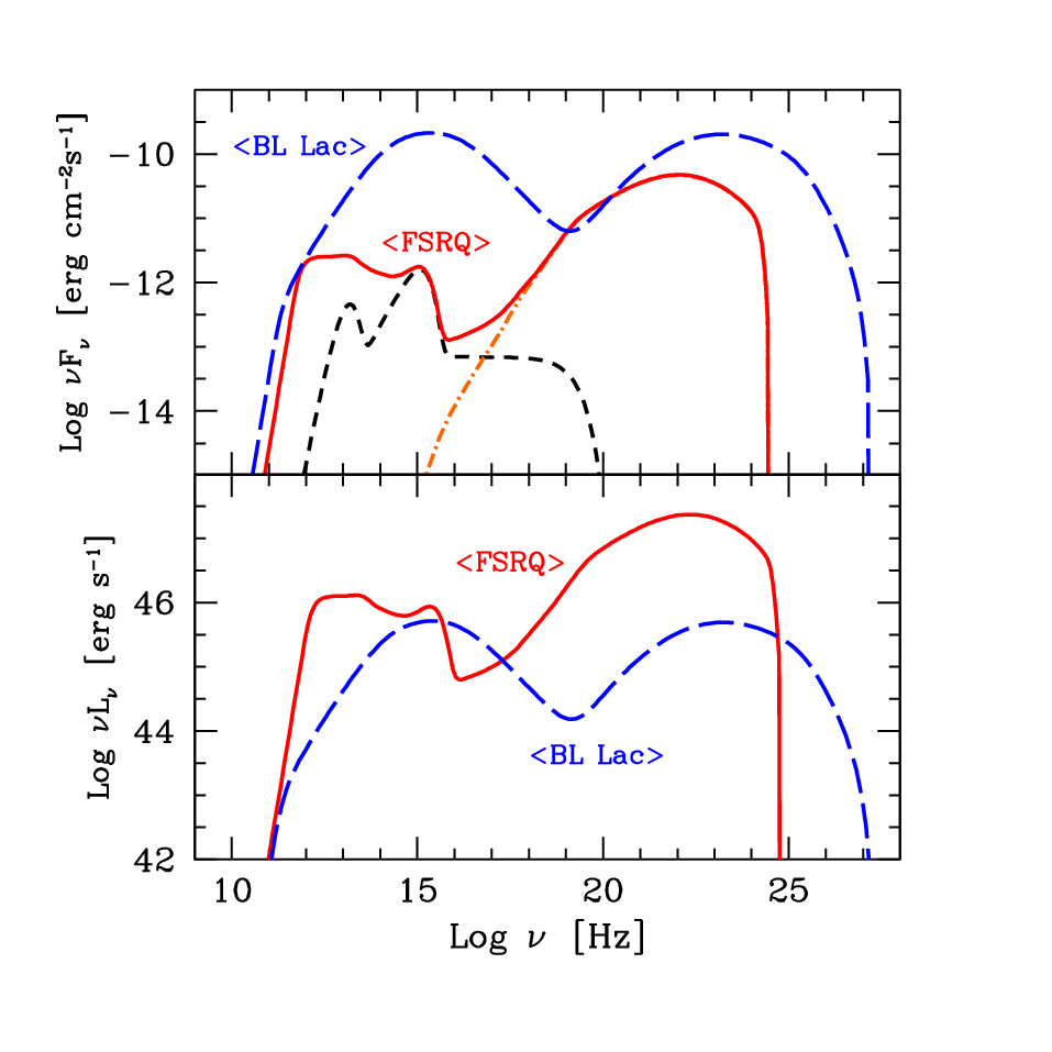
Having the distribution of all relevant physical parameters, we can do the exercise to construct the “average” SED of FSRQs and BL Lacs, respectively, of our sample. This is illustrated by Fig. 9, for which we have used for the average FSRQs and BL Lacs the parameters listed at the end of Tab. 4. Note that in our sample there are no “extreme” TeV BL Lacs, since, as discussed in T09, these sources have so large Compton peak frequencies to make difficult a detection by Fermi. So Fig. 9 corresponds to the average BL Lac detected by Fermi, and not to the average BL Lac in general.

9.2 Jet power and accretion
The jet powers derived here are large, reaching, at the high end of their distributions, values greater than 10 times the disk luminosity (see the upper panel of Fig. 10). For these extreme objects . This is admittedly a model–dependent statement. It assumes a one–zone leptonic model and that there is one proton per emitting electron. A more robust statement is that the amount of power the jet spends to produce and carry the non–thermal radiation is also very large, being in some case equal to the disk luminosity produced by accretion (see the bottom panel of Fig. 10), and more often a factor 3–10 smaller. Consider that the jet power cannot be simply be represented by : if this were the case, the entire jet power is used to produce the radiation we see, so that the jet would decelerate significantly. Instead, the jet must continue to be relativistic up to large distances, as required by the existence of strong radio lobes and the X–ray radiation seen by the Chandra satellite at distances (from the black hole) of hundreds of kpc. Therefore a reasonable lower limit on should be a factor 3–10 greater than .
What is then the source of the power of the jet? Is it only the gravitational energy of the accreting matter or do we necessarily need also the rotational energy of a spinning black hole? We here discuss two possible alternatives, that can both explain our results, but are drastically different for the ultimate energy source for the jet.
Jets powered by accretion only — Jolley et al. (2009), building up on previous ideas put forward in Jolley & Kuncic (2008), propose that, in jetted sources, a sizeable fraction of the accretion power goes to power the jet. As a result, the remaining power for the disk luminosity is less than usually estimated by setting , with –0.1. This implies that the mass accretion rate needed to sustain a given is larger than what we have estimated. Also the total accretion power is larger, and it is sufficient to explain the large jet power we have derived. Assume that the total power extractable from the accretion process is , and that a fraction () of is used to produce the disk luminosity (the jet power). We have:
| (6) |
Our results imply i) and ii) that const in different blazars to account for the observed – correlation.
Jets powered by the black hole spin — The rotational energy of a maximally spinning black hole is 29% of the hole rest mass energy (i.e. up to erg), amply sufficient to power a strong jet for its entire lifetime. In principle, in this case one can have , given a sufficiently efficient way to extract the energy of the spinning black hole. In this case we can “decouple” and , since they have a different energy source.
On the other hand, for FSRQs, we do see a relation between the and , and at first glance this seems to suggest that it is the accretion, not the spin, to power the jet. We can envisage a possible solution to this apparently contradictory issue, by linking the extraction of the hole rotational energy to the accretion process. The main idea is the following: the energy density of the accreting material close to the black hole horizon can sustain a maximum magnetic energy density of the same order (see also Ghisellini & Celotti 2002). Here is the circular (keplerian) velocity of the matter. The magnetic field sustained by the accreting matter can then tap the rotational energy of the hole. The mechanism able to do this task is the Blandford–Znajek (1977) process (hereafter BZ), whose efficiency has been debated in recent years (e.g. Moderski & Sikora 1996; Ghosh & Abramowicz 1997; Livio, Ogilvie & Pringle 1999; McKinney 2005; Garofalo 2009; Krolik & Hawley 2002). Here, for simplicity, without entering in the technical discussion on the efficiency of this mechanism, we assume that the jet power is of the form:
| (7) |
where is the dimension–less angular momentum of the hole, is some fiducial distance of the order of the black hole horizon, and is the magnetic field at that radius. Eq. 7 is nothing else than a Poynting flux. The factor includes our uncertainties about the efficiency of the BZ process.
Assume that at a distance from the black hole, the disk has a height above the equatorial plane. If is the radial in–fall velocity, we have
| (8) |
If the energy density of the magnetic field is a fraction of the kinetic energy density of the matter orbiting around the black hole, we have
| (9) |
If a magnetic field with the same magnitude is threading the spinning hole, then we have
| (10) |
Close to the gravitational or Schwarzschild radius, we may set . The ratio can be slightly larger than unity, depending on viscosity. For , the jet power is maximum, and for not much less than unity can be of the same order of the disk luminosity. The (rather strong) requirement that our data are posing on the BZ mechanism is therefore on its efficiency, that must be large.
Acknowledgments
This work was partly financially supported by a 2007 COFIN–MIUR and an ASI I/088/06) grant. This research made use of the NASA/IPAC Extragalactic Database (NED) which is operated by the Jet Propulsion Laboratory, Caltech, under contract with the NASA. We acknowledge the use of public data from the Swift data archive. The research made use of data obtained from the High Energy Science Archive Research Center (HEASARC), provided by NASA’s GSFC.
References
- [] Abdo A.A., Ackermann M., Ajello M., et al., 2009a, ApJ, 700, 597 (A09)
- [] Abdo A.A., Ackermann M., Ajello M., et al., 2009b, ApJ, 699, 976
- [] Aharonian F., Akhperjanian A.G., Razer–Bachi A.R. et al., 2007, ApJ, 664, L71
- [] Albert J., et al., 2007, ApJ, 669, 862
- [] Barth A.J., Ho L.C. & Sargent W.L.W., 2003, ApJ, 583, 134
- [] Blandford R.D. & Znajek R.L., 1977, MNRAS, 179, 433
- [] Błazejowski M., Sikora M., Moderski R. & Madejski G.M., 2000, ApJ, 545, 107
- [] Böttcher M. & Dermer C.D., 2002, ApJ, 564, 86
- [] Cardelli J.A., Clayton G.C. & Mathis J.S., 1989, ApJ, 345, 245
- [] Cavaliere A. & D’Elia V., 2002, ApJ, 571, 226
- [] Celotti A. & Ghisellini G., 2008, MNRAS, 385, 283
- [] Chen Z., Gu M., Fan Z. & Cao X., 2009, Research in Astr. Astrophys., in press (astro–ph/0906.3373)
- [] Falomo R., Kotilainen J.K., Carangelo N. & Treves A., 2003a, ApJ, 595, 624
- [] Falomo R., Carangelo N. & Treves A., 2003b, MNRAS, 343, 505
- [] Fichtel C.E., Bertsch J., Chiang J. et al., 1994, ApJS, 94, 551
- [] Foschini L. et al. 2009, Proceedings of the Conference ”Accretion and Ejection in AGN: a global view”, in press (astro–ph/0908.3313)
- [] Fossati G., Maraschi L., Celotti A., Comastri A. & Ghisellini G., 1998, MNRAS, 299, 433
- [] Garofalo D., 2009, ApJ, 699, 400
- [] Georganopoulos M. & Kazanas D., 2003, ApJ, 594, L27
- [] Ghisellini G., Celotti A., Fossati G., Maraschi L. & Comastri A., 1998, MNRAS, 301, 451
- [] Ghisellini G. & Celotti A., 2001, MNRAS, 327, 739
- [] Ghisellini G. & Celotti A., 2002, in “Blazar Astrophysics with BeppoSAX and Other Observatories” workshop, Editors: P. Giommi, E. Massaro, G. Palumbo. ESA–ESRIN, p. 257.
- [] Ghisellini G. & Tavecchio F., 2008, MNRAS, 386, L28
- [] Ghisellini G., Foschini L., Volonteri M., Ghirlanda G., Haardt F., Burlon D., Tavecchio F. 2009a, MNRAS, 399, L24
- [] Ghisellini G., Tavecchio F., Bodo G. & Celotti A., 2009b, MNRAS, 393, L16
- [] Ghisellini G., Maraschi L. & Tavecchio F., 2009, MNRAS, 396, L105
- [] Ghisellini G., Tavecchio F. & Ghirlanda G., 2009, MNRAS, in press (Paper 1)
- [] Ghisellini G. & Tavecchio F., 2009, MNRAS, 397, 985 (GT09)
- [] Ghosh P. & Abramowicz M.A., 1997, MNRAS, 292, 887
- [] Giannios D., Uzdensky D.A. & Begelman M.C., 2009, MNRAS, 395, L29
- [] Ho L., 2008, ARA&A, 46, 475
- [] Ho L., 2009, ApJ, 699, 626
- [] Jauncey D.L., Savage A., Morabito D.D., Preston R.A., Nicolson G.D. & Tzioumis A.K. 1989, AJ, 98, 54
- [] Jolley E.J.D. & Kuncic Z., 2008, MNRAS, 386, 989
- [] Jolley E.J.D., Kuncic Z., Bicknell G.V. & Wagner S., 2009, MNRAS, in press (astro–ph/0908.2337)
- [] Kalberla P.M.W., Burton W.B., Hartmann D., Arnal E.M., Bajaja E., Morras R. & Pöppel W.G. L. 2005, A&A, 440, 775
- [] Kataoka J., Stawarz Ł., 2005, ApJ, 622, 797
- [] Kataoka J., et al., 2008, ApJ, 685, 839
- [] Krolik J.H. & Hawley J.F., 2002, ApJ, 573, 754
- [] Liu Y., Jiang D.R. & Gu F., 2006, ApJ 637, 669
- [] Liu Y., Jiang D.R. & Gu M.F., 2009, ApJ, 637, 669
- [] Livio M., Ogilvie G.I. & Pringle J.R., 1999, ApJ, 512, 100
- [] Maraschi L. & Tavecchio F., 2003, ApJ, 593, 667
- [] McKinney J.C., 2005, ApJ, 630, L5
- [] Moderski R. & Sikora M., 1996, MNRAS, 283, 854
- [] Padovani P., 1992, A&A, 256, 399
- [] Piner B.G. & Edwards P.G., 2004, ApJ, 600, 115
- [] Piner B.G., Pant N. & Edwards P.G., 2008, ApJ, 678, 64
- [] Pian E., Falomo R., & Treves A., 2005, MNRAS, 369, 919
- [] Poole T.S., Breeveld A.A., Page M.J. et al., 2008, MNRAS, 383, 627
- [] Roming P.W.A., Kennedy T.E., Mason K.O., et al., 2005, Space Sci. Rev., 120, 95
- [] Sambruna R.M., Gliozzi M., Tavecchio F. et al., 2006, ApJ, 652, 146
- [] Schlegel D.J., Finkbeiner D.P. & Davis M., 1998, ApJ, 500, 525
- [] Shakura N.I. & Syunyaev, R.A., 1973, A&A, 24, 337
- [] Sikora M., Begelman M.C. & Rees M.J., 1994, ApJ, 421, 153
- [] Sikora M., Błazejowski M., Moderski R. & Madejski G.M., 2002, ApJ, 577, 78
- [] Tavecchio F., Maraschi L. & Ghisellini G., 1998, ApJ, 509, 608
- [] Tavecchio F., Maraschi L., Sambruna R.M., Urry C.M., Cheung C.C., Gambill J.K. & Scarpa R., 2004, ApJ, 614, 64
- [] Tavecchio F., Maraschi L., Ghisellini G., Kataoka J., Foschini L., Sambruna R.M. & Tagliaferri G., 2007, ApJ, 665, 980
- [] Tavecchio F., Ghisellini G., Ghirlanda G., Foschini L. & Maraschi L., 2009, MNRAS, in press (astro–ph/0909.0651) (T09)
- [] Vlahakis N. & Königl A., 2004, ApJ, 605, 656
- [] Wagner R.M., 2008, MNRAS, 385, 119
- [] Wang J–M., Luo B. & Ho L.C., 2004, ApJ, 615, L9
- [] Woo J–H., Urry C.M., van der Marel R.P., Lira P. & Maza J., 2005, ApJ, 631, 762
- [] Worrall D.M., Birkinshaw M. & Hardcastle M.J., 2001, MNRAS, 326, L7
- [] Wu X.–B., Liu F.K. & Zhang T.Z., 2002, A&A 389, 742
- [] Xie G.Z., Liu H.T., Cha G.W., Ma L., Xie Z.H. & Chen L.E., 2005, AJ 130, 2506
- [] Xu Y.-D., Cao X. & Wu Q., 2009, ApJ, 694, L107
10 appendix: Spectral Energy Distributions


