The description of physical quantities has been widely developed in theory based on the action principle. The strength and the form of interactions affect physical quantities involving virtual processes by quantum loop corrections. It is a key ingredient how interactions are taken into account in the action integral. As a principle, theory has invariance such as Poincaré invariance. Because invariances of a theory lead to conserved currents, they are significant constraints.

Renormalizability is another important element of a restriction to theory. Once a finite number of all the renormalizable interactions are written down, new counterterms are not required. This makes perturbation valid. On the other hand, invariance of theory such as Poincaré invariance does not have a crucial role to forbid non-renormalizable interactions. If a non-renormalizable interaction is added, new counterterms would be needed. The new terms would give rise to the corresponding contributions and the number of counterterms can be infinite. Renormalizability seems to be additional requirement in perturbation. In extracting physical quantities, however, renormalizability is not compulsory from the point of view that non-renormalizable interactions are irrelevant operators and that the contributions to physical quantities are negligible. In four dimensions, usually non-renormalizable interactions are supposed to be suppressed by an ultraviolet momentum cutoff of a theory. Effective theory with a large cutoff can be predictable without requiring renormalizability.

It is nontrivial whether only four-dimensional theory is privileged to yield physical accuracy in a non-renormalizable theory. A characteristic property in four dimensions is that renormalizable and non-renormalizable interactions coexist. In a theory with compactified extra dimensions, fields as four-dimensional modes can have dimension-four operators which are similar to renormalizable terms in four dimensions. If coefficients of other operators are small, such a theory might be predictable with a certain accuracy. The coefficients of higher dimensional operators are unknown and should be eventually determined. For addressing this problem, there are some attitudes. One is to try to construct a consistent theory to specify all the non-renormalizable interactions. Another is to search for rules or orders for possible interactions at each given loop level in a non-renormalizable theory. In this paper, our standing point is to aim for identifying contributions of higher-dimensional operators appearing at two-loop level.

Since new frameworks for solving the hierarchy problem have been proposed [1, 2], quantum loop corrections of interactions in a bulk have been studied in various models with compactified extra dimensions. As a radical possibility, all the fields of the standard model might propagate in a bulk [3]. If gauge bosons propagate in a bulk, there is a mechanism of dynamical gauge symmetry breaking [4]. One of remarkable features in orbifold models is that loop effects of bulk fields produce infinite contributions to require renormalization by four-dimensional couplings on boundaries [5]. Boundary terms can be mass and kinetic energy terms and higher derivative operators can be needed as counterterms for loop corrections [6]-[11].

Recently, higher derivative terms have been utilized for a phenomenologically accessible idea in the Lee-Wick standard model [12]. Here the higher derivative propagator contains two poles and a cancellation between contributions from the two poles removes the quadratic divergence associated with the Higgs mass. In the context of large extra dimensions, it has been shown that a new type of divergence which corresponds to a higher derivative operator is generated by quantum corrections from the exchange of virtual Kaluza-Klein gravitons [13]. It gives an explanation for solving the hierarchy problem as an ultraviolet cutoff of the theory is the TeV scale. Aspects such as subtlety about massive ghost fields have also been discussed in this model [14]. The scenario of the Lee-Wick standard model is interesting but the effect of higher derivative operators seems comparable to that of dimension-four operators. In this paper, we pursue a conventional approach based on such a view that irrelevant operators are small in an effective theory while we treat poles of propagators in a way developed in the Lee-Wick standard models.

We calculate quantum loop corrections to two-point functions in a five-dimensional $\phi^{4}$ theory on an orbifold $S^{1}/Z_{2}$. As in four dimensions, divergences for mass terms and wave fucntions are found at one-loop and two-loop levels, respectively At two-loop level, we find that divergence for quartic derivative terms of $(p^{2})^{2}$ appears for the bulk. The counterterms are needed and these terms make propagators have two poles. With this effect taken into account, corrections to two-point functions are derived. The contributions of the quartic derivative terms to masses depend on both of an ultraviolet cutoff denoted as $\Lambda$ and a size of an extra dimension denoted as $L$. We show that the contributions can be extracted with a moderate fine-tuning for $\Lambda L\hskip 3.00003pt\raisebox{1.72218pt}{$>$}\hskip-7.5pt\raisebox{-3.01385pt}{$\sim$}\hskip 3.00003pt10^{2}$ and that they cannot be fixed for $\Lambda L\sim 10$. Therefore, for extraction of physical quantities for two-point functions an ultraviolet cutoff must be orders of magnitude larger compared to a compactification scale. This behavior is in agreement with the conventional observation that contributions of higher-dimensional operators are small for a large cutoff.

We also discuss corrections with multiple poles at higher loop levels. An example of higher derivative terms beyond $(p^{2})^{2}$ is given at four-loop level. It is found that a similar large cutoff tends to be needed.

The paper is organized as follows. In Sec. 2, we present our model including fields and action integrals. In Sec. 3, two-point functions at tree and one-loop levels are given. In Sec. 4, we calculate quantum corrections for two-point functions at two-loop level. It is found that divergence of $(p^{2})^{2}$ terms appears. In Sec. 5, by starting with the action integral including $(p^{2})^{2}$ terms, we derive corrections for two-point functions. Here dependence of the corrections on $\Lambda L$ is given. In Sec. 6, higher-loop corrections are discussed. An exemplification is given at four-loop level. We conclude in Sec. 7 with some remarks. Details of calculations and formulas are shown in appendices.

We start with the action for the real scalar field $\phi(x,y)$,

$\displaystyle S$

$\displaystyle\!\!\!=\!\!\!$

$\displaystyle\int d^{4}x\int_{0}^{L}dy\left({1\over 2}(\partial_{\mu}\phi)^{2}-{1\over 2}(\partial_{y}\phi)^{2}-{1\over 2}m^{2}\phi^{2}-\lambda_{5}\phi^{4}\right).$

(2.1)

Greek indices $\mu$ run over 0,1,2,3 and fifth index is denoted as $y$. We use a metric $\eta_{\mu\nu}=\textrm{diag}(1,-1,-1,-1)$. The extra-dimensional space is compactified on $S^{1}/Z_{2}$, where the fundamental region is $0\leq y\leq L$. The five-dimensional spacetime is flat. The boundary conditions for the scalar $\phi(x,y)$ are

$\displaystyle\phi(x,-y)=\phi(x,y),\qquad\phi(x,L-y)=\phi(x,L+y).$

(2.2)

The mode expansion is given by

$\displaystyle\phi(x,y)$

$\displaystyle\!\!\!=\!\!\!$

$\displaystyle\sqrt{1\over L}\,\phi_{0}(x)+\sum_{n=1}^{\infty}\sqrt{2\over L}\,\cos\left(m_{n}y\right)\phi_{n}(x),$

(2.3)

where the mass for $\phi_{n}(x)$ is $m_{n}={n\pi\over L}$. In calculating loop corrections, it is convenient to employ $-\infty\leq n\leq\infty$ for a sum with respect to $n$. Eq. (2.3) is rewritten as

$\displaystyle\phi(x,y)$

$\displaystyle\!\!\!=\!\!\!$

$\displaystyle\sqrt{1\over 2L}\left((\sqrt{2}-1)\phi_{0}(x)+\sum_{n=-\infty}^{\infty}\cos\left(m_{n}y\right)\phi_{|n|}(x)\right).$

(2.4)

Substituting this equation into the action (2.1) leads to

	$\displaystyle S$	$\displaystyle\!\!\!=\!\!\!$	$\displaystyle\int d^{4}x\left\{{1\over 2}(\partial_{\mu}\phi_{0})^{2}-{1\over 2}m^{2}\phi_{0}^{2}+\sum_{n=1}^{\infty}\left({1\over 2}(\partial_{\mu}\phi_{n})^{2}-{1\over 2}(m^{2}+m_{n}^{2})\phi_{n}^{2}\right)\right.$		(2.5)
			$\displaystyle-{\lambda_{5}\over 4L}\left(\left((\sqrt{2}-1)^{4}+4(\sqrt{2}-1)^{3}\right)\phi_{0}^{4}\right.+6(\sqrt{2}-1)^{2}\sum_{n=-\infty}^{\infty}\phi_{0}^{2}\phi_{|n|}^{2}$
			$\displaystyle+4(\sqrt{2}-1)\sum_{n=-\infty}^{\infty}\sum_{\ell=-\infty}^{\infty}\phi_{0}\phi_{|n|}\phi_{|\ell|}\phi_{|n+\ell|}\left.\left.+\sum_{n=-\infty}^{\infty}\sum_{\ell=-\infty}^{\infty}\sum_{s=-\infty}^{\infty}\phi_{|n|}\phi_{|\ell|}\phi_{|s|}\phi_{|n+\ell+s|}\right)\right\},$

where the kinetic energy and mass terms are denoted as the sum of zero mode and modes $1\leq n\leq\infty$ so that the modes of quadratic terms correspond to degrees of freedom of propagation. Here $\lambda\equiv\lambda_{5}/L$ is dimensionless. Infinite sum with respect to modes is the effect of the five-dimensional origin. Even if there are only dimension-two and dimension-four operators, the five-dimensional effect gives rise to new divergent terms, as we will see. The interaction terms have invariance under $n\leftrightarrow-n$. The quadratic terms of scalars are diagonal with respect to modes $n$.

At boundaries, $\phi^{2}$ are expanded as

	$\displaystyle\left.\phi^{2}\right|_{y=0}$	$\displaystyle\!\!\!=\!\!\!$	$\displaystyle{1\over 2L}\left((\sqrt{2}-1)^{2}\phi_{0}^{2}+2(\sqrt{2}-1)\sum_{n=-\infty}^{\infty}\phi_{0}\phi_{|n|}+\sum_{n=-\infty}^{\infty}\sum_{\ell=-\infty}^{\infty}\phi_{|n|}\phi_{|\ell|}\right),$		(2.6)
	$\displaystyle\left.\phi^{2}\right|_{y=L}$	$\displaystyle\!\!\!=\!\!\!$	$\displaystyle{1\over 2L}\left((\sqrt{2}-1)^{2}\phi_{0}^{2}+2(\sqrt{2}-1)\sum_{n=-\infty}^{\infty}(-1)^{n}\phi_{0}\phi_{|n|}\right.$		(2.7)
			$\displaystyle\left.+\sum_{n=-\infty}^{\infty}\sum_{\ell=-\infty}^{\infty}(-1)^{n+\ell}\phi_{|n|}\phi_{|\ell|}\right).$

From this equation, quadratic terms at boundaries are

			$\displaystyle\int_{0}^{L}dy\,\phi^{2}\left(\delta(y)+\delta(y-L)\right)$		(2.8)
		$\displaystyle\!\!\!=\!\!\!$	$\displaystyle{1\over L}\left((\sqrt{2}-1)^{2}\phi_{0}^{2}+2(\sqrt{2}-1)\sum_{n=-\infty}^{\infty}\phi_{0}\phi_{|2n|}+\sum_{n=-\infty}^{\infty}\sum_{s=-\infty}^{\infty}\phi_{|n|}\phi_{|n+2s|}\right),$

which have non-diagonal components with respect to modes $n$.

By a dimensional analysis with $[\phi]=[\textrm{mass}]^{3\over 2}$ and $[\lambda_{5}]=[\textrm{mass}]^{-1}$, possible Lagrangian counterterms are expected in terms of power of $\lambda_{5}$ as

$\displaystyle(\partial\phi)^{2},~~\lambda_{5}\phi^{4},~~\lambda_{5}^{2}(\partial^{2}\phi)^{2},~~\lambda_{5}^{3}(\partial\phi)^{2}\phi^{2},~~\lambda_{5}^{4}\phi^{6},~~\lambda_{5}^{4}(\partial^{3}\phi)^{2},~~\lambda_{5}^{6}(\partial\phi)^{2}\phi^{4},~~\cdots,$

(2.9)

where vector indices are contracted.

At tree level, the two-point functions for $\phi_{0}(x)\phi_{0}(x)$ and $\phi_{n}(x)\phi_{n}(x)$ are

	$\displaystyle D(x-w)$	$\displaystyle\!\!\!=\!\!\!$	$\displaystyle\int{d^{4}p\over(2\pi)^{4}}\,{i\over p^{2}-m^{2}+i\epsilon}\,e^{-ip\cdot(x-w)},$		(3.1)
	$\displaystyle D_{n}(x-w)$	$\displaystyle\!\!\!=\!\!\!$	$\displaystyle\int{d^{4}p\over(2\pi)^{4}}\,{i\over p^{2}-m^{2}-m_{n}^{2}+i\epsilon}\,e^{-ip\cdot(x-w)},$		(3.2)

respectively. We will omit $i\epsilon$ hereafter.

The diagram for one-loop two-point functions is shown in Fig. 1.

Here external lines can take $\phi_{0}$ or $\phi_{|n|}$. One-loop amplitudes are calculated from

$\displaystyle\left\langle\phi_{0}(x)\phi_{0}(w)\,i\int d^{4}x\,{\cal L}\right\rangle,\quad\left\langle\phi_{0}(x)\phi_{|f|}(w)\,i\int d^{4}x\,{\cal L}\right\rangle,\quad\left\langle\phi_{|f|}(x)\phi_{|g|}(w)\,i\int d^{4}x\,{\cal L}\right\rangle.$

(3.3)

We obtain the one-loop contribution for the two-point function with the external lines $\phi_{|f|}\phi_{|g|}$ as

	$\displaystyle\tilde{G}_{|f||g|}$	$\displaystyle\!\!\!=\!\!\!$	$\displaystyle-3i\lambda\bigg((\sqrt{2}-1)^{2}\delta_{f0}\delta_{g0}{\cal D}+\delta_{f0}\delta_{g0}\sum_{n=-\infty}^{\infty}{\cal D}_{n}+\,\delta_{|f||g|}\sum_{n=-\infty}^{\infty}{\cal D}_{n}$		(3.4)
			$\displaystyle+(\sqrt{2}-1)\,\sum_{n=-\infty}^{\infty}\left(\delta_{f0}\delta_{|g||2n|}+\delta_{g0}\delta_{|f||2n|}\right){\cal D}_{n}+\sum_{n=-\infty}^{\infty}\delta_{|f||g+2n|}{\cal D}_{n}\bigg).$

Here the two momentum integrals are given as

$\displaystyle{\cal D}=\int{d^{4}k\over(2\pi)^{4}}\,{i\over k^{2}-m^{2}},\qquad{\cal D}_{n}=\int{d^{4}k\over(2\pi)^{4}}\,{i\over k^{2}-m^{2}-m_{n}^{2}}.$

(3.5)

The twp-point functions with the external lines $\phi_{0}\phi_{0}$ and $\phi_{0}\phi_{|f|}$ can be derived as limits of $\phi_{|f|}\phi_{|g|}$. The details of calculations for derivation of Eq. (3.4) are given in App. A. A note given in contraction with respect to $n$ is that $\sum_{n=-\infty}^{\infty}\delta_{|\ell||n|}\delta_{|s||n|}\neq\delta_{|\ell||s|}$. Here

$\displaystyle\sum_{n=-\infty}^{\infty}\delta_{|\ell||n|}\delta_{|s||n|}=2(\delta_{\ell s}+\delta_{\ell,-s})-3\delta_{\ell 0}\delta_{s0},\qquad\delta_{|\ell||s|}=\delta_{\ell s}+\delta_{\ell,-s}-\delta_{\ell 0}\delta_{s0}.$

(3.6)

Now we evaluate the one-loop contribution (3.4) as Lagrangian terms of interactions. Multiplying $\tilde{G}_{|f||g|}$ by $\phi_{|f|}\phi_{|g|}$ and summing with respect to $f,g$ lead to

	$\displaystyle\sum_{f=-\infty}^{\infty}\sum_{g=-\infty}^{\infty}\phi_{|f|}\phi_{|g|}\tilde{G}_{|f||g|}=-3i\lambda\left((\sqrt{2}-1)^{2}\phi_{0}^{2}{\cal D}+2(\sqrt{2}-1)\sum_{n=-\infty}^{\infty}\phi_{0}\phi_{|2n|}{\cal D}_{n}\right.$
	$\displaystyle\qquad\qquad+\sum_{f=-\infty}^{\infty}\sum_{n=-\infty}^{\infty}\phi_{|f|}\phi_{|f+2n|}{\cal D}_{n}\left.+\left(\phi_{0}^{2}+\sum_{\ell=-\infty}^{\infty}\phi_{|\ell|}^{2}\right)\sum_{n=-\infty}^{\infty}{\cal D}_{n}\right).$		(3.7)

This one-loop corrections include bulk and boundary divergences.

A bulk mass term is expanded as

$\displaystyle-\int_{0}^{L}dy\,m^{2}\phi^{2}=-{1\over 2}m^{2}\left(\phi_{0}^{2}+\sum_{\ell=-\infty}^{\infty}\phi_{|\ell|}^{2}\right).$

(3.8)

From Eq. (3.7), bulk divergent terms at one-loop level are

$\displaystyle\left(\phi_{0}^{2}+\sum_{\ell=-\infty}^{\infty}\phi_{|\ell|}^{2}\right)\sum_{n=-\infty}^{\infty}{\cal D}_{n}.$

(3.9)

The divergent part of the integral is

$\displaystyle\left.\sum_{n=-\infty}^{\infty}{\cal D}_{n}\right|_{\textrm{\scriptsize div}}={1\over 2^{4}\pi^{5\over 2}}\left({2\over 3}\Lambda^{2}-2m^{2}\right)\Lambda L.$

(3.10)

The details of calculations are given in App. B. From Eqs. (3.9) and (3.10), the bulk divergent term at one-loop level is obtained as

$\displaystyle{1\over 2^{2}\pi^{5\over 2}}\int_{0}^{L}dy\,\left({1\over 3}\Lambda^{2}-m^{2}\right)\Lambda L\phi^{2}.$

(3.11)

The divergence of $\Lambda^{3}$ is expected from a five-dimensional integral of a propagator,

$\displaystyle\sum_{n=-\infty}^{\infty}\int{d^{4}k\over(2\pi)^{4}}{i\over k^{2}-m^{2}-m_{n}^{2}}\to\int{d^{5}\bar{k}\over(2\pi)^{5}}{i\over\bar{k}^{2}-m^{2}}\sim\Lambda^{3},$

(3.12)

where $\bar{k}=(k,k_{y})$.

In Eq. (3.7), the other divergent terms have contractions between external mode indices and internal mode indices. The sum with respect to modes is not independent of external lines. It is regarded as the structure that each mode has four-dimensional divergence,

	$\displaystyle\int{d^{4}k\over(2\pi)^{4}}\,{i\over k^{2}-m_{n}^{2}-M^{2}}$	$\displaystyle\!\!\!=\!\!\!$	$\displaystyle{1\over 16\pi^{2}}\int_{0}^{\Lambda^{2}}d(k_{E}^{2})\,{k_{E}^{2}\over k_{E}^{2}+m_{n}^{2}+M^{2}}$		(3.13)
		$\displaystyle\!\!\!=\!\!\!$	$\displaystyle{1\over 16\pi^{2}}\left(\Lambda^{2}-(m_{n}^{2}+M^{2})\log{\Lambda^{2}\over m_{n}^{2}+M^{2}}\right),$

where $M=m$ for ${\cal D}_{n}$.

From Eq. (2.8), boundary terms including $\partial_{y}$ are

			$\displaystyle\int_{0}^{L}dy\,{1\over 4}\left(\partial_{y}^{2}\phi\cdot\phi+\phi\partial_{y}^{2}\phi-2\partial_{y}\phi\partial_{y}\phi\right)\left(\delta(y)+\delta(y-L)\right)$		(3.14)
		$\displaystyle\!\!\!=\!\!\!$	$\displaystyle-{1\over 4L}\left(\sum_{f}\sum_{n}\left(m_{f}-m_{f+2n}\right)^{2}\phi_{|f|}\phi_{|f+2n|}+2(\sqrt{2}-1)\sum_{n}\left(m_{2n}^{2}\right)\phi_{0}\phi_{|2n|}\right)$
		$\displaystyle\!\!\!=\!\!\!$	$\displaystyle-{1\over L}\left(\sum_{f}\sum_{n}m_{n}^{2}\phi_{|f|}\phi_{|f+2n|}+2(\sqrt{2}-1)\sum_{n}m_{n}^{2}\phi_{0}\phi_{|2n|}\right).$

From this equation and Eq. (2.8), the boundary terms in one-loop two-point function corresponds to

			$\displaystyle\int_{0}^{L}dy\,\left\{-m^{2}\phi^{2}+{1\over 4}\left(\partial_{y}^{2}\phi\cdot\phi+\phi\partial_{y}^{2}\phi-2\partial_{y}\phi\partial_{y}\phi\right)\right\}\left(\delta(y)+\delta(y-L)\right)$		(3.15)
		$\displaystyle\!\!\!=\!\!\!$	$\displaystyle-{1\over L}\left((\sqrt{2}-1)^{2}m^{2}\phi_{0}^{2}+2(\sqrt{2}-1)\sum_{n=-\infty}^{\infty}\left(m^{2}+m_{n}^{2}\right)\phi_{0}\phi_{|2n|}\right.$
			$\displaystyle\left.+\sum_{f=-\infty}^{\infty}\sum_{n=-\infty}^{\infty}\left(m^{2}+m_{n}^{2}\right)\phi_{|f|}\phi_{|f+2n|}\right).$

On the boundaries, as in a four-dimensional theory there is quadratic divergence for mass terms.

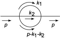
At two-loop level, there are two one-particle irreducible diagrams shown in Fig. 2.

In Fig. 2(a), the internal loops are independent of the external momentum $p$. This means that the diagram does not contribute to wave functions and higher derivative terms. At one-loop level, mass terms have been introduced for both of bulk and boundary Lagrangian terms. We will not discuss this diagram further.

The two-loop diagram we calculate is the diagram drawn in Fig. 2(b). The amplitude is calculated from

$\displaystyle\left\langle\phi\phi\left(-{1\over 2}\right)\int d^{4}x_{1}{\cal L}\cdot\int d^{4}x_{2}{\cal L}\right\rangle.$

(4.1)

The last term in the action (2.5) yield the contribution to the diagram in Fig. 2(b),

			$\displaystyle\left\langle\phi_{|f|}(x)\phi_{|g|}(y)\left(-{1\over 2}\right)\left(-{\lambda\over 4}\right)^{2}\int d^{4}x_{1}\phi_{|n|}\phi_{|\ell|}\phi_{|s|}\phi_{|n+\ell+s|}\int d^{4}x_{2}\phi_{|a|}\phi_{|b|}\phi_{|c|}\phi_{|a+b+c|}\right\rangle$		(4.2)
		$\displaystyle\!\!\!\stackrel{{\scriptstyle\textrm{\scriptsize Fig.}}}{{=}}\!\!\!$	$\displaystyle-6\lambda^{2}\int d^{4}x_{1}d^{4}x_{2}\,\delta_{|f||n|}\,\delta_{|g||a|}\,\delta_{|\ell||b|}\,\delta_{|s||c|}\,\delta_{|n+\ell+s||a+b+c|}\,D_{f}D_{g}D_{\ell}D_{s}D_{n+\ell+s}$
		$\displaystyle\!\!\!\equiv\!\!\!$	$\displaystyle\tilde{G}_{|f||g|}(p)\tilde{D}_{f}(p)\tilde{D}_{g}(p),$

where the propagator $D_{f}$ is given in Eq. (3.2) and its Fourier transformation is given by $\tilde{D}_{f}(p)=i/(p^{2}-m^{2}-m_{f}^{2})$. Expansion of products of Kronecker $\delta$ is shown in Appendix C. The corresponding Lagrangian terms are obtained as

			$\displaystyle\sum_{f=-\infty}^{\infty}\sum_{g=-\infty}^{\infty}\phi_{|f|}\phi_{|g|}\tilde{G}_{|f||g|}$		(4.3)
		$\displaystyle\!\!\!=\!\!\!$	$\displaystyle-6\lambda^{2}\sum_{\ell=-\infty}^{\infty}\sum_{s=-\infty}^{\infty}\int{d^{4}k_{1}\over(2\pi)^{4}}\int{d^{4}k_{2}\over(2\pi)^{4}}\,\tilde{D}_{\ell}(k_{1})\tilde{D}_{s}(k_{2})$
			$\displaystyle\times\left[\sum_{f=-\infty}^{\infty}8\left(\tilde{D}_{f+\ell+s}\phi_{|f|}\phi_{|f|}+\tilde{D}_{f+\ell+s}\phi_{|f|}\phi_{|f+2(\ell+s)|}+2\tilde{D}_{f+\ell+s}\phi_{|f|}\phi_{|f+2s|}\right)\right.$
			$\displaystyle-24\tilde{D}_{0}\phi_{|\ell+s|}\phi_{|\ell+s|}-24\tilde{D}_{0}\phi_{|\ell+s|}\phi_{|s-\ell|}+24\delta_{s0}\tilde{D}_{0}\phi_{|\ell|}\phi_{|\ell|}-25\delta_{\ell 0}\delta_{s0}\tilde{D}_{0}\phi_{0}\phi_{0}$
			$\displaystyle-6\tilde{D}_{\ell+s}\phi_{0}\phi_{0}-8\tilde{D}_{\ell+s}\phi_{|2(\ell+s)|}\phi_{0}+8\tilde{D}_{0}\delta_{\ell+s,0}\phi_{0}\phi_{0}-16\tilde{D}_{\ell-s}\phi_{|2s|}\phi_{0}$
			$\displaystyle\left.+8\tilde{D}_{0}\delta_{\ell s}\phi_{|2\ell|}\phi_{0}+16\delta_{s0}\tilde{D}_{\ell}\phi_{0}\phi_{0}+16\delta_{s0}\tilde{D}_{\ell}\phi_{|2\ell|}\phi_{0}\right],$

where $\tilde{D}=\tilde{D}(p-k_{1}-k_{2})$ in the brackets. In this equation, the term with three sums of $\sum_{\ell}\sum_{s}\sum_{f}$

$\displaystyle-48\lambda^{2}\sum_{\ell=-\infty}^{\infty}\sum_{s=-\infty}^{\infty}\int{d^{4}k_{1}\over(2\pi)^{4}}\int{d^{4}k_{2}\over(2\pi)^{4}}\,\tilde{D}_{\ell}(k_{1})\tilde{D}_{s}(k_{2})\sum_{f=-\infty}^{\infty}\tilde{D}_{f+\ell+s}(p-k_{1}-k_{2})\phi_{|f|}\phi_{|f|},$

(4.4)

comes only from Eq. (4.2) among various terms in Eq. (4.1). Eq. (4.4) is the full term with three sums of $\sum_{\ell}\sum_{s}\sum_{f}$, which is related to divergent $(p^{2})^{2}$ terms.

Now we evaluate the integral

			$\displaystyle\sum_{\ell=-\infty}^{\infty}\sum_{s=-\infty}^{\infty}\int{d^{4}k_{1}\over(2\pi)^{4}}\int{d^{4}k_{2}\over(2\pi)^{4}}\,\tilde{D}_{\ell}(k_{1})\tilde{D}_{s}(k_{2})\tilde{D}_{f+\ell+s}(p-k_{1}-k_{2})$		(4.5)
		$\displaystyle\!\!\!=\!\!\!$	$\displaystyle\sum_{\ell=-\infty}^{\infty}\int{d^{4}k_{1}\over(2\pi)^{4}}\,{i\over k_{1}^{2}-m^{2}-m_{\ell}^{2}}$
			$\displaystyle\times\left(\sum_{s=-\infty}^{\infty}\int{d^{4}k_{2}\over(2\pi)^{4}}\,{i\over k_{2}^{2}-m^{2}-m_{s}^{2}}{i\over(p-k_{1}-k_{2})^{2}-m^{2}-m_{f+\ell+s}^{2}}\right),$

In order to extract dependence on an external momentum $p$, we expand momentum-dependent part of the integrand as

	$\displaystyle{1\over(p-k)^{2}-m^{2}}$	$\displaystyle\!\!\!=\!\!\!$	$\displaystyle{1\over k^{2}-m^{2}}+\left[-{1\over(k^{2}-m^{2})^{2}}+{k^{2}\over(k^{2}-m^{2})^{3}}\right]p^{2}$		(4.6)
			$\displaystyle+\left[{1\over(k^{2}-m^{2})^{3}}-{3k^{2}\over(k^{2}-m^{2})^{4}}+{2(k^{2})^{2}\over(k^{2}-m^{2})^{5}}\right](p^{2})^{2}$
			$\displaystyle+{\cal O}\left({1\over(k^{2}-m^{2})^{4}}(p^{2})^{3}\right),$

where odd $k$ has been dropped as it vanishes for $k$ integral. It will be seen that $(p^{2})^{s}~(s\geq 3)$ terms are convergent. For simplicity, we proceed the evaluation of the integral for $m=0$. The case with nonzero $m$ can be analyzed in a similar way. The $(p^{2})^{2}$ terms in Eq. (4.5) are

	$\displaystyle\sum_{\ell=-\infty}^{\infty}\sum_{s=-\infty}^{\infty}\int{d^{4}k_{1}\over(2\pi)^{4}}\int{d^{4}k_{2}\over(2\pi)^{4}}\,{i\over k_{1}^{2}-m_{\ell}^{2}}{i\over k_{2}^{2}-m_{s}^{2}}i(p^{2})^{2}$
	$\displaystyle\times\left[{1\over((k_{1}+k_{2})^{2}-m_{f+\ell+s}^{2})^{3}}-{3(k_{1}+k_{2})^{2}\over((k_{1}+k_{2})^{2}-m_{f+\ell+s}^{2})^{4}}+{2((k_{1}+k_{2})^{2})^{2}\over((k_{1}+k_{2})^{2}-m_{f+\ell+s}^{2})^{5}}\right].$
			(4.7)

From this equation, we find the divergence for $(p^{2})^{2}$ terms,

$\displaystyle i(p^{2})^{2}{L^{2}\over 105(4\pi)^{4}}\log(\Lambda^{2}L^{2}).$

(4.8)

For a calculation of the integral, equations and identities are shown in App. B.

The Lagrangian term for this $(p^{2})^{2}$ divergence is obtained by substituting Eq. (4.8) into Eq. (4.4) as

$\displaystyle-{i\over 35(2\pi)^{4}}\sum_{f=-\infty}^{\infty}\log(\Lambda^{2}L^{2})\cdot\lambda_{5}^{2}(p^{2})^{2}\phi_{|f|}\phi_{|f|}.$

(4.9)

The equation (4.9) has the sum of diagonal components with respect to mode $f$ so that the contributions are bulk terms. The divergence of $\log\Lambda$ for $(p^{2})^{2}$ terms in the bulk is expected from an interpretation of Eq. (4.7) as a five-dimensional integral,

			$\displaystyle\sum_{\ell=-\infty}^{\infty}\sum_{s=-\infty}^{\infty}\int{d^{4}k_{1}\over(2\pi)^{4}}\int{d^{4}k_{2}\over(2\pi)^{4}}\,{1\over k_{1}^{2}-m_{\ell}^{2}}{1\over k_{2}^{2}-m_{s}^{2}}{1\over((k_{1}+k_{2})^{2}-m_{f+\ell+s}^{2})^{3}}$		(4.10)
		$\displaystyle\!\!\!\to\!\!\!$	$\displaystyle\int{d^{5}\bar{k}_{1}\over(2\pi)^{5}}\int{d^{5}\bar{k}_{2}\over(2\pi)^{5}}\,{1\over\bar{k}_{1}^{2}}{1\over\bar{k}_{2}^{2}}{1\over((\bar{k}_{1}+\bar{k}_{2})^{2})^{3}}\sim\log\Lambda,$

where $\bar{k}=(k,k_{y})$. In five dimensions, the emergence of higher derivative terms as an effective field theory has also been shown in a method with a space-dependent cutoff [17, 18, 19].

Boundary terms have contractions between external mode indices and internal mode indices. The sum with respect to modes is not independent of external fields $\phi_{|s|}$. On boundaries, there is no divergence for $(p^{2})^{2}$ because the number of summation is less. Divergence for $p^{2}$ is generated on boundaries as in a four-dimensional case.

For $(p^{2})^{3}$, it is seen from Eqs. (B.11) and (B.15) that the integral to determine divergence in (4.7) reduces to $\int_{0}^{\infty}db\,e^{-Ab}$ where $A$ is a positive number. This integration converges. Similarly for $(p^{2})^{s}(s\geq 3)$, the integrals converge. This convergence is expected from an interpretation of a five-dimensional integral as in Eq. (4.10).

Because of divergence of $(p^{2})^{2}$ term, the Lagrangian must have the counterterm. In next section, we will take into account this effect on two-point functions.

In this section, we examine quantum corrections by starting with the action integral including $(p^{2})^{2}$ terms.

The action integral with $(p^{2})^{2}$ is

$\displaystyle S_{t}=S+S_{p^{4}}+S_{m^{2}}+S_{p^{2}},$

(5.1)

In addition to the action $S$ given in Eq. (2.1)

$\displaystyle S=\int d^{4}x\int_{0}^{L}dy\,\left({1\over 2}(\partial_{\mu}\phi)^{2}-{1\over 2}(\partial_{y}\phi)^{2}-{1\over 2}m^{2}\phi^{2}-\lambda_{5}\phi^{4}\right),$

(5.2)

we take into account the corresponding terms to divergences appearing at two-loop level:

	$\displaystyle S_{p^{4}}$	$\displaystyle\!\!\!=\!\!\!$	$\displaystyle\int d^{4}x\int_{0}^{L}dy\,U\left(\partial_{M}\partial_{N}\phi\cdot\partial^{M}\partial^{N}\phi\right),$		(5.3)
	$\displaystyle S_{m^{2}}$	$\displaystyle\!\!\!=\!\!\!$	$\displaystyle\int d^{4}x\int_{0}^{L}dy\,E\left[-{1\over 2}m^{2}\phi^{2}+{1\over 8}\left(\partial_{y}^{2}\phi\cdot\phi+\phi\partial_{y}^{2}\phi-2\partial_{y}\phi\partial_{y}\phi\right)\right]\delta_{b},$		(5.4)
	$\displaystyle S_{p^{2}}$	$\displaystyle\!\!\!=\!\!\!$	$\displaystyle\int d^{4}x\int_{0}^{L}dy\,K\left[-{1\over 2}(\partial_{\mu}\phi)^{2}\right]\delta_{b},$		(5.5)

where $U$, $E$ and $K$ are parameters and the sum of delta functions at the boundaries is denoted as $\delta_{b}=\delta(y)+\delta(y-L)$. The parameter $U$ corresponds to $-\lambda_{5}^{2}/(35(2\pi)^{4})\sim-2\times 10^{-5}\lambda^{2}L^{2}$ in Eq. (4.9). The variation of these action integrals are given by

	$\displaystyle\delta S$	$\displaystyle\!\!\!=\!\!\!$	$\displaystyle\int d^{4}x\int_{0}^{L}dy\,\left[\left(-\partial_{\mu}\partial^{\mu}\phi+\partial_{y}^{2}\phi-m^{2}\phi-4\lambda_{5}\phi^{3}\right)\delta\phi-\partial_{y}(\partial_{y}\phi\cdot\delta\phi)\right],$		(5.6)
	$\displaystyle\delta S_{p^{4}}$	$\displaystyle\!\!\!=\!\!\!$	$\displaystyle\int d^{4}x\int_{0}^{L}dy\,2U\left[(\partial_{\mu}\partial^{\mu}-\partial_{y})^{2}\phi\cdot\delta\phi\right.$		(5.7)
			$\displaystyle\left.+2\partial_{y}\left((\partial_{\mu}\partial^{\mu}-\partial_{y}^{2})\partial_{y}\phi\cdot\delta\phi\right)+\partial_{y}^{2}(\partial_{y}^{2}\phi\cdot\delta\phi)\right],$
	$\displaystyle\delta S_{m^{2}}$	$\displaystyle\!\!\!=\!\!\!$	$\displaystyle\int d^{4}x\int_{0}^{L}dy\,E\left[(-m^{2}+\partial_{y}^{2})\phi\cdot\delta\phi\delta_{b}\right.$		(5.8)
			$\displaystyle\!\!\!\!\!+{1\over 4}\partial_{y}\left(\phi\partial_{y}\delta\phi\cdot\delta_{b}-3\partial_{y}\phi\cdot\delta\phi\delta_{b}-\phi\cdot\delta\phi\partial_{y}\delta_{b}\right)\left.+{1\over 4}\left(4\partial_{y}\phi\cdot\partial_{y}\delta_{b}+\phi\partial_{y}^{2}\delta_{b}\right)\cdot\delta\phi\right],$
	$\displaystyle\delta S_{p^{2}}$	$\displaystyle\!\!\!=\!\!\!$	$\displaystyle\int d^{4}x\int_{0}^{L}dy\,K\left[\partial_{\mu}\partial^{\mu}\phi\cdot\delta\phi\right]\delta_{b}.$		(5.9)

The effect of the boundary kinetic terms (5.9) on the leading terms (5.6) makes mixing of Neumann and Dirichlet conditions as boundary conditions [15]. The contributions for Eqs. (5.9) and (5.6) can also be treated in a way based on hermitian property of differential operators [16]. The effect of Eq. (5.8) is similarly restrictive such that the existence of zero mode is not guaranteed [9]. Thus, these boundary terms change the solutions for mode functions. Instead of solving full solutions, we can reasonably assume the existence of the solutions as the boundary terms are regarded as perturbation.

From the above equations, bulk quadratic equation of motion is

$\displaystyle(-\partial_{\mu}\partial^{\mu}+\partial_{y}^{2}-m^{2}+2U(\partial_{\mu}\partial^{\mu}-\partial_{y}^{2})^{2})\phi=0.$

(5.10)

By Fourier transformation, this equation is written as

$\displaystyle(p^{2}-m_{n}^{2}-m^{2}+2U(p^{2}-m_{n}^{2})^{2})\phi_{n}=0.$

(5.11)

The propagator is obtained as

$\displaystyle{i\over p^{2}-m_{n}^{2}-m^{2}+2U(p^{2}-m_{n}^{2})^{2}}={i\over 2U\left[\left(p^{2}+{1\over 4U}-m_{n}^{2}\right)^{2}-{1\over 16U^{2}}(1+8Um^{2})\right]}.$

(5.12)

For $1+8Um^{2}>0$, Eq. (5.12) is

$\displaystyle{1\over\sqrt{1+8Um^{2}}}\left({i\over p^{2}+{1-\sqrt{1+8Um^{2}}\over 4U}-m_{n}^{2}}-{i\over p^{2}+{1+\sqrt{1+8Um^{2}}\over 4U}-m_{n}^{2}}\right).$

(5.13)

For the poles of the propagators, positive masses squared

$\displaystyle{1-\sqrt{1+8Um^{2}}\over 4U}<0,\qquad{1+\sqrt{1+8Um^{2}}\over 4U}<0,$

(5.14)

correspond to $U<0$. In Eq. (5.13), the second term has the unusual sign so that their degrees of freedom should decay. This requires hierarchy between masses

$\displaystyle{1-\sqrt{1-8|U|m^{2}}\over 4|U|}\ll{1+\sqrt{1-8|U|m^{2}}\over 4|U|},$

(5.15)

where the mass of the lighter degree of freedom is at least of order $m_{n}$ and $U<0$. Then the propagator (5.13) is approximately given by

$\displaystyle{i\over p^{2}-m^{2}-m_{n}^{2}}-{i\over p^{2}-{1\over 2|U|}-m_{n}^{2}}.$

(5.16)

The propagator has two poles for the masses squared $m^{2}+m_{n}^{2}$ and ${1\over 2|U|}+m_{n}^{2}$. The new pole in Eq. (5.16) is directly related to the $(p^{2})^{2}$ action (5.3). The corresponding counterterms can be employed to bring in a value at a point of energy scales. For example, it would be possible to set the new pole term to zero at one scale. In this case, the value can become nonzero at other scales. In order to make the undesirable mode decay, this value must be small. If the concept of an effective theory is fulfilled as in a four-dimensional theory where higher derivative operators are irrelevant, the coefficient may be kept small at low energies. To make a general statement on the running of higher-dimensional operators is beyond the scope of the paper. When the coefficient for the $(p^{2})^{2}$ term needs to be specified in the following, we will adopt the size we have found at two-loop level.

References

• [1] N. Arkani-Hamed, S. Dimopoulos and G. R. Dvali, Phys. Lett. B 429, 263 (1998) [arXiv:hep-ph/9803315].
• [2] L. Randall and R. Sundrum, Phys. Rev. Lett. 83, 3370 (1999) [arXiv:hep-ph/9905221]; Phys. Rev. Lett. 83, 4690 (1999) [arXiv:hep-th/9906064].
• [3] T. Appelquist, H. C. Cheng and B. A. Dobrescu, Phys. Rev. D 64, 035002 (2001) [arXiv:hep-ph/0012100].
• [4] Y. Hosotani, Phys. Lett. B 126, 309 (1983); Phys. Lett. B 129, 193 (1983); Annals Phys. 190, 233 (1989).
• [5] H. Georgi, A. K. Grant and G. Hailu, Phys. Lett. B 506, 207 (2001) [arXiv:hep-ph/0012379].
• [6] G. von Gersdorff, N. Irges and M. Quiros, Nucl. Phys. B 635, 127 (2002) [arXiv:hep-th/0204223].
• [7] H. C. Cheng, K. T. Matchev and M. Schmaltz, Phys. Rev. D 66, 036005 (2002) [arXiv:hep-ph/0204342].
• [8] M. S. Carena, T. M. P. Tait and C. E. M. Wagner, Acta Phys. Polon. B 33, 2355 (2002) [arXiv:hep-ph/0207056].
• [9] F. del Aguila, M. Perez-Victoria and J. Santiago, JHEP 0302, 051 (2003) [arXiv:hep-th/0302023].
• [10] A. Muck, L. Nilse, A. Pilaftsis and R. Ruckl, Phys. Rev. D 71, 066004 (2005) [arXiv:hep-ph/0411258].
• [11] D. M. Ghilencea, JHEP 0503, 009 (2005) [arXiv:hep-ph/0409214].
• [12] B. Grinstein, D. O’Connell and M. B. Wise, Phys. Rev. D 77, 025012 (2008) [arXiv:0704.1845 [hep-ph]].
• [13] F. Wu and M. Zhong, Phys. Rev. D 78, 085010 (2008) [arXiv:0807.0132 [hep-ph]].
• [14] A. Rodigast and T. Schuster, Phys. Rev. D 79, 125017 (2009) [arXiv:0903.3851 [hep-ph]].
• [15] C. Csaki, C. Grojean, H. Murayama, L. Pilo and J. Terning, Phys. Rev. D 69, 055006 (2004) [arXiv:hep-ph/0305237].
• [16] C. Csaki, J. Hubisz and P. Meade, arXiv:hep-ph/0510275.
• [17] A. Lewandowski, M. J. May and R. Sundrum, Phys. Rev. D 67, 024036 (2003) [arXiv:hep-th/0209050].
• [18] A. Lewandowski and M. Redi, Phys. Rev. D 68, 044012 (2003) [arXiv:hep-th/0305013].
• [19] N. Uekusa, Phys. Rev. D 68, 124009 (2003) [arXiv:hep-th/0307107].
• [20] K. R. Dienes, E. Dudas and T. Gherghetta, Phys. Lett. B 436, 55 (1998) [arXiv:hep-ph/9803466]; Nucl. Phys. B 537, 47 (1999) [arXiv:hep-ph/9806292].
• [21] G. Bhattacharyya, A. Datta, S. K. Majee and A. Raychaudhuri, Nucl. Phys. B 760, 117 (2007) [arXiv:hep-ph/0608208]; N. Uekusa, Phys. Rev. D 75, 064014 (2007) [arXiv:hep-th/0701159]; Int. J. Mod. Phys. A 23, 3535 (2008) [arXiv:0803.1537 [hep-ph]].