Exact energy spectrum of a two-temperature kinetic Ising model

Over the last three decades, an increasing number of condensed matter theorists are devoting their efforts to understanding complex collective behavior of far-from-equilibrium systems using methods that range from easily accessible computer simulations to sophisticated theoretical studies. Although great progress has been made, a comprehensive theoretical framework is still lacking. In this context, low-dimensional systems are of particular interest since their simplicity permits analytical and numerical solutions [1, 2, 3] and these non-trivial solutions shed light on related, more complicated higher-dimensional models.

This paper presents the exact energy spectrum of two closely related one-dimensional non-equilibrium models: a kinetic Ising chain (KISC) with cells coupled alternately to one of two temperature baths, with generalized Glauber dynamics [4], and its dual counterpart, a reaction diffusion system (RDS) with spatially alternating pair annihilation and creation rates. Interest in these models is also motivated by their experimental applications. Multi-temperature spin systems are fairly common: nuclear magnetic resonance in an external magnetic field is an example; a lattice of nuclei in a solid prepared at a finite spin temperature [5] is another. On the other hand, the RDS model with spatially alternating annihilation and creation rates is known to describe the dynamics of photo-excited solitons in polymers [7]. Mobilia et al. proposed an experimental realization of the RDS model with alternating rates in MX chain compounds using a laser with spatially modulated power output [8].

The two-temperature kinetic Ising model (KISC), was first introduced by Racz and Zia [9] who calculated exactly the two-point correlation functions for the steady state. Using a perturbation expansion of the master equation, Schmuser and Schmittmann [5] calculated the first two corrections to the equilibrium Boltzmann distribution. Mobilia et al.[8] found an analytical solution for the full dynamics (magnetization, particle density, and all correlation functions) of this non-equilibrium spin chain and its related reaction-diffusion model using a generating function approach. Outstanding challenges include knowledge of the exact energy spectrum of these models, and a compact expression for their steady states.

Our study brings us one step closer to achieving this goal. Using the standard mapping [6] of reaction diffusion models onto integrable quantum chains, the RDS model can be expressed in a “free fermion” form, by defining a quadratic non-Hermitian “stochastic Hamiltonian”[8]. This operator can be diagonalized as long as certain constraints are obeyed [10]. In this paper, we derive the exact energy spectrum of this pseudo-Hamiltonian. We also utilize symmetry considerations to extract the energy eigenvalues and associated eigenstates for some small system sizes with the goal of finding a general pattern for the steady states of these models.

Our paper is organized as follows: In Section 1, we give an overview of the models. Next (Section 2), we describe the symmetries exhibited by the pseudo-Hamiltonian operator, and their role in the diagonalization process. We present exact solutions (eigenvalues and eigenvectors) for some small system sizes in Section 3. Following some standard technical steps (Jordan Wigner transformation, discrete Fourier transform and a generalized Bogoliubov transformation) we derive closed-form expressions for the eigenvalues, and a methodology for extracting the eigenvectors. Section 5 presents a summary of our results and some possible generalizations for these models.
.

Two equivalent one-dimensional models motivate the work herein: the kinetic Ising spin chain (KISC) and its associated reaction-diffusion model (RDS.) The KISC model parallels the one-dimensional Ising model. We postulate a lattice of $N$ side-by-side cells, numbered $n=1,2,\ldots,N$, arranged in a ring such that cell $n=N$ is considered adjacent to cell $n=1$. $N$ is restricted to even values. Each cell has a single degree of freedom with two possible values: $-1$, that can be thought a cell occupied by a particle with spin down; and $+1$, describing a cell occupied by a particle with spin up. Each cell interacts with its two nearest neighbors, as well as being in contact with a heat bath at one of two temperatures — $T_{e}$ for even-numbered cells and $T_{o}$ for odd numbered cells. If $T_{e}\neq T_{o}$ the system cannot achieve equilibrium: each heat bath tries to drive the system towards a different equilibrium state. As a result, energy flows continuously between the even cell sublattice and the odd. Configuration $C$ (a list of the states of the $N$ cells) changes into a different configuration $C^{\prime}$ with generalized Glauber transition rates $r\left[C\rightarrow C^{\prime}\right]$. Rate $r$ is non-zero only if $C$ and $C^{\prime}$ differ only in the spin of a single particle. The rate at which site $n$ has its spin flipped is given by:

where $k_{B}$ is Boltzmann’s constant, the factor $\gamma_{n}$ ($0\leq\gamma_{n}\leq 1$) is related to the temperature of cell $n$ by

and $d_{n}$ is the state ($+1$ or $-1$) of the $n$-th cell. This rate equation prescribes a spin flip rate for a cell of $1/2$ if cells to the left and right have opposite spins, $(1-\gamma_{n})/2$ if adjacent spins are the same and the same as that of cell $n$, and $(1+\gamma_{n})/2$ if adjacent spins are the same and opposite that of cell $n$. The time scale is arbitrary.

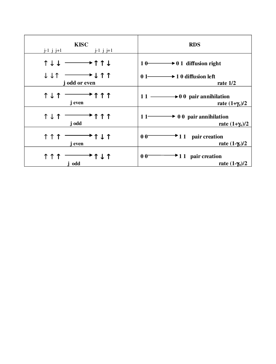
The KISC model is mapped onto an equivalent reaction-diffusion model with spatially alternating pair creation and annihilation rates in the following way. A dual lattice of $N$ sites is established, in which a site in the dual lattice is associted with the boundary between two sites in the KISC lattice. A pair of adjacent KISC spins with opposite signs is identified with a particle in the dual lattice; adjacent spins with the same sign is identified with the absence of a particle (a hole.) A spin flip in the KISC model translates into either diffusion of particles on the dual lattice with equal left-right rates, or pair creation or annihilation with different rates. Transition rates between configurations in the KISC system become diffusion, pair creation and annihilation rates in the RDS system, as shown in Table 1.

Time evolution of these systems is described by the master equation, expressing conservation of probability assuming a continuous-time dynamics. The probability $P(C,t)$ of finding the system in configuration $C$ at time $t$ increases due to transfer of probability into $C$ from other configurations, and decreases as $C$ passes probability into others, in such a way that $\sum_{C}P(C,t)=1$ for all $t$. The evolution of probability $P(C,t)$ is described by transition rates $r\left[C\rightarrow C^{\prime}\right]$, the probability per unit time that configuration $C$ changes into a different configuration $C^{\prime}$. The master equation is:

in which the first term on the right represents the gain in probability of configuration $C$ due to transitions from other configurations, and the second represents losses due to $C$ transforming into other configurations.

We utilize Dirac notation to represent each configuration as $|C\rangle$. From this we build a vector representation of a probabilistic superposition of all possible configurations of a system:

The master equation can now be re-expressed in terms of this vector as:

where the pseudo-Hamiltonian $H$ is a $2^{N}\times 2^{N}$ matrix, with matrix elements

A formal solution to Eq. 5 can be written as $|P(t)\rangle=e^{-Ht}|P(0)\rangle$. Our goal is to investigate the eigenvalues of operator $H$ in order to explain the system’s time dependence.

From this point, we shall focus on the RDS model. We follow the precedent of representing the “particles” and “holes” in the dual lattice by a spin one-half model: a particle is represented by spin up (and thus $|1\rangle$, a hole becomes a spin down ($|0\rangle$.) From the above formalism comes the definition of the probability-conserving operator $H$ that controls the system’s time dependence:

The operators $\sigma_{n}^{+}$ and $\sigma_{n}^{-}$ are the Pauli spin raising and lowering operators on the $n$-th cell:

It has been shown that the eigenvalues and eigenvectors of $H$ can be found if the “free fermion constraint” is obeyed [10]. For the RDS model, this means that the sum of local diffusion rates is equal to the sum of local pair creation and annihilation rates (in our case $\frac{1}{2}+\frac{1}{2}=\frac{1+\gamma_{o,e}}{2}+\frac{1-\gamma_{o,e}}{2}$.) This constraint assures the biliniarity of the $H$ operator, and, consequently, an exact solution for the problem.

Symmetries exhibited by the $H$ operator, Eq. 8, affect the form of its eigenvalues and eigenvectors, and in some cases aid in the process of determining them. In this section our goal is to exhibit these symmetries towards the goal of direct calculation of eigenvalues and eigenvectors of $H$ for small values of $N$.

Because the fundamental process described by the rate equation, Eq. 1, corresponds to the simultaneous flipping of two spins in the RDS model, the $H$ operator does not change the ’spin-parity’ of a state, i.e. states with an even number of up spins are transformed by $H$ into states of only even number of up spins, and likewise for odd numbers of up spins. This symmetry immediately separates the configuration space into two sub-spaces of the same dimensionality ($2^{N}/2$) which do not interact. Thus the $2^{N}\times 2^{N}$ $H$ matrix is reduced to two equal-sized diagonal blocks by proper ordering of the configuration basis states.

The $H$ matrix is also invariant to a translation of the ring of cells by an even number of cells to the right or left. Thus $H$ commutes with the operator that invokes this translation, and simultaneous eigenstates of the two operators can be found. Such eigenstates are conveniently written as sums of the form

($q=0,\ldots,N/2-1$), where $|C_{0}\rangle$ is a spin configuration (e.g. $|011000\rangle$ representing six spins, the second and third ones up, for the $1\times 6$ case) and $|C_{n}\rangle$ is the same configuration pushed $2n$ cells to the right using periodic boundary conditions (thus if $|C_{0}\rangle=|011000\rangle$, then $|C_{2}\rangle=|100001\rangle$.) The translation symmetry of the pseudo-Hamiltonian implies that $H$ does not mix states of the form $|\mathcal{C}_{q}\rangle$ which have different $q$ values. Thus within each of the two major sub-blocks of the $H$ matrix (one of even spin parity, one of odd spin parity) there are $N/2$ smaller sub-blocks, each with a different value of $q$. This symmetry has enabled relatively straightforward extraction of eigenvalues and eigenstates for even $N$ values up to $N=8$ (with a $256$-dimensional configuration space.)

Two additional symmetries are apparent from the form of $H$ given above, that provide further information regarding the form of the eigenvalues and eigenvectors.

The simultaneous translation of the spin chain by a single site (cell $n$ becomes cell $n+1$) along with the interchage of values $\gamma_{e}\leftrightarrow\gamma_{o}$ leaves $H$ invariant. If we use $\mathcal{X}$ to represent this transformation, it follows that $\mathcal{X}^{2}=I$. If $|\psi\rangle$ is an eigenstate of $H$ with eigenvalue $E$, then

This leads to several possibilities:

• •

  $E$ is invariant under the interchange $\gamma_{e}\leftrightarrow\gamma_{o}$ and either $\mathcal{X}|\psi\rangle$ is a constant multiple of $|\psi\rangle$, or $\mathcal{X}|\psi\rangle$ produces another eigenstate of $H$ distinct from $|\psi\rangle$ but with the same eigenvalue.

• •

  $E$ is not invariant under the interchange $\gamma_{e}\leftrightarrow\gamma_{o}$, but instead transforms to another distinct eigenvalue of $H$, and $\mathcal{X}|\psi\rangle$ becomes a corresponding eigenstate.

Explicit diagonalization for small $N$, shown in the next section, suggests that the eigenvalues are invariant under $\gamma_{e}\leftrightarrow\gamma_{o}$. The general solution for the eigenvalues presented in a later section show this to be true for all even values of $N$.

Another symmetry operation leaving $H$ invariant consists in changing the sign of both $\gamma$ constants and simultaneously flipping every spin. If we use $\mathcal{X}_{A}$ to represent this transformation, algebra similar to that of the prior paragraph leads to the following:

• •

  $E$ is invariant under the change in sign of both $\gamma$’s and either $\mathcal{X_{A}}|\psi\rangle$ is a constant multiple of $|\psi\rangle$, or $\mathcal{X_{A}}|\psi\rangle$ produces another eigenstate of $H$ distinct from $|\psi\rangle$ but with the same eigenvalue.

• •

  $E$ is not invariant under the change in sign of both $\gamma$’s, but instead transforms to another distinct eigenvalue of $H$, and $\mathcal{X_{A}}|\psi\rangle$ becomes a corresponding eigenstate.

Explicit diagonalization for small $N$ (following section) suggests also that the eigenvalues are invariant under the change in sign of both $\gamma$’s. This, too, is later proven true for all $N$.

The number of configurations for a given value of $N$, thus the dimensionality of the square matrix $H$, is $2^{N}$. This prohibits explicit diagonalization of $H$ for all but the smallest values of $N$. The symmetries of $H$ enable straightforward use of computer algebra software to find eigenvectors and eigenvalues for several cases. In this section some explicit results for $N=2,4,6,8$, so calculated, are exhibited and discussed.

Here we approach the problem using standard methodology [10]. Starting with the full, two-temperature operator in terms of spin raising and lowering operators, Eq. 8, we can rewrite in terms of fermionic operators ($c_{j}$, $c_{j}^{\dagger}$) that satisfy anti-commutation relations

This transformation, due to Jordan and Wigner [11] is as follows

Straightforward application of this transformation produces the ’fermionized’ pseudo-Hamiltonian

For the even spin-parity subspace the requirement that $\sigma^{+}_{N+1}=\sigma^{+}_{1}$ and $\sigma^{-}_{N+1}=\sigma^{-}_{1}$ implies $c_{N+1}=-c_{1}$ and $c^{\dagger}_{N+1}=-c^{\dagger}_{1}$. For the odd spin-parity case, $c_{N+1}=c_{1}$ and $c^{\dagger}_{N+1}=c^{\dagger}_{1}$. We take advantage of the translation symmetry mentioned in Section 3 by defining two kinds of fermions in momentum space, one created from even-numbered cells, the other from odd-numbered cells. Define the following momentum-space operators:

We chose q values to belong to the set $Q=\{\pm\frac{2\pi}{N},\pm\frac{6\pi}{N},\pm\frac{10\pi}{N},\ldots\pm\frac{(N-2)\pi}{N}\}$ for states with even spin-parity, and $Q=\{0,\pm\frac{4\pi}{N},\pm\frac{8\pi}{N},\ldots\pm\frac{(N-4)\pi}{N},\pi\}$ for states with odd spin-parity, to assure proper periodic boundary conditions for each case. These definitions of $Q$ assume that $N/4$ is integer-valued, but the ultimate results are valid as long as $N$ is even.

Like the operators $c_{j}$ and $c_{j}^{\dagger}$, the momentum space operators obey the canonical fermionic anticommutation relationships:

In terms of these operators, the pseudo-Hamiltonian is written as

The ultimate step in the derivation is to perform a Bogoliubov type similarity transform to new variables in which $H$ takes diagonal form. We postulate a diagonal form for $H$ that reads

while assuming that the operators $\chi_{q}$ and $\xi_{q}$ obey Fermionic anticommutation relations. Since $H$ is not Hermitian, $\tilde{\chi_{q}}\neq\chi_{q}^{\dagger}$, and $\tilde{\xi_{q}}\neq\xi_{q}^{\dagger}$. It is easily demonstrated that

Following Lieb, Schultz and Mattis[12] we define the $\chi_{q}$ and $\xi_{q}$ variables in terms of the $a_{q}$ and $b_{q}$ variables in the following manner:

and

where the $c_{i}$’s and $d_{i}$’s are constants. We can calculate the commutator with $H$ in the form given by Eq. 11 of each term in $\chi_{q}$ as expressed in Eq. 14, using

Constants in these expressions are defined as:

$\overline{\epsilon}$ represents $\epsilon$ as defined above but with $q$ replaced by $-q$, and likewise for $\epsilon^{\prime}$. Eq. 13, with these results used to evaluate the left hand side, produces a large operator equation. The coefficients of each of the four operators on the right-hand-side must equal the corresponding coefficient on the left-hand-side. This requirement produces a linear set of equations for the constants $c_{i}$ that can be expressed by the matrix equation $\omega_{q}C=MC$ where

and

Obviously, the eigenvalues of $M$ are possible values of the energies ($\omega_{q}$) of the $\chi$ excitations, which is what we seek. Identical analysis of the $d_{i}$ coefficients show that the eigenvalues of the same matrix are possible values of the energies ($\omega^{\prime}_{q}$) of the $\xi$ excitations. The eigenvector components are quite complicated, but the eigenvalues simplify easily. Two of the eigenvalue are negative, thus inappropriate candidates for the excitation energies (that we know to be positive.) The other two eigenvalues are $1\pm\cos{\frac{q}{2}}\sqrt{\gamma_{e}\gamma_{o}}$. Identify $\omega_{q}=1+\cos{\frac{q}{2}}\sqrt{\gamma_{e}\gamma_{o}}$ and $\omega^{\prime}_{q}=1-\cos{\frac{q}{2}}\sqrt{\gamma_{e}\gamma_{o}}$ in order to deduce the exact spectrum for the model.

There is a unique even spin-parity vacuum state $|0\rangle_{e}$ defined by the relations:

Other even spin-parity states are formed by an even number of excitations of the $\tilde{\chi}_{q}$ or $\tilde{\xi}_{q}$ type: each excitation of the former type carries energy $\omega_{q}$, and each of the latter type carries $\omega^{\prime}_{q}$. Since these excitations are fermionic, there cannot be two $\tilde{\chi}_{q}$ excitations with the same $q$, nor can there be two $\tilde{\xi}_{q}$ excitations with the same $q$. The highest energy state has $N/2$ distinct $\tilde{\chi}_{q}$ excitations and $N/2$ distinct $\tilde{\xi}_{q}$ excitations, and carries total energy $N$.

The odd spin-parity sector of the spectrum also has a unique vacuum:

References

- [1] Nonequilibrium statistical mechanics in one dimension, ed. V. Privman (Cambridge University Press, Cambridge, England, 1997.)
- [2] B. Schmittmann and R. K. P Zia, “Phase Transitions and Critical Phenomena” Vol 17, edited by C. Domb and J.L Lebowitz (Academic, London, 1995).
- [3] A. A. Lushnikov, Sov. Phys. JETP 64, 811 (1986); P.-A. Bares and M. Mobilia, Phys. Rev. E 59, 1996 (1999); Phys. Rev. Lett.: 83, 5214 (1999); S.-C. Park, J.-M. Park, and D. Kim, ibid. 85, 892 (2000); P.-A. Bares and M. Mobilia, ibid. 85, 893 (2000).
- [4] R. J. Glauber, J. Math. Phys. 4, 294 (1963).
- [5] F. Schmuser and B. Schmittmann, J. Phys. A: Math. Gen. 35, 2569 (2002);B. Schmittmann and F. Schmuser, Phys. Rev. E 66, 046130 (2002).
- [6] M. Henkel, E. Orlandini, and J. Santos Annals of Physics 259, 163 (1997).
- [7] N. Kuroda, Y. Wakabayashi, M. Nishida, N. Wakabayashi, M. Yamashita, and N. Matsushita, Phys. Rev. Lett. 79, 2510 (1997); N. Kuroda, M. Nishida, Y. Tabata, Y. Wakabayashi, K. Sasaki, Phys. Rev. B 61, 11217 (2000); Y. Tabata and N. Kuroda, Phys. Rev. B 61: 3085 (2000).
- [8] M. Mobilia, B. Schmittmann, and R. K. P. Zia, Phys Rev. E 71, 056129 (2005).
- [9] Z. Racz and R. K. P Zia, Phys Rev. E 49, 139 (1994).
- [10] M. D. Grynberg, T.J. Newman and R.B. Stinchcombe, Phys Rev. E 50, 957 (1994); M. D. Grynberg and R. B. Stinchcombe, Phys Rev. E 52, 6013 (1995).
- [11] P. Jordan and E. Wigner, Z. Phys. 47, 631 (1928).
- [12] E. Lieb, T. Schultz and D. Mattis, Ann. Phys. 16, 407 (1961).
- [13] G. L. Giorgi, Phys Rev. B 79, 060405(R) (2009).