Geometrical families of mechanically stable granular packings

Guo-Jie Gao¹ Affiliation: ¹ Department of Mechanical Engineering, Yale University, New Haven, CT 06520-8284.
² Department of Physics, Yale University, New Haven, CT 06520-8120. Jerzy Bławzdziewicz^1,2 Affiliation: ¹ Department of Mechanical Engineering, Yale University, New Haven, CT 06520-8284.
² Department of Physics, Yale University, New Haven, CT 06520-8120. Corey S. O’Hern^1,2 Affiliation: ¹ Department of Mechanical Engineering, Yale University, New Haven, CT 06520-8284.
² Department of Physics, Yale University, New Haven, CT 06520-8120.

August 24, 2026

Abstract

We enumerate and classify nearly all of the possible mechanically stable (MS) packings of bidipserse mixtures of frictionless disks in small sheared systems. We find that MS packings form continuous geometrical families, where each family is defined by its particular network of particle contacts. We also monitor the dynamics of MS packings along geometrical families by applying quasistatic simple shear strain at zero pressure. For small numbers of particles ( $N<16$ ), we find that the dynamics is deterministic and highly contracting. That is, if the system is initialized in a MS packing at a given shear strain, it will quickly lock into a periodic orbit at subsequent shear strain, and therefore sample only a very small fraction of the possible MS packings in steady state. In studies with $N>16$ , we observe an increase in the period and random splittings of the trajectories caused by bifurcations in configuration space. We argue that the ratio of the splitting and contraction rates in large systems will determine the distribution of MS-packing geometrical families visited in steady-state. This work is part of our long-term research program to develop a master-equation formalism to describe macroscopic slowly driven granular systems in terms of collections of small subsystems.

pacs

81.05.Rm, 83.80.Fg, 83.80.Iz

I Introduction

Dry granular materials are collections of discrete, macroscopic particles that interact via dissipative and purely repulsive interactions, which are nonzero when particles are in contact and vanish otherwise. Granular systems range from model systems composed of glass beads to pharmaceutical powders, to soils and geological materials.

A distinguishing feature of granular materials is that they are athermal. Since individual grains are large, thermal energy at room temperature $T$ is unable to displace individual grains. Thus, without external driving, granular materials are static and remain trapped in a single mechanically stable (MS) grain packing with force and torque balance on each grain. In contrast, when external forces are applied to granular materials, these systems flow, which gives rise to grain rearrangements, fluctuations in physical quantities like shear stress and pressure, and the ability to explore configuration space.

There are many driving mechanisms that generate dense flows in granular media—for example, oscillatory [1, 2, 3, 4] and continuous shear [5, 6], horizontal [7] and vertical vibration [8, 9], and gravity-driven flows [10]. The fact that driven granular systems can achieve steady-states, explore configuration space, and experience fluctuations as in thermal systems, has prompted a number of groups to describe these flows using concepts borrowed from equilibrium statistical mechanics (such as effective temperature) [11, 12, 13, 14, 15, 16].

However, before a statistical mechanical treatment can be rigorously applied to dense granular flows, fundamental questions about the nature of configuration space should be addressed. In particular, one needs to determine how dense granular systems sample configuration space: Is it uniformly sampled or are some states visited much more frequently than others? How is the sampling of configuration space affected by the strength and type of driving and dissipation mechanisms? In this work and a series of recent papers [18, 17, 19, 20], we address these questions with the goal of developing a comprehensive physical picture for static and slowly driven granular matter.

In our previous studies, we focused on the statistical properties of static frictionless disk packings generated by slow compression without gravity [18, 17, 19] or by gravitational deposition [20]. We have determined that the probability distribution for mechanically stable packings is strongly peaked around the value typically quoted for the random-close packing (RCP) volume fraction, and explained why RCP is obtained by many compaction protocols. We have also found that the MS-packing probabilities are highly non-uniform, contrary to the Edwards’ equal-probability assumption [21] that is frequently used in thermodynamic descriptions of granular matter [14]. In addition, we have found that the probabilities become more non-uniform with increasing system size [17].

In the present article, we further explore the statistics of granular microstates and its relevance for static and dynamic properties of granular materials. We focus on slowly sheared systems at fixed zero pressure, where the evolution can be approximated as a sequence of transitions between MS packings. One of our novel results is that slowly sheared MS packings occur as continuous geometrical families defined by the network of particle contacts. Moreover, these geometrical families are not uniformly sampled during quasistatic shear flow. We focus on small systems, so that we are able enumerate nearly all MS packings and obtain accurate packing probabilities as a function of shear strain. Since our results indicate the need for developing an alternative approach to the quasi-thermodynamic descriptions based on the Edwards’ ideas, we advocate here a new master-equation framework for understanding dense granular flows.

This paper is organized as follows. In Sec. II, we provide motivation for our investigations by introducing a simple phenomenological master-equation model that reproduces qualitatively some of the key features of slowly-driven granular systems. In Secs. III and IV, we introduce our model system, 2D bidisperse mixtures of frictionless, purely repulsive, soft grains, and describe the simulation method that we employ to generate mechanically stable packings. Here, we also clearly define the set of distinct mechanically stable (MS) packings in terms of the eigenvalues of the dynamical matrix and discuss their symmetries. In Sec. V, we outline our method to study quasistatic simple shear flow of frictionless disks in small 2D systems at zero pressure. In Secs. VI, we describe the results of the quasistatic shear simulations, with a particular emphasis on enumerating geometrical families of MS packings and determining how they are sampled during quasistatic dynamics. In Sec. VII provide an outlook for further work on larger system sizes. The main conclusions of our studies and their relation to our long-term research program are discussed in Sec. VIII. In Appendices A, B, and C, we provide details of the numerical simulations, the calculation of the dynamical matrix for the repulsive linear spring potential used in these studies, and the method used to distinguish ‘polarizations’ of MS packings (i.e., MS packings that differ only by reflection or rotation).

II Motivation

Refer to caption — Figure 1: (a) Packing density $\rho$ for mm glass beads as a function of tapping intensity $\Gamma$ (normalized by $g$ ). The system is initialized in a dilute state at $\rho=0.59$ and then subjected to vibrations of increasing intensity. At each $\Gamma$ , the system is tapped until it achieves a steady-state $\rho$ . After reaching $\Gamma=7$ , the tapping intensity is decreased until $\Gamma<1$ , and then increased again. Data is reprinted from Ref. [8]. Copyright 1998, The American Physical Society. (b) Packing fraction $\phi$ for mm glass beads as a function of shear angle $\theta$ during cyclic shear. $\theta$ is increased linearly in time from $2.7^{\circ}$ to $10.7^{\circ}$ , then decreased to $2.7^{\circ}$ , and finally increased again to $10.7^{\circ}$ . Data is reprinted from Ref. [5]. Copyright 2000, Springer-Verlag.

Granular materials are athermal—they are unable to thermally fluctuate and sample phase space. However, if a grain packing is perturbed by external forces, it can move through a series of configurations. The set of states populated by a granular system during a series of discrete vertical taps was characterized in Ref. [8]. As shown in Fig. 1(a), an initially loose packing is compacted by tapping first gently, and then with greater intensity. At sufficiently large tapping intensities, it is no longer possible to further compact the system. However, when the tapping intensity is reduced, the packing fraction increases, rather than returning along the original packing fraction trajectory. This new curve (packing fraction vs. tapping intensity) obtained by successively decreasing and then increasing the tapping intensity in small steps is nearly reversible. A similar phenomenon has been found in granular media undergoing cyclic shear [5], as shown in Fig. 1(b).

These experiments, which show that slowly driven granular systems appear to explore a well-defined set of states reversibly, have prompted a number of theoretical studies aimed at describing compacting granular systems using quasi-thermodynamic approaches based on the Edwards’ ensemble (i.e. the assumption of equally probable microstates) [22, 23, 26, 25, 24]. However, in previous work [18, 17, 19, 20], we have shown explicitly for small systems that the probability distribution for mechanically stable packings is highly non-uniform. Moreover, we have demonstrated that this feature is not sensitive to the packing-generation protocol and becomes more pronounced as the system size increases. Thus, we argue that the Edwards’ equal-probability assumption is not valid and alternate theoretical approaches for slowly driven granular systems must be developed.

Although several alternatives have been put forward [16, 27, 28], we advocate here for a master-equation approach for the following reasons. First, quasistatic evolution of slowly driven granular systems can be approximated as a sequence of transitions between MS packings. Second, since the system undergoes particle rearrangements as it transitions between MS packings, it retains little memory from one MS packing to the next, and successive MS packings are nearly statistically independent. Thus, slowly driven granular systems can be approximated as a Markov chain of independent transitions between MS packings and described using a master-equation approach.

We have shown that the form of the microstate probability distribution can be qualitatively reproduced by combining probabilities for small subsystems. Thus, we also advocate a novel ‘bottom-up’ approach in which large granular systems are described as collections of nearly independent subsystems. We view this work on small quasistatically sheared MS packings as laying the groundwork for future studies that will apply the master-equation approach to quantitatively describe the statistical properties of dense granular flows.

II.1 Model

To illustrate the importance of the above-mentioned features in capturing the irreversible and reversible branches in Fig. 1, we construct a simple model in which a granular system is represented as a collection of ${\overline{N}}$ statistically independent small subdomains. Each subdomain $j=1,\ldots,{\overline{N}}$ can reside in one of several microstates $k_{j}=1,\ldots,m$ . The volume of the subdomain $j$ in state $k_{j}$ is $V_{1}(j,k_{j})$ , and these subvolumes are assumed to be additive

V(\Lambda)=\sum_{j=1}^{\overline{N}}V_{1}(j,k_{j}),

(1)

where $V(\Lambda)$ is the volume of the whole system in the state $\Lambda=(k_{1},\ldots,k_{\overline{N}})$ . Since the subdomains are assumed to be statistically independent, the joint probability distribution for the whole system is

P(\Lambda;t)=\prod_{j=1}^{\overline{N}}P_{j}(k_{j};t),

(2)

where $P_{j}(k_{j};t)$ is the probability distribution for the microstates of subdomain $j$ at time $t$ .

The evolution of subdomains in a system driven by an applied force of strength $\lambda$ is described by ${\overline{N}}$ independent master equations

	$\displaystyle P_{j}(k;t_{i+1})=P_{j}(k;t_{i})+\sum_{k^{\prime}=1}^{m}[W_{kk^{\prime}}(\lambda)P_{j}(k^{\prime};t_{i})-$
	$\displaystyle W_{k^{\prime}k}(\lambda)P_{j}(k;t_{i})],$		(3)

where $W_{kk^{\prime}}$ is the transition probability from state $k^{\prime}$ to state $k$ .

To qualitatively reproduce the irreversible and reversible branches of states when the magnitude of the external forcing $\lambda$ is ramped up and down, we use simple assumptions regarding the volume distribution of individual subsystems and the transition probabilities. We assume that the volumes of individual subsystems are given by the expression

V_{1}=r(V_{0}+A\mathrm{e}^{-\kappa_{v}x_{i}}),

(4)

where $V_{0}$ , $A$ , and $\kappa_{v}$ are constants, $x_{i}=(i-1)/(k-1)$ , and $r$ is a random number. Note that states with higher indexes possess smaller volumes. The transition rates are modeled by the expression

W_{ij}=Cb(x_{ij})r_{w}\textrm{e}^{-[x_{ij}/\sigma_{0}\lambda(t)]^{2}},

(5)

where $C$ is the normalization constant, $b(x_{ij})$ is a bias function

b(x)=\left\{\begin{array}[]{ll}b_{\textrm{min}}+b_{0}(1-2\lambda)&\qquad x>0,\\ 1&\qquad x<0\end{array}\right.

(6)

with constants $b_{\rm min}$ and $b_{0}$ , which introduces asymmetry between up and down jumps, $\sigma_{0}$ determines the width of the Gaussian distribution, and $r_{w}$ is a random number. As shown in Fig. 2, such a simple master-equation approach is able to qualitatively reproduce features (evolution of the system to a reversible branch of the packing fraction) found in vertical tapping and cyclic shear studies of granular materials. The success of this simple model emphasizes two key points: 1. Only minimal constraints on transition probabilities are required (not thermodynamics) to reach steady-state and 2. An assumption of weakly interacting small subsystems may be able to explain macroscopic phenomena in slowly driven granular media.

These results suggest a new approach to describe the quasistatic evolution of granular systems: a Markov process characterized by transfer rates between MS packing microstates. To further develop this approach so that it can yield quantitative predictions, one must determine (a) the types of microstates that occur in static granular systems and (b) transition probabilities between these microstates when the system is slowly driven. To provide the necessary input for constructing quantitative descriptions, in this paper we study the structure of configuration space and transitions between microstates in small 2D granular systems undergoing quasistatic shear strain at fixed zero pressure.

III Small periodic granular packings in simple shear

III.1 Bidisperse frictionless disks

We consider 2D systems of soft, frictionless disks interacting via the pairwise additive purely repulsive linear spring potential

V({\vec{\xi}})=\sum_{i<j=1}^{N}V_{2}(r_{ij}),

(7)

V_{2}(r_{ij})=\frac{\epsilon}{\alpha}\left(1-r_{ij}/\sigma_{ij}\right)^{\alpha}\Theta\left(\sigma_{ij}/r_{ij}-1\right),

(8)

where $\alpha=2$ , $\vec{\xi}=(\vec{r}_{1},\ldots,\vec{r}_{N}$ ) denotes the system configuration, $\vec{r}_{i}$ is the position of the center of disk $i$ , $r_{ij}=|\vec{r}_{i}-\vec{r}_{j}|$ is the center-to-center separation between disks $i$ and $j$ , and the sum is over distinct particle pairs. The strength of the spring potential (8) is characterized by the energy scale $\epsilon$ , and the range by the average particle diameter $\sigma_{ij}=\left(\sigma_{i}+\sigma_{j}\right)/2$ . The Heaviside step function $\Theta(x)$ turns off the interaction potential when the particle separation is larger than $\sigma_{ij}$ .

All numerical simulations described in this paper were performed for 50-50 (by number) binary mixtures of large and small particles with diameter ratio $1.4$ . In such bidisperse mixtures, shear-induced crystallization is inhibited [29]; thus the system is well suited for investigations of quasistatic evolution of disordered granular systems. We focused on small systems with the number of particles in the range $N=4$ to $20$ .

To mimic the behavior of granular packings, we consider MS disk configurations at infinitesimal pressure and particle overlaps. As shown in our recent experimental and numerical study, statistical properties of disks interacting via the repulsive linear spring potential (8) closely match properties of plastic and steel disks in a system where frictional forces have been relaxed using high-frequency, low-amplitude vibrations [20].

III.2 Shear-periodic boundary conditions

In our simulation studies, the particles are confined to a $L\times L$ periodic box, as illustrated in Fig. 3. The unit cell can either be a square [cf. Fig. 3(a)], or it can be deformed in the $x$ direction [cf., Figs. 3(b) and (c)]. These shear-periodic boundary conditions allow us to generate an ensemble of anisotropic granular packings as a function of the shear strain $\gamma=\Delta x/L$ , where $\Delta x$ is the horizontal shift of the top image cells relative to the bottom image cells. Moreover, simulations of systems with gradually changing strain [30, 31] enable us to study quasistatic evolution of a granular packing under shear.

Note that shear-periodic boundary conditions are identical at $\gamma$ and $1-\gamma$ as shown in Fig. 3. Also, when reflection symmetry is taken into account, it is clear that we only need to consider shear strains in the range $\gamma=[0,0.5]$ to generate static packings at arbitrary shear strains. However, in the case of continuous quasistatic shear flow, evolution of the system over multiple shear strain units must be investigated to capture the full dynamics.

Table 1: Number of distinct MS packings at integer shear strains when we treat all polarizations as the same

N_{s}

and when we distinguish among different polarizations

N_{s}^{p}

as a function of system size

N

. The third column gives the ratio

N_{s}^{p}/N_{s}

. Data for

N_{s}

is obtained from Ref. [17].

$N$	$N_{s}$	$N_{s}^{p}$	$N_{s}^{p}/N_{s}$
$4$	$3$	$6$	$2.00$
$6$	$20$	$68$	$3.40$
$8$	$165$	$612$	$3.71$
$10$	$1618$	$6378$	$3.94$
$12$	$23460$	$91860$	$3.92$

IV Enumeration of MS packings at arbitrary shear strain

IV.1 Packing-generation protocol

Zero-pressure MS packings at a given shear strain are generated using the compression/decompression packing-generation protocol used in our previous studies of unsheared MS packings [17]. We briefly outline the procedure below for completeness. We begin the packing-generation process by choosing random initial particle positions within the simulation cell at packing fraction $\phi_{0}=0.50$ (which is well below the minimum packing fraction at which frictionless MS packings occur in 2D). We then successively increase or decrease the diameters of the grains, with each compression or decompression step followed by conjugate gradient minimization [32] of the total energy in (7).

As illustrated in Fig. 4, the system is decompressed when the total energy (7) at a local minimum is nonzero—i.e., there are finite particle overlaps [cf., Figs. 4 (a) and (d)]. If the potential energy of the system is zero [Fig. 4(c)] and gaps exist between particles [Fig. 4(f)], the system is compressed. The increment by which the packing fraction $\phi$ is changed at each compression or decompression step is gradually decreased. Numerical details of the algorithm are provided in Appendix A.

In the final state of the packing-generation process, the potential energy vanishes [Fig. 4(b)], but any change of the relative particle positions (excluding rattler particles, which can be moved without causing particle overlap) results in an increase in the potential energy. Thus, the final state is a mechanically stable configuration (or collectively jammed state [33]) at jamming packing fraction $\phi_{J}$ . At each fixed $\gamma$ , MS packings form a discrete set in configuration space. The packing-generation process is repeated more than $10^{6}$ times for at least $100$ uniformly spaced shear strain values in the interval $0<\gamma<0.5$ . A large number of independent trials is required to enumerate nearly all MS packings because the MS probability distribution varies by many orders of magnitude.

IV.2 Classification of granular packings

IV.2.1 Dynamical matrix

With our precise measurement of the jamming packing fraction $\phi_{J}$ to within $10^{-8}$ of the jamming point, it is very rare that two distinct MS packings have the same $\phi_{J}$ . Thus, it is often convenient to characterize MS packings by $\phi_{J}$ . However, in our detailed investigations of the quasistatic evolution of sheared granular packings, a more precise classification of MS packings is necessary.

To determine the set of distinct MS packings, we use the eigenvalues and eigenvectors of the dynamical matrix [34]

{\bf M}_{mn}=\left.\frac{\partial V}{\partial{\xi}_{m}\partial{\xi}_{n}}\right|_{{\vec{\xi}}_{0}},

(9)

where $\xi_{m}$ is the $m$ th component of the configuration vector $\vec{\xi}$ and ${\vec{\xi}}_{0}$ gives the configuration of the reference MS packing. Since rattler particles do not contribute to the stability of the system, we consider only the dynamical matrix for the mechanical backbone of the packing. This matrix has $d{\cal N}$ rows and columns, where $d=2$ is the spatial dimension, ${\cal N}=N-N_{r}$ is the number of particles in the mechanical backbone, and $N_{r}$ is the number of rattler particles.

Since the dynamical matrix is symmetric, it has $d{\cal N}$ real eigenvalues $\{m_{i}\}$ , $d$ of which are zero due to translational invariance of the system. In a mechanically stable disk packing, no collective particle displacements are possible without creating an overlapping configuration; therefore the dynamical matrix for MS packings has exactly $d({\cal N}-1)$ positive eigenvalues [35]. We limit the results below to mechanically stable packings.

IV.2.2 Polarizations

According to our previous investigations [17, 18], distinct MS packings always have distinct sets of eigenvalues $\{m_{i}\}$ , except when packings can be related to each other by reflection or rotation [35]. When we treat different ‘polarizations’ associated with each symmetry transformation as the same state, distinct MS packings can be classified according to the lists of eigenvalues of their dynamical matrices. This approach was adopted in Refs. [17, 18], where we considered only static, isotropic particle configurations at $\gamma=0$ . The eight equivalent polarizations for a MS packing at $\gamma=0$ are shown in Fig. 5.

In contrast, in our present study we consider continuous shear deformations of the system. After an isotropic unit cell is deformed, different polarizations of a given state can be transformed into distinct MS packings (i.e., packings distinguishable by the lists of eigenvalues $\{m_{i}\}$ ). For example, all polarizations shown in the left (right) column of Fig. 5, after a step strain are transformed into non-equivalent configurations. Our present classification scheme for MS packings takes this effect into account.

Accordingly, we treat states that differ by reflection or rotation by the angle $\alpha=\pi/2$ or $3\pi/2$ as distinct MS packings. However, due to symmetry of shear flow (cf. bottom of Fig. 5), the states that are related by a rotation by the angle $\alpha=\pi$ deform in equivalent way. Therefore, such states are treated as equivalent states. Further details regarding polarizations of MS packings, including the procedure we use to distinguish polarizations, are discussed in Appendix C.

IV.3 Distinct MS packings at integer and non-integer strains

MS packings at integer shear strains have equivalent boundary conditions to those in standard square periodic cells (as shown in Fig. 3). Thus, we can use our previous extensive calculations of MS packings generated in square cells with periodic boundary conditions [17].

In Table 1 we show the number of distinct MS packings at integer shear strains $N_{s}$ when we treat all polarizations as the same (data from Ref. [17]) and $N_{s}^{p}$ when we account for different polarizations (as described above). The ratio $N_{s}^{p}/N_{s}$ is smaller than $4$ because of reflection or rotation symmetry of some MS packings. As depicted in Fig. 6, both $N_{s}$ and $N_{s}^{p}$ grow exponentially with system size.

The number of distinct MS packings $N_{s}^{p}(\gamma)$ (including polarizations) versus shear strain is shown in Fig. 7 for several system sizes. The results show that (1) the maximum number of distinct packings occurs at integer and half-integer shear strains, and (2) there is a noticeable dip in $N_{s}^{p}$ at $\gamma^{*}\approx 0.2$ . However, as the system size increases, the number of distinct MS packings becomes uniform as a function of shear strain.

Table 2: The maximum transient shear strain

\gamma_{t}^{\rm max}

and period

T

of each distinct periodic orbit in integer strain units for several system sizes

N

. (

\gamma_{t}^{\rm max}

is rounded to the nearest integer shear strain.) In the fourth column, we list the average jammed packing fraction

\langle\phi_{J}\rangle

of the MS packings that are dynamically accessible at large shear strain for each each periodic orbit. For systems with multiple periodic orbits, we list

\gamma^{\rm max}_{t}

T

, and

\langle\phi_{J}\rangle

for each.

$N$	$\gamma^{\rm max}_{t}$	$T$	$\langle\phi_{J}\rangle$
$4$	$2$	$1$	$0.829$
$6$	$2$	$1$	$0.777$
$8$	$5$	$1$	$0.820$
	$1$	$2$	$0.825$
$10$	$1$	$1$	$0.815$
	$3$	$1$	$0.808$
	$4$	$1$	$0.833$
	$2$	$2$	$0.812$
$12$	$1$	$1$	$0.782$
	$12$	$3$	$0.815$
$14$	$0$	$1$	$0.811$
	$1$	$1$	$0.789$
	$2$	$1$	$0.814$
	$2$	$1$	$0.816$
	$2$	$1$	$0.814$
	$3$	$1$	$0.847$
	$3$	$1$	$0.815$
	$4$	$1$	$0.847$
	$36$	$1$	$0.836$
	$8$	$5$	$0.804$

Table 3: Catalog of the

N_{s}^{p}=68

possible transitions from a MS packing with index

i

\gamma=0

to index

j

\gamma=1

for quasistatic shear flow at zero pressure for

N=6

$i(\gamma=0)$	$j(\gamma=1)$	$i(\gamma=0)$	$j(\gamma=1)$	$i(\gamma=0)$	$j(\gamma=1)$
$1$	$37$	$26$	$67$	$51$	$62$
$2$	$67$	$27$	$37$	$52$	$67$
$3$	$37$	$28$	$62$	$53$	$67$
$4$	$62$	$29$	$67$	$54$	$67$
$5$	$67$	$30$	$62$	$55$	$67$
$6$	$62$	$31$	$62$	$56$	$67$
$7$	$67$	$32$	$67$	$57$	$67$
$8$	$67$	$33$	$62$	$58$	$67$
$9$	$62$	$34$	$37$	$59$	$67$
$10$	$37$	$35$	$67$	$60$	$67$
$11$	$67$	$36$	$62$	$61$	$67$
$12$	$67$	$37$	$67$	$62$	$67$
$13$	$67$	$38$	$62$	$63$	$67$
$14$	$67$	$39$	$37$	$64$	$62$
$15$	$67$	$40$	$67$	$65$	$67$
$16$	$62$	$41$	$37$	$66$	$67$
$17$	$62$	$42$	$67$	$67$	$67$
$18$	$67$	$43$	$67$	$68$	$67$
$19$	$62$	$44$	$62$
$20$	$37$	$45$	$67$
$21$	$62$	$46$	$37$
$22$	$67$	$47$	$67$
$23$	$67$	$48$	$67$
$24$	$67$	$49$	$67$
$25$	$37$	$50$	$37$

V Quasistatic shear flow at zero pressure

V.1 System dynamics

V.1.1 Quasistatic shear-strain steps

To mimic quasistatic evolution of a frictionless granular packing, we apply a sequence of successive shear-strain steps of size $\delta\gamma\ll 1$ to a system of bidisperse disks with shear-periodic boundary conditions. Each step of the protocol consists of (1) shifting the $x$ -coordinate of the particles,

x_{i}\rightarrow x_{i}+\delta\gamma y_{i},

(10)

in conjunction with the corresponding deformation of the unit cell; and (2) the compression/decompression packing-generation process (described in Sec. IV.1) to achieve a zero-pressure MS configuration with infinitesimal particle overlaps.

This procedure generates quasistatic shear flow at constant zero pressure (but varying packing fraction), which is an appropriate description of slowly sheared granular matter, where particle overlaps are always minimal. During the evolution, the system constantly expands and contracts to remain at the onset of jamming with packing fraction $\phi_{J}$ that depends on $\gamma$ . We note that our procedure is distinct from the quasistatic evolution used in recent investigations of sheared glass-forming liquids [37, 36], where a constant-volume ensemble was implemented.

V.1.2 Particle rearrangements

During a single shear-strain step $\delta\gamma$ , particle positions can either change continuously or a sudden particle rearrangement can occur. A continuous evolution step is schematically depicted in the left panels of Fig. 8, and the right panels illustrate a strain step that yields a particle rearrangement.

In both cases, the system initially resides in the local minimum (point $1$ ) in the energy landscape. Since this minimum corresponds to a MS packing, its energy is infinitesimal. When the affine transformation (10) is applied, the system moves to point $2$ in the energy landscape. In the case of continuous evolution, depicted in Fig. 8(a), the energy minimization (point $3$ ) and subsequent decompression (point $4$ ) move the system back to the neighborhood of the initial packing. As illustrated in 8 (c), at the initial and final points ( $1$ ) and ( $4$ ), the topology of contact networks is unchanged.

In contrast, when the energy minimization that follows an affine shear-strain step drives the system into a zero-energy region corresponding to an unjammed packing (i.e. point $3$ in Fig. 8(b)), upon subsequent compaction the system is driven to a MS packing (point $4$ ) with a different contact network than the initial packing (point $1$ ), as illustrated in Fig. 8(d).

During the continuous portion of the quasistatic shear strain evolution, the MS packings that are visited do not depend on the energy minimization method (e.g., energy relaxation via dissipative forces versus the conjugate gradient algorithm [17]) or parameters related to the compaction and decompression processes. Dynamical features do not influence the MS packings that are obtained along the continuous region because the system remains in the basin of the original mechanically stable packing. However, when a shear strain step leads to particle rearrangements, the system is taken to a new region of the energy landscape, and the energy minimization scheme, compaction and decompression rates, and even the location of rattler particles can influence the final MS packing. In small systems ( $N<16$ ), we find that the dynamics is weakly sensitive to these features, whereas in larger systems noise and protocol dependence play an important role in determining steady-state MS packing probabilities. In Sec. VII, we will describe future work in which we will tune the dynamics to determine its influence on the transition rates among MS packings.

V.2 Deterministic and contracting evolution of small frictionless MS packings

Our key results regarding quasistatic evolution of small granular systems are summarized in Figs. 9 and 10 and in Tables 2 and 3. The results show that (1) the evolution of small systems is deterministic; (2) after transient evolution, the system becomes locked into a periodic orbit; and (3) the evolution in configuration space is strongly contracting, in the sense that each unit strain leads to a significant reduction of the number of dynamically accessible MS packings.

Deterministic evolution

The deterministic character of the system evolution over continuous portions of the trajectories can be justified using arguments based on the continuity of the energy landscape, similar to those illustrated in Fig. 8 (a). The exceptions are bifurcation points, which will be described in Sec. VII. Indeterminacy can also occur due to the presence of rattlers or random particle motions in unjammed configurations. For systems with $N<16$ evolved according to the algorithm described in Sec. V.1.1, the observed evolution was always completely deterministic. Random evolution in larger systems and systems with random noise are discussed in Sec. VII.

Periodic orbits

In Fig. 9, we track the evolution of the jammed packing fraction $\phi_{J}$ as a function of shear strain $\gamma$ during zero-pressure quasistatic shear flow after the system is initialized in one of the MS packings at $\gamma=0$ for $N=10$ particles. Fig. 9 shows the complete trajectory and the inset shows $\phi_{J}$ only at integer strains. We observe that after a short transient of approximately two units of strain, the system becomes locked into a periodic orbit (with unit period $T=1$ ). Similar behavior is observed for systems with $N=4$ to $14$ particles, as summarized in Table 2. Although we have a limited range of system sizes for which a complete analysis of the quasistatic evolution has been preformed, the results show that both the transient time $\gamma_{t}$ and period $T$ increase somewhat with system size. (Note that several periodic orbits for $N=12$ and $14$ particles have anomalously large transients, cf. Sec. VII.)

Contracting evolution

The contracting character of the quasistatic shear flow is illustrated in the ‘tree’ diagram in Fig. 10. This digram represents the complete set of trajectories, shown for integer strain, for a system of $N=6$ particles. For this system size there are $N_{s}^{p}=68$ possible MS packings at any given integer shear strain, yet only one of them is dynamically accessible in the large shear strain limit.

The contraction of the set of dynamically accessible states as the system evolves results from the deterministic and irreversible character of quasistatic evolution. As illustrated in Fig. 10, from each MS packing at an integer strain $\gamma$ , the system transitions to a unique MS packing at the strain $\gamma+1$ ; however, more than one state can transition to a given state. A complete catalog of transitions at integer shear strains for the system of $N=6$ particles is given in Table 3. From this table, a complete list of trajectories of the whole evolution process can be constructed without further simulations.

As shown in Table 2, the number of periodic orbits to which the system contracts increases with the system size. However, for all systems studied, the number of orbits and the number of states visited at long times is small compared to the total number of MS packings.

The results in the last column of Table 2 give the average jammed packing fraction $\langle\phi_{J}\rangle$ of the MS packings sampled for a given periodic orbit. The MS packings that occur in periodic orbits typically have the highest packing fractions out of the entire distribution.

VI Family structure of the set of MS packings

An analysis of the deterministic evolution of the system monitored at integer values of strain is sufficient to conclude that the dynamics is contracting and periodic at large shear strains. However, it might be puzzling that both the transient shear strain and period are so short, i.e., much shorter than the number of MS packings (cf., Tables 1 and 2). To shed light on this behavior we will now analyze how the sets of MS packings at different values of shear strain are connected.

VI.1 Construction of continuous geometrical families of MS packings

As described in Sec. IV.2, we can identify the distinct MS packings at a given shear strain using the eigenvalues of the dynamical matrix. However, this method will not work for comparing MS packings at different shear strains since the eigenvalues vary continuously with $\gamma$ .

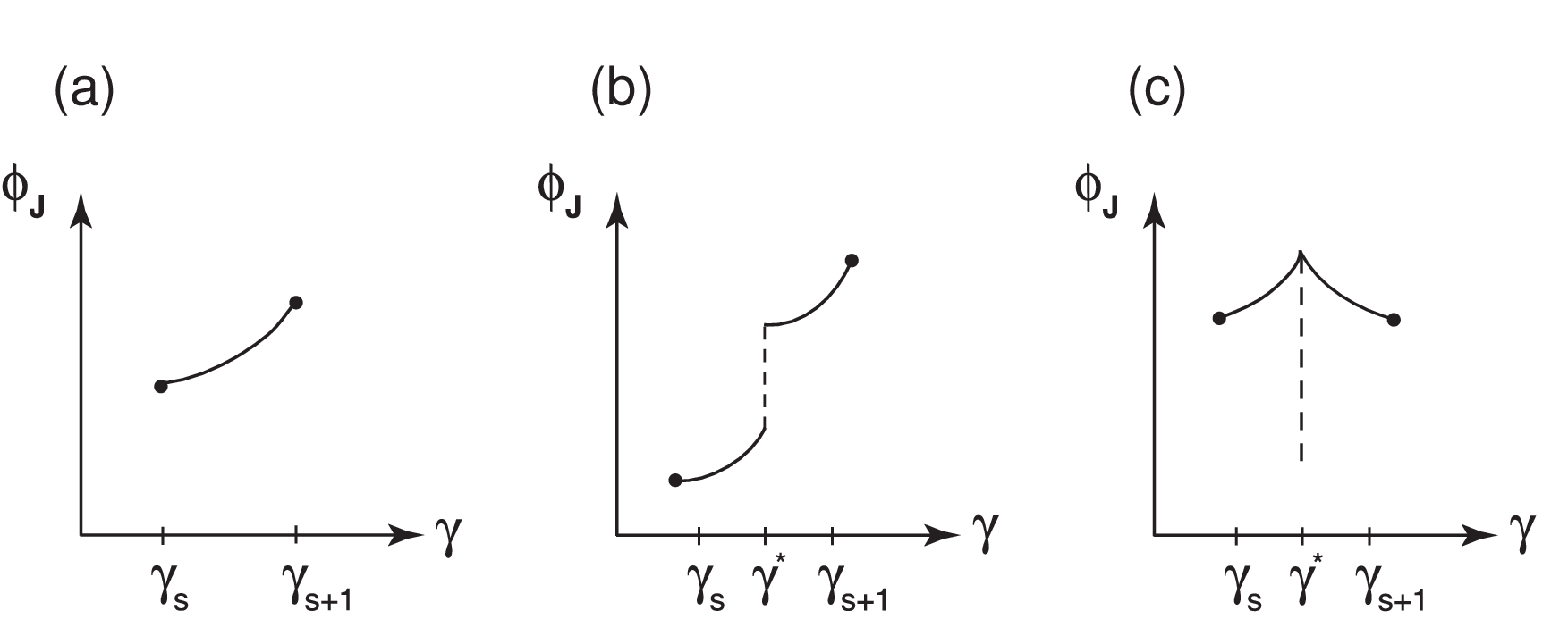
To study the relationship between distinct MS packings at different shear strains, we divide the shear strain region into small intervals $\gamma_{s+1}-\gamma_{s}$ . For each distinct MS packing at $\gamma_{s}$ , we monitor the particle contact network as the system evolves toward $\gamma_{s+1}$ (and $\gamma_{s-1}$ ). In Fig. 11 (a), we show the continuous evolution of $\phi_{J}$ between $\gamma_{s}$ and $\gamma_{s+1}$ , which implies that there are no rearrangement events and no changes in the particle contact network during this interval. Thus, the continuous evolution of $\phi_{J}$ identifies a portion of a geometrical family of MS packings all with the same particle contact network that exist over a continuous shear strain interval.

In our simulations, we find that changes in the network of particle contacts (i.e. switches from one geometrical family to another) is accomplished either by jumps (discontinuities in $\phi_{J}$ ) or kinks (discontinuities in the derivative of $\phi_{J}$ with respect to $\gamma$ ) as shown in Figs. 11 (b) and (c), respectively. As will be discussed in Sec. VI.2, a discontinuity in $\phi_{J}$ corresponds to a system instability and a change in the contact network with finite particle displacements; whereas a discontinuity in the derivative of $\phi_{J}$ corresponds to a change of the contact network without finite particle displacements.

To construct the complete map of distinct geometrical families for all shear strain, we can simply link the equivalent geometrical families at the shear strain endpoints $\gamma_{s}$ , or terminate the family if it has no counterpart. Because of the contracting dynamics described in Sec. V.2, it is important to use sufficiently small shear strain intervals so that we have enough shear strain resolution to capture small families. (See Appendix A for additional details for constructing geometrical families.)

Table 4: Statistics for complete geometrical family maps. Total number of distinct geometrical families

N_{f}

, average number of distinct MS packings

\langle N_{s}^{p}(\gamma)\rangle

, average packing fraction

\langle\phi_{J}(\gamma)\rangle

, average family length

\xi

, and average family second derivative

{\cal C}

for several system sizes

N

[38].

$N$	$N_{f}$	$\langle N_{s}^{p}(\gamma)\rangle$	$\langle\phi_{J}(\gamma)\rangle$	$\xi$	${\cal C}$
$4$	$15$	$4$	$0.788$	$0.18$	1.7
$6$	$334$	$47$	$0.739$	$0.06$	5.6
$10$	$34822$	$2896$	$0.753$	$0.03$	4.9

VI.2 Complete map of MS packings for continuous shear strain

We find that a particularly simple, pictorial method to distinguish geometrical families is by monitoring the jamming packing fraction $\phi_{J}$ as a function of shear strain (instead of a complete representation of the particle contact network). The complete map of MS packings— $\phi_{J}$ for all distinct MS packings at all shear strains—is displayed in Fig. 12 for $N=6$ . The structure of the map is quite complex even for $N=6$ , and it possesses a number of distinctive features.

First, the map is composed of a finite number ( $N_{f}=334$ for $N=6$ ) of curved concave-up segments each of which corresponds to a distinct geometrical family of MS packings. Second, the parabola-like curves either end discontinuously [cf., point 2 in the blowup shown in Fig. 12 (b)] or form a kink [points 4 and 5 in Fig. 12 (b)]. Third, the curves significantly vary in length, and they are not symmetric about the apexes (which are distributed over the full range of $\gamma$ [39]).

We find that a given parabola-like curve ends when either the contact network of that particular continuous region becomes unstable and the system jumps to a new one or the contact network merges with another network to form a kink. Examples of contact networks corresponding to characteristic points on the family map are shown in Fig. 12 (c).

Figure 13 shows that the family-length distribution is exponential (with the characteristic strain of $\xi\sim 0.06$ for N=6 [40]) and the distribution of second derivatives possesses a strong peak. We speculate that the decay length $\xi$ is related to the average yield strain in frictionless MS packings. Thus, it is important to study $\xi$ as a function of system size and this direction will be pursued in future work.

The jammed packing fraction $\phi_{J}$ has parabolic-like dependence on $\gamma$ because we consider jammed disk packings. The general feature of these packings is that as shear strain first increases the system must dilate (packing fraction decreases) as particles climb over each other [41]. However, beyond a critical shear strain the system must compact to maintain particle contacts.

Since the shape of the family map $\phi_{J}=\phi_{J}(\gamma)$ is entirely determined by the geometry of the particle contacts at zero pressure, this shape is independent the detailed form of the finite-range potential (8). In particular, it does not depend on the power $\alpha$ defining the interparticle elastic forces.

We note that recent simulations have found that packings of ellipsoidal particles possess a large number of low-energy vibrational modes, which are quartically, not quadratically, stabilized [42, 43, 44]. Thus, we predict non-parabolic dependence of $\phi_{J}(\gamma)$ for small quasistatically sheared packings of ellipsoidal particles.

In Table 4 we summarize our results by compiling statistics of the complete geometrical family maps for several system sizes $N$ . We provide the total number of distinct geometrical families $N_{f}$ , average number of distinct MS packings $\langle N_{s}^{p}(\gamma)\rangle$ , average packing fraction $\langle\phi_{J}(\gamma)\rangle$ , average family length $\xi$ , and average family second derivative ${\cal C}$ (with respect to $\gamma$ ), where $\langle.\rangle$ indicates an average over shear strain $\gamma$ .

VI.3 Quasistatic evolution

Since we have now mapped all of the MS packings over the full range of shear strain, we can now relate key features of the quasistatic evolution at zero pressure to the family structure of the MS packings. We recall from Sec. V that the evolution is strongly contracting, non-ergodic, and after a short transient, the system settles on a periodic trajectory.

VI.3.1 Topological changes and transitions between geometrical families of MS packings

We first examine a detailed snapshot of the evolution depicted by orange line in Fig. 12 (b). Characteristic points along the trajectory are indicated by the circles marked 1–5, and the corresponding contact networks of the evolving MS packing are shown in (c).

The evolution starts at point 1, which represents one of the MS packings in a system with an unstrained unit cell. When the strain is gradually increased, the MS packing evolves continuously from point $1$ to $2$ along the geometrical family that includes the initial point. As shown in (c), there is no topological change of the contact network during the continuous part of the trajectory.

When the strain is increased beyond point 2 (where the family ends), the system discontinuously transitions to another branch of MS packings. During the transition, the packing fraction $\phi_{J}$ discontinuously increases, particles undergo finite displacements, and a new contact network is formed. Due to the condition that the system must be mechanically stable at zero pressure, only jumps up in the packing fraction are allowed.

With further increases in shear strain, the evolution remains continuous until point $4$ , where the system encounters a kink in $\phi_{J}(\gamma)$ (i.e., discontinuity in the derivative of $\phi_{J}(\gamma)$ ). The kink signals a change in the particle contact network, with no finite particle displacements. Such a change occurs when a new interparticle contact is formed and another is broken to prevent the system from being overconstrained, as shown in panels $4$ and $5$ in Fig. 12 (c). A change in the direction of particle motion also accompanies a kink in $\phi_{J}$ . Note that kinks provide an important mechanism by which the $\phi_{J}$ of a MS packing can decrease during quasistatic shear at zero pressure. Continued increases of the shear strain beyond point $5$ give rise to continuous evolution of $\phi_{J}(\gamma)$ until the next discontinuity. Only two types of discontinuities in $\phi_{J}$ —jumps and kinks—have been observed.

We note that jumps of the system to new contact networks at terminal points of continuous families provide a mechanism for hysteresis and irreversibility as found in recent experiments of cyclically sheared granular systems [5]. If the applied shear strain is reversed at point $3$ in Fig. 12 (b), the system will evolve along the black-highlighted region of $\phi_{J}(\gamma)$ , not the original one sampled during the increasing applied shear strain.

For small systems ( $N<16$ ) undergoing quasistatic shear strain at zero pressure (using conjugate gradient energy minimization), we have found that the process of jumping from an old to a new MS packing family is deterministic, but further study is required to determine to what extent it depends on the packing generation protocol. Below, we will show that bifurcations in configuration space can affect the destination of MS packings during quasistatic shear strain; this topic will be discussed in more detail in Sec. VII.

VI.3.2 Periodic orbits and contracting evolution

A representative trajectory $\phi_{J}=\phi_{J}(\gamma)$ over several strain units is shown in Fig. 14. The system is initialized in one of the MS packings ( $\phi_{J}=0.742$ ) at $\gamma=0$ , and we plot $\phi_{J}$ as a function $\gamma$ overlayed on the complete family map for $N=6$ . The trajectory exhibits continuous parts separated by kinks and jumps, similar to those described in Sec. VI.3.1. After a short transient evolution for $\gamma<\gamma_{t}\approx 1.25$ , the trajectory becomes periodic with period $1$ , consistent with the results discussed in Sec. V.2.

The behavior shown in Fig. 14 is typical for small packings under quasistatic shear strain. In Fig. 15 (a), we show the evolution of $\phi_{J}$ for all $N_{s}^{p}(\gamma_{0}=0)=68$ MS packings at initial shear strain $\gamma_{0}=0$ . After a short initial transient $\gamma\approx 0.4$ , most of the initial conditions have converged onto one of several persistent trajectories. After $\gamma_{t}\approx 2.25$ , all trajectories have converged onto a periodic orbit with unit period.

Figure 15 (b) shows the corresponding results for all $N_{s}^{p}(\gamma_{0}=0.23)=26$ MS packings beginning at $\gamma_{0}\approx 0.23$ (which is a region of shear strain at which there are the smallest number of MS packings according to the results depicted in Fig. 7). Qualitatively, the picture is similar to that in (a): there is rapid contraction, several persistent trajectories, and then collapse onto a single periodic orbit. The two ensembles with $\gamma_{0}=0$ and $0.23$ sample different MS packings during the transient, but evolve to the same periodic orbit found in (a). Thus, these systems sample only a small fraction of the possible geometrical families in the large shear strain limit.

To determine the source of the rapid contraction of the number of dynamically accessible states, we magnify the region of small shear strains $\gamma-\gamma_{0}$ in Fig. 16. The results indicate that the contraction occurs when more than one trajectory jumps to the same branch. The initial contraction happens quickly as depicted in Fig. 17, although there is some dependence of the contraction on $\gamma_{0}$ .

An examination of the closeup in Fig. 16 suggests that the source of the quick contraction and transient to the final periodic orbit is threefold: (i) there is a large number of short families (cf., Fig. 13); (ii) jumps always occur up in packing fraction, which makes low-packing-fraction MS packings dynamically inaccessible; and (iii) some families collect significantly more MS packings per unit length than the others, as discussed below.

To estimate the ‘basins of attraction’ for each geometrical family, we calculated the number of jumps that each geometrical family collects during quasistatic shear strain. In Fig. 18, we show the number of trajectories $N_{h}$ that jump to a particular geometrical family during quasistatic shear as a function of the average jammed packing fraction ${\overline{\phi}_{J}}$ of the geometrical family for $N=6$ . $N_{h}$ is normalized by the family length to account for the fact that longer families can collect more trajectories. As shown in Fig. 18 we find a general trend that families at higher packing fractions collect relatively more of the trajectories.

VII Trajectory splitting: Breakdown of Determinism

In the previous Secs. V and VI, we described our results for quasistatic shear flow at zero pressure for small systems $N\leq 14$ , which displayed deterministic and contracting dynamics. In particular, we found that when a small MS packing undergoes a jump discontinuity at a given $\gamma$ , it makes a transition to a uniquely determined MS packing. Thus, these systems lock into periodic orbits with typically small periods and the number of MS packings that are sampled at large shear strain is a small fraction of all possible MS packings.

In contrast to the results found for smaller systems, we find that for slightly larger systems ( $N>16$ ) there is a dramatic increase in the period. In addition, the deterministic behavior appears to break down, i.e. we can not predict with unit probability the transitions from one MS packing to another.

The breakdown of determinism is shown for $N=20$ in Fig. 19, where we plot the evolution of $\phi_{J}$ during quasistatic shear at zero pressure. After a short transient strain ( $\gamma_{t}\sim 1$ ), the system falls onto an apparent periodic orbit with large period $T>100$ . However, as shown in the inset to Fig. 19, during the second cycle at $\gamma_{0}\approx 137.6$ , the trajectory of the first and second cycles begin to deviate.

There are several possible mechanisms for the introduction of stochasticity and sensitivity to initial conditions in these systems, which include bifurcations in configuration space caused by local symmetries of the MS packings and noise (or numerical error) from the packing-generation protocol [45].

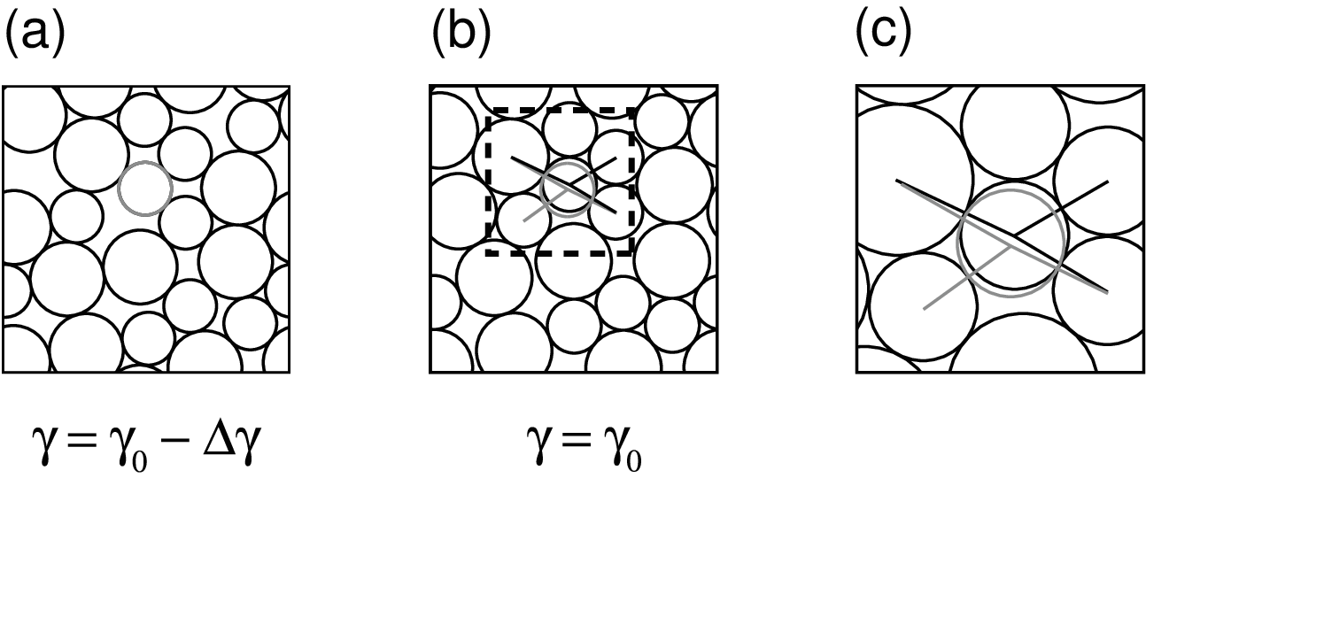
An example of a bifurcation in the energy landscape is shown in Fig. 20. This region of the landscape is extremely flat, and thus the state of the system will depend on the numerical precision and specific details of the energy minimization scheme. For example, if the energy minimization stops at point $a^{\prime}$ in Fig. 20, it will likely move toward MS packing $a$ during the packing-generation process, while if it stops at point $b^{\prime}$ , the system may proceed to MS packing $b$ .

The configurational view of the trajectory splitting mechanism in Fig. 19 is demonstrated in Fig. 21, where we show the configuration before and after the splitting event at $\gamma=\gamma_{0}$ . There are subtle differences in the position and interparticle contacts of a single particle in the central region of the cell at strains $\gamma_{0}-T$ (gray outline) and $\gamma_{0}$ (black outline). This small change in the contact network, which occurs in a flat region of the energy landscape, leads to large differences at subsequent values of shear strain. In this case, the cause of the flatness in the energy landscape stems from the fact that the directions ${\hat{r}}_{ij}$ for different contacting particles $j$ of a central particle $i$ are nearly collinear.

Similarly, if we add random displacements during quasistatic shear, we can create bifurcating trajectories $\phi_{J}(\gamma)$ . In Fig. 22, we show the evolution of $\phi_{J}(\gamma)$ for systems with and without added Gaussian random displacements with both systems initialized with the same MS packing at $\gamma=0$ . We find that the trajectory with noise deviates from the original trajectory at $\gamma\approx 0.2$ . Thus, noise is able to compete with the contracting mechanism to increase the fraction of dynamically sampled MS packings. In future studies, we will determine the fraction of MS packings visited as a function of the noise amplitude and system size.

Rattler particles can also lead to sensitivity to initial conditions. Small changes in the location of the rattler particle even in MS packings that otherwise have the same network of particle contacts can lead to large differences in subsequent contact networks if the rattler joins the connected network in different locations. This effect occurs because there is no energetic incentive for rattler particles to be located in any particular location within the confining void region as long as it does not overlap another particle. The influence of rattler particles on transition rates will also be assessed in future studies by varying the noise amplitude.

VIII Conclusions

In this work, we enumerated and classified the mechanically stable packings of bidisperse frictionless disks that occur as a function of the applied shear strain $\gamma$ . We showed that MS packings form continuous geometrical families defined by the network of particle contacts.

In addition, we studied the evolution of these systems during quasistatic shear strain at zero pressure to mimic the dynamics of slowly sheared granular media. For small systems $N<16$ , we found that the dynamics was deterministic and strongly contracting, i.e. if the system is initialized in an ensemble of MS packings, it will quickly contract to at most a few MS packing families. The strong contraction stems from an abundance of short families, a propensity for the system to undergo more jumps than kinks in $\phi_{J}(\gamma)$ , the fact that jumps only lead to increases in packing fraction, and the observation that families at higher packing fraction attract more jumps.

In our studies of system sizes $N>16$ , we began to see features of large systems, including a dramatic increase in the period of the periodic orbits and bifurcations that lead to the random splitting of trajectories ( $\phi_{J}$ vs. $\gamma$ ). We suggest that both the contraction and splitting mechanisms will persist in the large-system limit, and the fraction of MS-packing geometrical families that are visited in steady-state will depend on ratio of the splitting and contraction rates. In large systems, we suspect that the dynamics will focus the system onto sets of frequent MS-packing families with similar structural and mechanical properties, although much more work is required to quantify these claims.

Our long-term research objective is to develop a master-equation formalism to describe macroscopic slowly driven granular systems from the ‘bottom-up’ in terms of collections of small subsystems or microstates. In this manuscript, we took a significant step forward in this effort. We identified the types of microstates that can exist over the full range of shear strain and studied the probabilities with which they occur. This information can be used as input in the master-equation approach to calculate the contraction and splitting rates and ultimately the steady-state distributions of macroscale MS packings.

Acknowledgements.

Financial support from NSF grant nos. CBET-0348175 (GG, JB), DMR-0448838 (GG, CSO), and DMS-0835742 (CSO) is gratefully acknowledged. We also acknowledge generous amounts of CPU time from Yale’s Center for High Performance Computing. We thank S. Hilgenfeldt, G. Lois, M. Shattuck, and W. Zhang for insightful comments.

Appendix A Numerical details

In this appendix, we elaborate on technical details of the simulations not described in the main text. We include specific numerical parameters of the packing-generation protocol and the method to construct the complete geometrical family map.

Packing-generation protocol

In Sec. IV.1, we outlined our procedure to generate mechanically stable packings. Here, we provide some of the numerical parameters involved in the simulations. For the energy minimization, we employ the conjugate gradient technique [32], where the particles are treated as massless. The stopping criteria for the energy minimization ( $V_{t}-V_{t-1}<V_{\rm tol}=10^{-16}$ and $V_{t}<V_{\rm min}=10^{-16}$ , where $V_{t}$ is the potential energy per particle at iteration $t$ ) and the target potential energy per particle of a static granular packing ( $V_{\rm tol}<V<2V_{\rm tol}$ ) are the same as used in previous studies [17]. For the first compression or decompression step we use the packing-fraction increment $\Delta\phi=10^{-4}$ . Each time the procedure switches from expansion to contraction or vice versa, $\Delta\phi$ is reduced by a factor of $2$ . Using the packing generation procedure with these parameters, we are able to locate the jamming threshold in packing fraction $\phi_{J}$ to within $10^{-8}$ for each static packing over the full range of $\gamma$ . Since we implement an energy minimization technique with no inertia, we do not need to alter the stopping criteria to handle rattler particles, which possess fewer than three contacts and are not members of the force bearing network.

Geometrical Families

To construct the complete map of geometrical families, we divided the region $\gamma=[0,0.5]$ into small shear strain intervals $\gamma_{s+1}-\gamma_{s}\equiv\Delta\gamma=10^{-2}$ . For the range of system sizes $N=4$ to $20$ studied, this choice for $\Delta\gamma$ limited the number of rearrangement events to roughly one per shear strain interval. At each sampled shear strain $\gamma_{s}$ , we generated at least $N_{t}=10^{6}$ MS packings using random initial particle positions.

Two MS packings at different shear strains are considered to belong to the same geometrical family if they possess the same set of particle contacts. The particle contact networks of two MS packings can be distinguished by comparing the eigenvalues of their connectivity matrices $C_{ij}$ , where the $ij$ -th element of ${\bf C}$ is $1$ if particles $i$ and $j$ are in contact and $0$ otherwise. Two systems have the same contact network if all of the eigenvalues of their connectivity matrices are the same.

Appendix B Dynamical matrix

In this appendix, we calculate the elements of the dynamical matrix (9) for the repulsive linear spring potential (8). We employ slightly different notation for the dynamical matrix compared to (9) by separating the spatial $\alpha,\beta=x,y$ and particle $i,j=1,\cdots,N$ indexes. As given in Ref. [34], for pairwise, central potentials the dynamical matrix has the following form for the off-diagonal components $i\neq j$ :

M_{i\alpha,j\beta}=-\frac{t_{ij}}{r_{ij}}\left(\delta_{\alpha\beta}-{\hat{r}}_{ij\alpha}{\hat{r}}_{ij\beta}\right)-c_{ij}{\hat{r}}_{ij\alpha}{\hat{r}}_{ij\beta},

(11)

where $\hat{r}_{ij\alpha}$ is the $\alpha$ th component of ${\hat{r}}_{ij}$ ,

t_{ij}\equiv\frac{{\partial V(r_{ij})}}{{\partial r_{ij}}}=-\frac{\epsilon}{\sigma_{ij}}\left(1-\frac{{r_{ij}}}{{\sigma_{ij}}}\right)\Theta\left(\frac{{\sigma_{ij}}}{{r_{ij}}}-1\right),

(12)

and

c_{ij}\equiv\frac{{\partial^{2}V(r_{ij})}}{{\partial r_{ij}^{2}}}=\frac{\epsilon}{\sigma_{ij}^{2}}\Theta\left(\frac{{\sigma_{ij}}}{{r_{ij}}}-1\right).

(13)

In the calculation of $t_{ij}$ and $c_{ij}$ , we have ignored the $\delta$ -function contributions arising from cases when particles $i$ and $j$ are just touching with $r_{ij}=\sigma_{ij}$ . The diagonal components ( $i=j$ ) of the dynamical matrix are given by

M_{i\alpha,i\beta}=-\sum_{j=1,i\neq j}^{N}M_{i\alpha,j\beta}.

(14)

The shear-periodic boundary conditions only affect the definition of the separation $r_{ij}$ for particles near the edges of the simulation cell.

Appendix C Polarizations of MS packings

In this appendix, we provide details for generating different polarizations in simulations and determining which polarizations are distinct.

Table 5: The eight roto-inversion matrices

{\bf R}_{i}

in 2D that when applied to a given MS packing at integer values of shear strain generate the eight equivalent polarizations with identical eigenvalue lists of the dynamical matrix.

(1) $\left({\begin{array}[]{*{20}c}1&0\\ 0&1\\ \end{array}}\right)$	(2) $\left({\begin{array}[]{*{20}c}0&1\\ -1&0\\ \end{array}}\right)$	(3) $\left({\begin{array}[]{*{20}c}-1&0\\ 0&-1\\ \end{array}}\right)$	(4) $\left({\begin{array}[]{*{20}c}0&-1\\ 1&0\\ \end{array}}\right)$
(5) $\left({\begin{array}[]{*{20}c}0&1\\ 1&0\\ \end{array}}\right)$	(6) $\left({\begin{array}[]{*{20}c}-1&0\\ 0&1\\ \end{array}}\right)$	(7) $\left({\begin{array}[]{*{20}c}0&-1\\ -1&0\\ \end{array}}\right)$	(8) $\left({\begin{array}[]{*{20}c}1&0\\ 0&-1\\ \end{array}}\right)$

We will first describe the symmetries that MS packings possess under shear periodic boundary conditions in undeformed cells, since these symmetries affect the number and types of MS packings that can be obtained during shear. At integer shear strains, there are eight ‘polarizations’ all of which have the same list of eigenvalues of the dynamical matrix, but different eigenvectors. A given MS packing at integer shear strain (panel (1)) and its equivalent polarizations (panels (2)-(8)) are shown in Fig. 5. Each polarization with coordinates ${\vec{\xi}}_{i}$ in panel (i) in Fig. 5 can be obtained from the original MS packing ${\vec{\xi}}_{1}$ in panel (1) using

{\vec{\xi}}_{i}={\bf R}_{i}{\vec{\xi}}_{1},

(15)

where the eight roto-inversion matrices ${\bf R}_{i}$ with ${\rm det}{\bf R}_{i}=\pm 1$ in 2D are given in Table 5. In isotropically compressed systems these polarizations occur with equal probability. However, in systems subjected to shear strain, these polarizations will occur with different probabilities.

2D systems subjected to simple planar shear flow possess a discrete rotational symmetry; i.e. the system is unchanged when it is rotated by $\pi$ about an axis coming out of the page (i.e. apply ${\bf R}_{3}$ to a given MS packing) as shown in the bottom of Fig. 5. In panels (1)-(8) in Fig. 5, we see that polarizations $1$ and $5$ , $2$ and $6$ , $3$ and $7$ , and $4$ and $8$ are related by rotations by $\pi$ , and therefore will behave the same under simple planar shear. Thus, only four distinct polarizations at integer shear strains remain.

If the accumulated shear strain is half-integer, MS packings will have at most only two distinct polarizations. Only four roto-inversion transformations are consistent with shear-periodic boundary conditions, ${\bf R}_{3}$ , ${\bf R}_{6}$ , and ${\bf R}_{8}$ in Table 5. These transformations have been applied to the configuration (a) in Fig. 23 to generate the configurations (b)-(d). However, (a) and (b) and (c) and (d) are related by the shear symmetry operation (rotations by $\pi$ , ${\bf R}_{3}$ ), and thus only two distinct polarizations remain at half integer strains.

In general, there is only one polarization for all shear strains other than integer and half-integer. Moreover, the number of polarizations at integer (half-integer) strains can be smaller than four (two) if particular MS packings possess additional symmetries.

In simulations, we distinguish the polarizations of two MS packings by applying all possible roto-inversion transformations configurations consistent with the shear-periodic boundary conditions to a given MS packing. We then compare the eigenvector (corresponding to the smallest nonzero eigenvalue) of the second configuration to that for all of the roto-inverted configurations of the first and look for a match.

References

[1] M. Toiya, J. Stambaugh, and W. Losert, Phys. Rev. Lett. 93, 088001 (2004).
[2] O. Dauchot, G. Marty, and G. Biroli, Phys. Rev. Lett. 95, 265701 (2005).
[3] O. Pouliquen, M. Belzons, and M. Nicolas, Phys. Rev. Lett. 91, 014301 (2003).
[4] J. Zhang, T. S. Majmudar, A. Tordesillas, and R. P. Behringer, “Statistical properties of a 2D Granular Material Subjected to Cyclic Shear,” preprint (2009); xxx.lanl.gov/abs/0906.2416.
[5] M. Nicolas, P. Duru, and O. Pouliquen, Eur. Phys. J. E 3, 309 (2000).
[6] G. Marty and O. Dauchot, Phys. Rev. Lett. 94, 015701 (2005).
[7] G. H. Ristow, G. Strassburger, and I. Rehberg, Phys. Rev. Lett. 79, 833 (1997).
[8] E. R. Nowak, J. B. Knight, E. Ben-Naim, H. M. Jaeger, and S. R. Nagel, Phys. Rev. E 57, 1971 (1998).
[9] P. Philippe and D. Bideau, Europhys. Lett. 60, 677 (2002).
[10] J. Choi, A. Kudrolli, and M. Z. Bazant, J. Phys.: Condens. Matter 17, S2533 (2005).
[11] H. A. Makse and J. Kurchan, Nature 415, 614 (2002).
[12] I. K. Ono, C. S. O’Hern, D. J. Durian, S. A. Langer, A. J. Liu, and S. R. Nagel, Phys. Rev. Lett. 89, 095703 (2002).
[13] C. S. O’Hern, A. J. Liu, and S. R. Nagel, Phys. Rev. Lett. 93, 165702 (2004).
[14] C. Song, P. Wang, and H. A. Makse, Nature 453, 629 (2008).
[15] C. Song, P. Wang, and H. A. Makse, Proc. Nat. Acad. Sci. 102, 2299 (2005).
[16] S. Henkes and B. Chakraborty, Phys. Rev. E 79, 061301 (2009).
[17] G.-J. Gao, J. Blawzdziewicz, and C. S. O’Hern, Phys. Rev. E 74, 061304 (2006).
[18] N. Xu, J. Blawzdziewicz, and C. S. O’Hern, Phys. Rev. E 71 061306 (2005).
[19] G.-J. Gao, J. Blawzdziewicz, and C. S. O’Hern, Phil. Mag. B 87, 425 (2007).
[20] G.-J. Gao, J. Blawzdziewicz, C. S. O’Hern, and M. Shattuck, preprint (2009); xxx.lanl.gov/abs/0903.4941
[21] S. F. Edwards and R. B. S. Oakeshott, Physica A 157, 1080 (1989).
[22] M. Depken and R. Stinchcombe, Phys. Rev. E 71, 065102(R) (2005).
[23] G. Tarjus and P. Viot, Phys. Rev. E 69, 011307 (2004).
[24] A. Fierro, M. Nicodemi, and A. Coniglio, Phys. Rev. E 66, 061301 (2002).
[25] A. Barrat, V. Colizza, and V. Loreto, Phys. Rev. E 66, 011310 (2002).
[26] A. Barrat, J. Kurchan, V. Loreto, and M. Sellitto, Phys. Rev. Lett. 85, 5034 (2000).
[27] S. Henkes, C. S. O’Hern, and B. Chakraborty, Phys. Rev. Lett. 99, 038002 (2007).
[28] E. Bertin, K. Martens, O. Dauchot, and M. Droz, Phys. Rev. E 75, 031120 (2007).
[29] N. Xu and C. S. O’Hern, Phys. Rev. E 73, 061303 (2006).
[30] M. P. Allen and D. J. Tildesley, Computer Simulation of Liquids (Oxford University Press, New York, 1987).
[31] D. J. Evans and G. Morriss, Statistical mechanics of nonequilibrium liquids (Academic Press, London, 1990).
[32] W. H. Press, B. P. Flannery, S. A. Teukolsky, and W. T. Vetterling, Numerical Recipes in Fortran 77 (Cambridge University Press, New York, 1986).
[33] S. Torquato and F. H. Stillinger, J. Phys. Chem. B 105, 11849 (2001).
[34] A. Tanguy, J. P. Wittmer, F. Leonforte, and J.-L. Barrat, Phys. Rev. B 66, 174205 (2002).
[35] In our simulations we use the criterion $|m_{i}|>m_{\rm min}$ for nonzero eigenvalues, where $m_{\rm min}=10^{-6}$ is the noise threshold for our eigenvalue calculations. Also, eigenvalues are considered to be equal if they differ by less than the noise threshold $m_{\rm min}$ .
[36] B. A. Isner and D. J. Lacks, Phys. Rev. Lett. 96, 025506 (2006).
[37] D. J. Lacks and M. J. Osborne, Phys. Rev. Lett. 93, 255501 (2004).
[38] We estimate that only $\sim 60\%$ of the total number of distinct MS packings $N_{s}^{p}(\gamma)$ were found for $N=10$ .
[39] Short $\phi_{J}$ segments without parabolic-like vertexes also occur infrequently.
[40] We have also calculated the family length distribution using the eigenvalues of the connectivity matrix to determine the strains at which geometrical families begin and end, which is identical to the length distribution shown in Fig. 13 (a). (See Appendix A.)
[41] O. Reynolds, Phil. Mag. 20 469 (1885).
[42] A. Donev, R. Connelly, F. H. Stillinger and S. Torquato, Phys. Rev. E. 75, 051304, (2007).
[43] M. Mailman, C. F. Schreck, C. S. O’Hern, and B. Chakraborty, Phys. Rev. Lett. 102, 255501 (2009).
[44] Z. Zeravcic, N. Xu, A. J. Liu, S. R. Nagel, and W. van Saarloos, Europhys. Lett. 87, 26001 (2009).
[45] It is also possible that plotting $\phi_{J}$ does not adequately distinguish one MS packing from another; however, we have verified that the sequence of eigenvalue lists and polarizations at the beginning of the second cycle match those at the beginning of the first.