Derivation of the Langevin equation from the principle of detailed balance
Abstract
For a system at given temperature, with energy known as a function of a set of variables, we obtain the thermal fluctuation of the evolution of the variables by replacing the phase-space with a lattice and invoking the principle of detailed balance. Besides its simplicity, the asset of this method is that it enables us to obtain the Langevin equation when the phase-space is anisotropic and when the system is described by means of curvilinear coordinates. As an illustration, we apply our results to the Kramer–Watts-Tobin equation in superconductivity. The choice between the Itô and the Stratonovich procedures is discussed.
pacs
05.10.Gg, 05.40.-a, 74.40.+kI INTRODUCTION
In this article we deal with what we call “purely diffusive systems” in contact with a thermal bath. By this we mean systems with a state described by microscopic variables , with energy , which in the absence of thermal fluctuations are expected to follow an evolution equation
| (1) |
where is the time and the positive coefficients are determined by the dynamics of the system and its interaction with its environment. may be regarded as a driving force and as a compliance coefficient. The Langevin approach tells us that the influence of thermal fluctuations can be taken into account by adding a fluctuating quantity at the right hand side of the evolution equation; this fluctuating quantity is called the “Langevin term.”
The paradigm of a purely diffusive system is a particle that undergoes Brownian motion. In this case the variable is its momentum, is its kinetic energy and is the Stokes coefficient. Paul Langevin dealt with this problem[1] and determined the variance of the Langevin term by invoking the theorem of the equipartition of the kinetic energy among the various degrees of freedom of a system in thermal equilibrium. Gillespie[2] notes that it is not obvious that the influence of fluctuations can be separated as an additive term with zero average; regarding the velocity evolution as a Markovian process and assuming that the “stepping functions” (will be defined in the following section) are linear functions of velocity, it is shown that this separation indeed occurs. Katayama and Terauti[3] used the Langevin equation to study Brownian motion of a single particle under steady plane shear flow. Balescu[4] introduces a Langevin equation in a model for the description of a plasma. Bringuier[5] discusses the difficulties encountered when applying the Langevin approach to the Hall effect. The relation between the Langevin and the Klein–Kramers approaches is discussed in Ref. 6.
During the century that has elapsed since Langevin’s paper, his approach has been extended to wide classes of problems in Physics[7, 8, 9, 10] and the Langevin term is determined by means of the fluctuation-dissipation theorem.[11, 12, 13] In this paper we will evaluate the distribution of the Langevin term by means of the principle of detailed balance.[12]
The tools for handling the problems considered in this paper may be found in the literature on stochastic differential equations (e.g. Refs. 14, 15, 16) and many of the questions raised here may be avoided by switching to the Fokker-Planck equation; this article is addressed to those readers, pressumably physicists, who prefer a more intuitive approach.
II OUR METHOD
II.1 1D case
We consider a one-dimensional system with microscopic state determined by the variable . We discretize and assume that its possible values are , where is a “lattice constant.” We denote by the energy difference between consecutive lattice points. We assume now that for a short period of time the probability of passing from to is given by , where and are “stepping functions” that stand for the transition probability rates.
The principle of detailed balance asserts that in thermal equilibrium the probability for a transition from to equals that for a transition in the opposite direction, i.e., denoting by the equilibrium probability for the value , . Since , where is the Boltzmann constant and is the temperature,
| (2) |
It should be noted that not every system obeys detailed balance. Denoting by the probability for (not necessarily for equilibrium), stands for the probability current. Detailed balance requires that this current vanishes, whereas in order to mantain a stationary state it is sufficient that the divergence of the current vanishes. If probability currents are present in equilibrium, it follows that there are driving forces which cannot be expressed as the gradient of the energy as in Eq. (1) (such as the magnetic force on a charged particle). Therefore, systems that do not obey detailed balance are beyond the scope of this article.
In order to obtain more symmetric expressions, we write , and, taking sufficiently small so that quantities of order can be dropped, we write and , where and are at most of order . With this notation and approximation, Eq. (2) becomes
| (3) |
Similarly, requiring detailed balance between the sites and we obtain
| (4) |
where we have exchanged sides in the equation and neglected the difference . Multiplying the equations (3) and (4) and neglecting the term we obtain
| (5) |
hence is of order and will be dropped. can now be obtained from Eq. (3); keeping terms of order and making use of the definitions of and , it becomes
| (6) | |||||
where we have defined a smooth function such that .
Let us denote by the increment of the variable during the period of time . For sufficiently small we can neglect multiple transitions and the possible values of are 0 and . The average value of will be
| (7) |
where in the last step we have neglected higher orders of and have dropped the index . Similarly, the variance of will be
| (8) |
where besides dropping terms that are of higher order in we have used the fact that, for small , .
We now get rid of the unphysical lattice by defining . With this notation Eqs. (7) and (8) become
| (9) |
and
| (10) |
Finally, we consider a lapse of time which is very short compared with the relaxation time, but very long compared with . By the central limit theorem,[12, 17, 18] the increment of [which is the sum of many increments described by Eq. (9)] will be
| (11) |
where is a fluctuating term with average 0, variance and Gaussian distribution. is the Langevin distribution we were looking for. There is still a subtle question concerning the precise value of at which has to be evaluated; this issue is considered in Appendix A.
Let us now compare the nonfluctuating part of Eq. (11) with Eq. (1). If is independent of , Eq. (1) is recovered; otherwise, there is also a drift term that pushes towards values where is larger. The drift term can be absorbed into Eq. (1) if we replace the energy by . The term may be regarded as a sort of chemical potential, where plays the role of the activity.
II.2 Multivariable system
We consider now a system with variables . For each of the variables we can repeat the analysis of the previous section and Eq. (11) generalizes to
| (12) |
with and is a Langevin function with average 0, variance and Gaussian distribution.
We might also be interested in the evolution of other variables rather than those in the set . This problem is considered in Appendix B.
II.3 Curvilinear coordinates
Now the volume in phase space is proportional to the Jacobian of the coordinates; therefore, different lattice points in the discretized phase space may represent different volumes. As a consequence, has to be multiplied by this Jacobian and equations like Eq. (2) have to be modified accordingly. Before we deal with the general case, let us consider the case of polar coordinates.
II.3.1 Polar coordinates
Let the coordinates be , with volume element . For the variable the analysis remains unchanged, but for we have and equations like Eq. (2) have to be replaced with equations like
| (13) |
Following the steps of Sec. II.1, instead of Eq. (11) we now obtain
| (14) |
where has average 0, variance and Gaussian distribution. The replacement of the term with implies a drift towards larger values of .
It is tempting[19] to attribute the drift towards larger values of to the fluctuations of : if the system moves in phase space by the amount perpendicular to the radial direction, the new value of would be . After a lapse of time this effect would contribute an increment of by the amount . Comparison of this result with Eq. (14) indicates that this interpretation would be consistent with the principle of detailed balance only if .
II.3.2 General case
Let the coordinates be , with volume element . Then, when dealing with the transitions of the variable , Eq. (13) generalizes to
| (15) |
Following the steps of Sec. II.1, has an additional term and Eq. (14) generalizes to
| (16) |
where has average 0, variance and Gaussian distribution. An analogous result for macroscopic variables was obtained in Ref. 20.
A Mathematica-program that illustrates the use of this result is provided in Appendix C.
III Application—A model for superconductivity
One of the most useful models in the study of dynamic properties of superconductors is the time-dependent Ginzburg–Landau model.[21, 22] In this model the microstate of a superconductor is described by a complex field , such that is proportional to the density of superconducting electrons at position . Knowledge of the field enables us to evaluate several measurable quantities, such as the supercurrent density. Since in this model the variable of the problem is itself a field, it may provide an example in which the Langevin approach appears to be more practical than the Fokker-Planck equation, since the latter is a partial differential equation in a space with infinitely many dimensions.
In most cases, the time-dependent Ginzburg–Landau model is justified only for temperatures very close to the transition temperature. The model was generalized by Kramer and Watts-Tobin;[23] this generalized model is expected to be valid as long as there is local equilibrium. In order to focus on the aspects that we want to illustrate, we deal here with a simplified situation of the Kramer–Watts-Tobin model. We consider a uniform 1D superconductor with periodic boundary conditions and ignore the electromagnetic field. We discretize the system by dividing it into segments of equal length and denote by the value of at segment . With appropriate normalizations, the energy of the system is given by
| (17) |
where is a constant that depends on the material, the temperature, and the length of each segment. If fluctuations are ignored, the evolution of is given by[23]
| (18) |
where and are additional positive constants of the model.
Let us first consider the case , so that the left hand side in Eq. (18) can be approximated by . In this case it is convenient to express in Cartesian form, and the energy becomes . Performing the derivatives and separating real and imaginary parts, Eq. (18) takes the form
| (19) |
with , and an analogous equation is obtained for . Since is constant, we can apply the result (11) with no drift term and conclude that after time the fluctuating part of the increment of will have a variance .
Let us now consider the general situation. In this case it is convenient to express in polar form, , the energy becomes and the expression in brackets at the left hand side of Eq. (18) becomes . Multiplying Eq. (18) by and taking the real part we obtain the evolution of ,
| (20) |
taking the imaginary part gives the evolution of ,
| (21) |
These equations are in the form of Eq. (1), with and . In the extreme case , and . Since in this limiting situation does not depend on and does not depend on , the correction terms are not required and the formalism developed in Sec. II.3.1 can be applied with no drift terms. For general , thermal fluctuations add a drift to Eq. (20) and lead to
| (22) |
where is the usual Langevin term with variance .
It should be emphasized that Eq. (22) (including the drift) is an extension of Eq. (20) and not a modification of it. As an illustration of this statement, let us focus on the case already considered in Eq. (19). In this case the drift term becomes and becomes , i.e. . Moreover, let us for a moment leave the KWT model aside and consider the toy model , i.e., we just have instead of Eq. (18) and instead of Eq. (20). It follows that if the drift term were not present, the evolution equations for , and (including fluctuations) would all become identical and we would therefore have , whereas the true relationship is .
IV Conclusion
We have developed a simple method that enables us to derive the Langevin and drift terms for systems with random-walk type evolution. The cocepts of probability theory that we have invoked are intuitive, elementary and in the “language” used by undergraduate Physics textbooks. This method is particularly useful when the dynamics leads to an anisotropic phase space or when the evolution is naturally expessed in curvilinear coordinates.
Acknowledgements.
I have benefited from correspondence with Eric Bringuier, Moshe Gitterman, Peter Hänggi, Grzegorz Jung, Eduardo Mayer-Wolf, Zeev Schuss and Roman Vorobyov.Appendix A Itô or Stratonovich?
We first note that both terms in Eq. (11) are not of comparable sizes. The first is of order , whereas is . This does not mean that is more important, since it tends to cancel in the long run, whereas the first term persists.
The next question concerns the precise value of at which Eq. (11) should be evaluated. Should it be the initial value, , the final value , or some intermediate value? For the first term this question is irrelevant, since the change in the value of this term is and its contribution vanishes in the limit (even after noting that decreasing the time interval by some factor increases the number of intervals by the same factor). This is not the case for the choice of the -dependent variance of .
The Itô procedure evaluates the variance at . has a symmetric distribution and . The Stratonovich procedure evaluates the variance at the middle of the interval, . In order to distinguish between the two procedures, we denote the respective random terms by and . In order to fix ideas, let us explore the case that is an increasing function of . Since the variance is evaluated at , it means that if (respectively ), then (respectively ). Qualitatively, this means that the distribution of will have a longer tail than that of in the positive direction and a shorter tail in the negative direction.
In more quantitative terms, we can establish a one to one correspondence between the values of and those of , such that
| (23) |
where we have written as shorthand for and for at . The approximations in sequel (23) are , expansions to first order in , and . The important consequence is that for sufficiently small we have
| (24) |
This term is not negligible and does not cancel in the long run.
In a didactic article, van Kampen[24] explains how to translate between the Itô and the Stratonovich procedures. He advocates the use of a master equation rather than a Langevin approach, so that the Itô–Stratonovich dilemma never arises. Lançon et al. performed an experiment in which colloidal particles diffuse in a medium with position-dependend diffusion coefficient, so that . In their case they found that has to be evaluated at .
In order to judge what is the appropriate procedure for Eq. (11) in our case, we will evaluate . Since the difference between both procedures depends on and not on , we are free to take (we may imagine that is constant) and are left with a random walk problem in which each step is equally probable for both directions. Let the system be initially at ; by definition, the probability distribution for is the probability distribution for after time .
Let be the probability to find the system at at some moment. The change of probability after time will be . Or, defining ,
| (25) |
In order to use the central limit theorem, we require and we pass to a continuous model. Equation (25) becomes the diffusion equation
| (26) |
In order to pass from Eq. (25) to Eq. (26) we have expanded to order and used the definition of . Equation (26) may be regarded as our master equation.
Let us take the initial value . If in Eq. (26) were substituted by the constant , the solution of the diffusion equation would be
| (27) |
which is just the Itô distribution multiplied by . We now deal with Eq. (26) by means of the approximation
| (28) |
This nonhomogeneous equation is solved using the Green function of the diffusion equation.[26] We obtain that the deviation of the probability distribution from the Itô distribution is , where and the derivative is evaluated at . A plot of this deviation is shown in Fig. 1 [for any value of for which the approximations in Eq. (28) are justified].
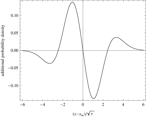
The deviation enhances the positive tail of the distribution of and hinders the negative tail, as in the case of . However, the key feature is that is not affected by ; therefore, has the appropriate distribution for our problem and the Itô procedure should be used. Also is not affected by . It is interesting to note that, no matter how small is, there are always values of where remains finite; however, the statistical weight of does become negligible in the limit of small .
Appendix B Linear transformation of variables
Let be the original set of variables for which the evolution of the system is known. Let us restrict ourselves to cases in which the coefficients are independent of the coordinates, so that . Let be a new set of variables, defined by means of a linear transformation
| (29) |
where are the elements of a constant orthogonal matrix ; the purpose of the factor is to compensate for the anisotropy of phase space.
Appendix C Numeric Test
In this Appendix we evaluate the statistical average of several quantities for a 2D system, using polar coordinates. In the following example we take an energy in which the Cartesian coordinates separate, namely, ; the statistical average of any function of will be and, similarly, and . The following is a Mathematica-program that evaluates several averages of this kind.
| theory, | 0.00 | 0.564 | 0.500 | 0.399 | 0.250 | 0.225 |
|---|---|---|---|---|---|---|
| numeric, | -0.01 | 0.561 | 0.493 | 0.402 | 0.253 | 0.227 |
| theory, | 0.00 | 0.798 | 1.000 | 0.564 | 0.500 | 0.450 |
| numeric, | -0.02 | 0.813 | 1.028 | 0.557 | 0.490 | 0.456 |
Clear[r, phi]; (* These are the polar coordinates *)
energy = r^2 (1 + Sin[phi]^2); (* This is the energy in polar coordinates *)
kT = 2; (* This is *)
Gammartau = 5.*^-4 r; Gammaphitau = 5.*^-5/r^2; (* These are and ; only the products of these quantities appear in each step; statistical averages should be independent of these dynamical functions, which have been chosen arbitrarily *)
stepr = Simplify[Gammartau D[kT Log[r Gammartau] - energy, r]]; (* This is as in Eq. (14) without *)
stepphi = Simplify[Gammaphitau D[kT Log[r Gammaphitau] - energy, phi]]; (* This is without *)
stdr = Simplify[Sqrt[2 kT Gammartau], Assumptions -> r > 0]; stdphi =
Simplify[Sqrt[2 kT Gammaphitau], Assumptions -> r > 0]; (* These are the standard deviations of and *)
r = 0.1; phi = 0.2; (* This is the initial microstate; the statistical averages should be independent of it *)
Nrelax = 5 10^6; (* Number of steps during which the system “forgets” the initial state and relaxes from it to a “typical” microstate *)
Do[r = r + stepr + RandomReal[NormalDistribution[0, stdr]]; (* evolves during a step, according to Eq. (14). stdr is evaluated at the beginning of the step, according to the Itô procedure *)
If[r < 0, r = -r; phi = phi - Pi]; (* If becomes negative, and are redefined *)
phi = phi + stepphi + RandomReal[NormalDistribution[0, stdphi]], (* evolves during a step, according to Sec. II.3.1. does not depend on , so that the stage at which stdphi is evaluated is not crucial *)
{i,Nrelax}]; (* Length of the loop *)
Naverage = 15 10^6; (* Number of steps during which averages will be evaluated *)
sx = 0; sxx = 0; sy = 0; syy = 0; sxy = 0; sabs = 0; (* Initialization of the variables that will be used for the evaluation of cumulative sums, from which the averages will be obtained; the following loop is identical to the one above, except that now we keep track of these sums *)
Do[r = r + stepr + RandomReal[NormalDistribution[0, stdr]];
If[r < 0, r = -r; phi = phi - Pi];
phi = phi + stepphi + RandomReal[NormalDistribution[0, stdphi]];
x = r Cos[phi]; y = r Sin[phi]; sxy = sxy + x y; x = Abs[x];
y = Abs[y]; sx = sx + x; sxx = sxx + x^2; sy = sy + y;
syy = syy + y^2; sabs = sabs + x y, {i, Naverage}];
Print["<xy>=", sxy/Naverage]; Print["<|x|>=",sx/Naverage];
Print["<x^2>=", sxx/Naverage]; Print["<|y|>=",sy/Naverage];
Print["<y^2>=", syy/Naverage]; Print["<|xy|>=",sabs/Naverage]; (* The averages that we decided to evaluate are printed *)
In Table 1 we compare the results obtained by this program with the expected statistical averages.
References
- [1] P. Langevin, “Sur la théorie du mouvement brownien,” C. R. Acad. Sci. (Paris) 146, 530–533 (1908). See also D. S. Lemons and A. Gythiel, “Paul Langevin’s 1908 paper On the Theory of Brownian Motion,” Am. J. Phys. 65, 1079–1081 (1997).
- [2] D. Gillespie, “Fluctuation and dissipation in Brownian motion,” Am. J. Phys. 61, 1077–1083 (1993).
- [3] Y. Katayama and R. Terauti, “Brownian motion of a single particle under shear flow,” Eur. J. Phys. 17, 136–140 (1996).
- [4] R. Balescu, “Stochastic transport in plasmas,” Eur. J. Phys. 21, 279–288 (2000).
- [5] E. Bringuier, “On the Langevin approach to particle transport,” Eur. J. Phys. 27, 373–382 (2006).
- [6] E. Bringuier, “From mechanical motion to Brownian motion, thermodynamics and particle transport theory,” Eur. J. Phys. 29, 1243–1262 (2008).
- [7] S. Chandrasekhar, “Stochastic problems in physics and astronomy,” Rev. Mod. Phys. 15, 1–89 (1943).
- [8] P. C. Hohenberg and B. I. Halperin, “Theory of dynamic critical phenomena,” Rev. Mod. Phys. 49, 435–479 (1977).
- [9] W.T. Coffey, Yu.P. Kalmykov and J.T. Waldron, The Langevin Equation: with Applications to Stochastic Problems in Physics, Chemistry, and Electrical Engineering 2nd ed. (World Scientific, Singapore, 2004).
- [10] J. Dunkel and P. Hänggi, “Relativistic Brownian motion,” Phys. Rep. 471, 1–73 (2009).
- [11] H. B. Callen and R. F. Greene, “On a theorem of irreversible thermodynamics,” Phys. Rev. 86, 702–710 (1952).
- [12] F. Reif, Fundamentals of Statistical and Thermal Physics (McGraw-Hill, Kogakusha, 1965).
- [13] R. Kubo, M. Toda, and N. Hashitsume, Statistical Physics II (Springer, Berlin, 1995).
- [14] R. L. Stratonovich, Conditional Markov Processes and Their Application to the Theory of Optimal Control (Elsevier, New York,1968).
- [15] Z. Schuss, Theory and Applications of Stochastic Differential Equations (Wiley, New York, 1980).
- [16] B. K. Øksendal, Stochastic Differential Equations 6th ed. (Springer, 2003).
- [17] A. I. Khinchin, Mathematical Foundations of Statistical Mechanics (Dover, New York, 1949) p. 166.
- [18] W. Feller, An Introduction to Probability Theory and its Applications, 2nd ed., Vol. II (Willey, New York, 1971).
- [19] M. Raible and A. Engel, “Langevin equation for the rotation of a magnetic particle,” Appl. Organometal. Chem. 18, 536–541(2004).
- [20] H. Grabert and S.M. Green, “Fluctuations and nonlinear irreversible processes,” Phys. Rev. A 19, 1747–1756 (1979), H. Grabert, R. Graham and S.M. Green, “Fluctuations and nonlinear irreversible processes II,” Phys. Rev. A 21, 2136–2146 (1980); for a readable summary see P. Hänggi, “Connection between deterministic and stochastic descriptions of nonlinear systems,” Helv. Phys. Acta 53, 491–496 (1980).
- [21] L. P. Gor’kov and G. M. Eliashberg, Zh. Eksp. Teor. Fiz. 54, 612–626 (1968) [“Generalization of the Ginzburg-Landau equations for non-stationary problems in the case of alloys with paramagnetic impurities,” Soviet Phys. JETP 27, 328–334 (1968)]; A. Schmid, “A time dependent Ginzburg–Landau equation and its application to the problem of resistivity in the mixed state,” Phys. Kondens. Mater. 5, 302–317 (1966).
- [22] M. Tinkham, Introduction to Superconductivity (Dover, 1996); N. B. Kopnin, Theory of Nonequilibrium Superconductivity (Oxford University, 2001).
- [23] L. Kramer and R. J. Watts-Tobin, “Theory of dissipative current-carrying states in superconducting filaments,” Phys. Rev. Lett. 40, 1041–1044 (1978); R. J. Watts-Tobin, Y. Krähenbühl, and L. Kramer, “Nonequilibrium theory of dirty, current-carrying superconductors: phase-slip oscillators in narrow filaments near ,” J. Low Temp. Phys. 42, 459–501 (1981).
- [24] N. G. van Kampen, “Itô versus Stratonovich,” J. Stat. Phys. 24, 175–187 (1981).
- [25] P. Lançon, G. Batrouni, L. Lobry, and N. Ostrowsky, “Brownian walker in a confined geometry leading to a space-dependent diffusion coefficient,” Physica A 304, 65–76 (2002).
- [26] A. D. Polyanin, Handbook of Linear Partial Differential Equations for Engineers and Scientists (Chapman & Hall/CRC, 2002).