Pokrovsky-Talapov Model at finite temperature: a renormalization-group analysis
Abstract
We calculate the finite-temperature shift of the critical wavevector of the Pokrovsky-Talapov model using a renormalization-group analysis. Separating the Hamiltonian into a part that is renormalized and one that is not, we obtain the flow equations for the stiffness and an arbitrary potential. We then specialize to the case of a cosine potential, and compare our results to well-known results for the sine-Gordon model, to which our model reduces in the limit of vanishing driving wavevector . Our results may be applied to describe the commensurate-incommensurate phase transition in several physical systems and allow for a more realistic comparison with experiments, which are always carried out at a finite temperature.
pacs
11.10.Gh, 11.10.Kk, 64.70.RhI Introduction
The Pokrovsky-Talapov[2, 1] (PT) model describes a large variety of systems displaying a commensurate/incommensurate (C/IC) transition, ranging from vortex depinning in type-II superconductors [3] to adsorbate layers on crystal surfaces [4] and quantum Hall bilayer systems under a tilted magnetic field. [5, 7, 6] This model is closely related to the sine-Gordon model,[8] with the extra feature of a characteristic driving wavevector imposed through the cosine term. In this work we present a functional renormalization group calculation of the finite-temperature corrections to the mean field results.
The Hamiltonian for the PT model is
| (1) |
where and . At mean-field level, one approximates the thermodynamic free energy by the Hamiltonian itself, evaluated at the field configuration that minimises the energy for given boundary conditions. This neglects the contributions of all fluctuations away from the minimum, therefore becoming less accurate as the temperature is raised and the entropic contribution of fluctuations increases. In this approximation, it is straightforward to compare the free energy of a configuration with the field following the driving wavevector (commensurate phase) to that of one in which the field no longer follows the imposed . As increases, the presence of the stiffness term, suppressing deviations of the field from uniformity, makes it more and more costly to remain in the commensurate phase, until a critical is reached at which the incommensurate phase becomes energetically favourable. The aim of this article is to investigate the effects of thermal fluctutations on this critical .
We shall use a functional renormalization group (RG) scheme to study the model at finite temperatures. Our approach is as follows: We perform a simple transformation which maps the PT model to a sine-Gordon model with additional terms depending only on the total topological “charge” of the system and on the driving wavevector . The RG transformation does not couple the sine-Gordon part to the -dependent part. Taking advantage of this, we renormalize the sine-Gordon part of the Hamiltonian and obtain a long-wavelength effective action, which we subsequently use to obtain the new value of the critical .
The main technical complication one faces in constructing a systematic renormalization group transformation for the sine-Gordon model is the inability to expand the cosine term in Eq. (1) in powers of the field and keep only a finite number of these. There are three main reasons for this complication: First, the periodicity of the cosine is crucial and is destroyed by any finite-order Taylor expansion. Second, we are interested in the two-dimensional case; as follows from simple power counting,[9, 8] polynomial interactions involving any power of the field are relevant in two dimensions. Finally, we are not interested in the fixed point of the RG transformation, but in the actual values of the various parameters after integrating out the degrees of freedom that we are not interested in.
Not expanding the cosine means that, in diagrammatic language, we ought to keep track of an infinite number of diagrams to one loop. This problem has already been solved for the case of the Wilsonian RG by F. Wegner and A. Houghton in Ref. 10, where these authors derive the eponymous exact renormalization group equation. This equation is also the limit of an approximate recursion relation first given by Wilson.[11] Wilson’s approximate recursion relation has been applied to the problem of critical wetting in Refs. [12, 13] because the effective field theories used in studying critical wetting share with our problem its dimensionality, preventing the use of the more usual perturbation methods. In general, functional renormalization group approaches are useful for cases where there is an effective potential with a nontrivial functional dependence on the field, such as the cosine term in Eq. (1).
The exact functional renormalization equation of Wegner and Houghton relies on a sharp, moving cutoff in momentum space. A sharp cutoff induces long-range interactions in real space and complicates the calculation of the flow of the stiffness in Eq. (1). This may be overcome by employing a smooth cutoff function;[14, 15] however, the resulting trajectories depend on the precise form of the cutoff. It has been shown[16] that the Wilsonian RG approach (of which the Polchinksi RG is an example) suffers from strong scheme dependence even in the asymptotic regime. Various alternative formulations of RG transformations exist that do not suffer from this problem; one that has recently been applied to the sine-Gordon model is the functional renormalization of the effective average action[17, 18] (EAARG) in which a transformation is obtained, not for the Hamiltonian itself, but for the generating function for the 1-particle irreducible Green’s functions. This is the RG scheme that we use in this article.
The outline of this paper is as follows: In Sec. II we describe the model and give a qualitative description of its behaviour. In Sec. III we explain the basic idea behind our approach before proceeding directly to the derivation (Sec. IV) and application to the PT model (Sec. V) of the appropriate RG flow equations. Finally, we give a brief discussion of our results in Sec. VI.
II The Model
To qualitatively understand the features exhibited by a system described by the PT Hamiltonian given in Eq. (1), consider first the case . It is then clear that, at mean field level, will simply remain at one of the minima of the potential at with
On the other hand, consider the quantity ; for low enough temperatures, it is given by the 1-loop result
| (2) |
in which , is a modified Bessel function and indicates a cumulant. Since if and , the right hand side of Eq. (2) diverges as , i. e., there is no long-range order in the system. This is merely an example of the Mermin-Wagner theorem.[8, 19] In addition, the system exhibits a Kosterlitz-Thouless type transition[19] on some line , which is again completely missed by a mean-field analysis.
This transition is analogous to the roughening transition in interface problems.[15, 20] In this analogy, the phase corresponds to the height of an interface above a reference level.11 1 That is, a noncompact variable; some complications from the compactness of are taken into account in Ref. [28]. The phase in which remains finite as is called the “smooth” phase, while the one in which diverges is called the “rough” phase. Given the value of at some arbitrary point which we take to be the origin, the value of at some other point arbitrarily far from it either remains within a finite distance from (smooth phase) or it does not but rather crosses over the maxima of . Clearly, the system with is in the rough phase;22 2 Note that the system also undergoes a KT transition between a phase with exponentially-decaying to one with algebraically-decaying correlations; this transition is different from the one we mention here and will not concern us in this work. the usual RG analysis of the sine-Gordon model, Eq. (1) with shows that, for given temperature and , there exists a below which the system is rough and above which it is smooth. For it is always smooth.
Consider now the case of finite . In the roughening picture, this corresponds to a potential that depends on the position ; as increases, the minima of the potential move to larger values of . In other words, the potential is effectively “tilted”. Thus, the potential part of the Hamiltonian tends to favour a that increases with position and follows the potential, (“commensurate phase”), while the gradient part favours a spatially constant (“incommensurate phase”). The competition between and leads to a transition between the two states as, for example, is varied.
Notice that there are two separate effects here: one is the roughening transition (belonging to the Kosterlitz-Thouless universality class), which is already present when and the other is the commensurate-incommensurate transition, which appears only for finite . These two effects may be conveniently separated out as described in the next section.
III Determination of at mean-field level
III.1 Separation of the Hamiltonian
We begin by shifting to the new variable , whereupon the Hamiltonian becomes
| (3a) | |||
| with | |||
| (3b) | |||
| (3c) | |||
| and | |||
| (3d) | |||
that is, the sum of the “charges” of all solitons present (per unit length); the integer simply indexes the soliton.
This form of the Hamiltonian is advantageous in that it consists of a sine-Gordon part, , which is independent of , plus the two terms in , which do depend on . This last term is the essential difference from a simple sine-Gordon model. As we shall see in Sec. IV, is unaffected by an RG transformation. This will form the basis of our treatment of finite temperature effects.
III.2 Determination of critical
We shall next compute the critical in the mean-field approximation; this will be straightforwardly extended to the renormalized case in Sec. V.
To obtain the critical , we notice that the transition from the commensurate to the incommensurate phase is signalled by the appearance of a finite soliton density with charge . We therefore calculate the excess energy per unit area of a configuration with a single soliton (with charge ) over that of one with no solitons, ; we denote this by . The part of the energy cost of a solitonic configuration due to is calculated in a standard way (sketched out in Appendix A) to be , hence . This quantity vanishes at the transition point, yielding a mean-field critical of [6]
| (4) |
Note that diverges as , implying that the system remains in the commensurate state for all momenta; this is in agreement with the discussion at the end of Sec. II, according to which the creation of solitons (hence the transition to the incommensurate state) is caused by the stiffness overcoming the tendency of the phase field to follow the minimum of the tilted potential.
IV Exact renormalization group equations
Various schemes have been developed to study renormalization group transformations of two dimensional field theories: In the theory of critical wetting, there have been several studies using this formulation of the RG, initially to first order in the potential [21] and then to all orders. [12] All these approaches have essentially used a local-potential approximation (LPA), in which the potential is allowed to change under coarse-graining, while the stiffness is not. The same method was later extended to a nonlocal model. [22] In the same context there has also been work in which the gradient term is renormalized in an approximate way. [13] The LPA is generally thought to be applicable to wetting problems because the anomalous dimension is expected to be zero.
In the present problem, on the other hand, it is clear that for vanishing one should obtain Kosterlitz-Thouless behaviour; furthermore, as discussed above, the quantity only couples to the number of solitons, which is conserved under the RG flow. Thus, the appropriate RG must capture the Kosterlitz-Thouless type of behaviour, which requires to flow under the transformation.
As mentioned above, we shall use the effective average functional RG scheme introduced by Wetterich[17] and applied recently to the sine-Gordon model.[18] For completeness, we outline the derivation of the exact flow equation for the effective action before applying it to the sine-Gordon model; for more details, see Refs. 17, 23, 18.
From this point onwards, we will subsume the temperature into the parameters and ; that is, we use units in which the temperature .
One begins by defining the bare action and adding to it a piece
where is called a regulator function (see below). One also adds a source term and writes . The quantity
is then the generator of connected correlation functions[9] for the action . Its Legendre transform is
where is the average of the field. We also define a new, related function
| (5) |
Using well-known[9] properties of and , and writing where is the initial value of the cutoff , one finds
| (6) |
with indicating the functional derivative of . This is an exact result.[17] It can be shown[17] that if as then : fluctuations about the mean-field solution are completely suppressed. Conversely, if as then , so that the full generator of 1 particle irreducible (1PI) vertices is obtained.
A full solution of Eq. (6) for would amount to computing all 1PI functions of the system at some length scale , including the full effects of fluctuations. This is not a simple problem, and one must resort to approximations. We will take the form of to be
A tedious but straightforward computation leads to[25, 24, 23]
| (7a) | ||||
| (7b) | ||||
where the operator projects the function to its right onto the field-independent functional subspace33 3 That is, . and . We take the cutoff function to be
| (8) |
The parameter controls the sharpness of the regulator function in both wavevector and real space: for large , is local in wavevector space and long-range in real space; for , it is instead smooth in momentum space but sharp in real space.
If is restricted to its leading Fourier component , the flow equations are, to leading-order and after rescaling,
with , reproducing the well-known leading-order flow equations for the sine-Gordon model.[27, 15, 26, 8]

Including higher-order terms on the right hand side of Eqs. (7a) and (7b) is, in principle, straightforward; for example, expanding in powers of and computing the integrals, one obtains
| (9) |
A similarly ungainly equation holds for . These expressions are greatly simplified if we make the choice in the regulator function Eq. (8). For the potential, the series on the right hand side of Eq. (9) may be summed (see Appendix B) to yield
Restricting the potential to the form we obtain the flow equation for [18]
| (10) |
(see Appendix B). In a similar way, and using the results of Appendix B to isolate the field-independent part, we obtain for the flow of
| (11) |
The flow diagram corresponding to Eqs. (10) and (11) is shown in Fig. (1).
We now turn to the application of the flow equations to the PT model.
V Application of RG to the PT model
V.1 Calculation of using the RG results
To determine the scale at which we may stop integrating the flow equations and use mean field theory, one may use the scale-dependent correlation length (see Eq. (2)) . Mean field theory applies if , while it is inapplicable otherwise. Thus, the appropriate at which integration may be stopped may be located by integrating up to the point at which is a minimum; the mean-field approach of Sec. III may then be used to determine . This is justified a posteriori if indeed . This condition is satisfied for all parameter values we have studied (see Fig. 2 for a representative example).

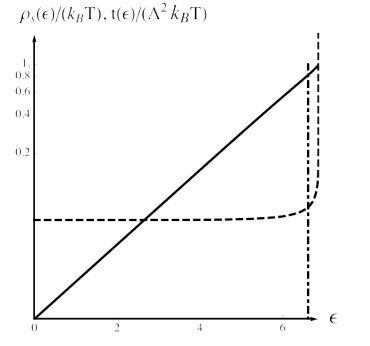
How would the calculation described in Sec. III be affected by the RG transformation? As we saw in Sec. IV, is invariant under the RG transformation, while is not, i. e., the parameters in will change to and , respectively. To obtain the critical , we notice that while is unaffected by the RG, the energy of a single soliton now depends on : we have . This results in an energy difference between the phase with no solitons and the phase with a single soliton given by . Setting this equal to zero and solving for , as in section III, yields
| (12) |
The factor ensures that we are using physical (as opposed to rescaled) units. Eq. (12) reduces to the correct mean-field expression, Eq. (4), for .
In Fig. 2 we show a representative plot of the evolution of with . Evidently, the minimum is well below so that mean field theory is applicable to the renormalized .
Let us now discuss the scheme-dependence of our calculation. In Ref. 16 it is shown that the trajectories resulting from the effective action functional RG scheme we use are scheme-independent, provided that the quantities and flow as powers of the parameter , i. e., with some (and similarly for ). They term the region in which this occurs the “freezing region”. Note that this scheme-independence does not hold in general for the case of Wilson-type renormalization.
Fig. 3 is a log plot of the evolution of and with . The full line is , the dashed line is and the dot-dashed line indicates the position of the minimum of (see also Fig. 2). Evidently, both and are in the freezing region at the values of that we are interested in. This happens for all initial values of and that we have checked.

V.2 Results and discussion
In Figs. 4 (a) and (b) we show the ratio determined by numerically integrating the flow equations and applying the method discussed above; this corresponds to the ratio . A darker colour indicates a larger decrease of the critical due to thermal effects (see the insets and notice the different scales). The plot in Fig. 4 (b) is a zoomed-in part of Fig. 4 (a) (notice the range of the axes and also the changed color coding).
For the purposes of this section, we will switch back to using natural units, by defining and , i. e., and are the parameters in physical units (while and are in units in which ).
First let us fix and and vary , i. e., fix and vary . For increasing (decreasing) , increases (decreases), vanishing as . This occurs because, as described in Sec. II, for vanishing there is no long-range order even in the absence of . This effect is not present at mean-field level, hence vanishes with decreasing .
Next, fix and and vary . From Fig. 4, increases (decreases) for decreasing (increasing) or .
Finally, consider fixing and and varying the temperature . This corresponds to fixed or, in terms of Fig. 4, to moving on rays emanating from the origin with gradient . Increasing (decreasing) the temperature corresponds to moving inwards (outwards) from the origin. As is increased, a will be reached at which the system will enter the rough phase at the extreme lower left corner of the diagram; thus, at high enough , vanishes for all and . Equivalently, this may be viewed as a proliferation of solitons because the RG flow there is such that monotonically as , so that we also have . This brings up the intriguing possibility of a purely temperature-driven commensurate-incommensurate transition in suitable systems. For low enough temperatures, as expected.
VI Conclusions
We have studied thermal effects on the commensurate-incommensurate transition point of the PT model using a renormalization-group approach. Our scheme relies on splitting the PT Hamiltonian into a sine-Gordon part, , and a part depending only on the number of solitons present, . We then derive a functional RG transformation which acts on the sine-Gordon part while leaving the soliton part invariant. We are thus able to determine the critical at which the incommensurate phase eventually becomes stable, taking into account thermal effects. We find a general lowering of compared to the mean-field result. Furthermore, there exists a regime in the - plane in which even for finite . This is due to the roughening transition, which is of Kosterlitz-Thouless type.
Since real experiments are performed at finite temperatures, the approach developed here may be applied to describe the C/IC transition in several physical systems. An application to the case of a Quantum Hall bilayer at total filling in the presence of a tilted magnetic field, motivated by recent experiments,[29] will be described in a forthcoming publication.[5]
Acknowledgements
We acknowledge financial support from the Netherlands Organization for Scientific Research (NWO) and thank L. K. Lim and N. Hasselmann for stimulating discussions. We also thank NORDITA for hospitality during the course of this work.
Appendix A Soliton energy
The excess energy of a single soliton may be calculated as follows: We have ; the solitonic profile satisfies the extremization condition . This condition gives an Euler-Lagrange equation, the first integral of which yields
| (13) |
Using this to eliminate the dependence of on the cosine term and changing the variable of integration we obtain
| (14) |
Finally, inserting Eq. (13) into Eq. (14) and integrating gives .
Appendix B Some trigonometric identities
It will be useful to know that
| (15) |
where the dots indicate higher-frequency Fourier components.
We begin by expanding the integrand of Eq. (7a) for ,
| (16) |
Finally, to restrict the flow of to the field-independent subspace, one needs the result
| (18) |
References
- [1] V. L. Pokrovsky and A. L. Talapov, Phys. Rev. Lett. 42, 65 (1979).
- [2] P. Bak, Rep. Prog. Phys. 45, 587 (1982).
- [3] T. Droese, R. Besseling, P. Kes and C. Morais-Smith, Phys. Rev. B 67, 064508 (2003).
- [4] R. Schuster, I. K. Robinson, K. Kuhnke, S. Ferrer, J. Alvarez and K. Kern, Phys. Rev. B 54, 17097 (1996).
- [5] O. Tieleman, A. Lazarides, D. Makogon and C. Morais Smith, in preparation.
- [6] C. B. Hanna, A. H. MacDonald and S. M. Girvin, Phys. Rev. B 63, 125305 (2001).
- [7] Kun Yang, K. Moon, L. Zheng, A. H. MacDonald, S. M. Girvin, D. Yoshioka and S.-C. Zhang, Phys. Rev. Lett. 72, 732 (1994); K. Moon, H. Mori, Kun Yang, S. M. Girvin and A. H. MacDonald, Phys. Rev. B 51 5138 (1995); Kun Yang, K. Moon, L. Belkhir, H. Mori, S. M. Girvin and A. H. MacDonald, Phys. Rev. B 54 11644 (1996).
- [8] C. Itzykson and J.-M. Druffe, Statistical Field Theory (Cambridge University Press).
- [9] D. J. Amit, Field Theory, the Renormalization Group and Critical Phenomena, Revised 2nd Edition (World Scientific).
- [10] F. Wegner and A. Houghton, Phys. Rev. A 8, 40 (1978).
- [11] K. G. Wilson and J. Kogut, Phys. Rep. 12, 75 (1974); K. G. Wilson, Phys. Rev. B 4, 3174 (1971); K. G. Wilson, Phys. Rev. B 4, 3184 (1971).
- [12] R. Lipowski and M. E. Fisher, Phys. Rev. B 36, 2126 (1987).
- [13] C. J. Boulter, Phys. Rev. E 57, 2062 (1998).
- [14] J. Polchinski, Nucl Phys. B231, 269 (1984).
- [15] D. A. Huse, Phys. Rev. B 30, 1371 (1984).
- [16] J.-I. Sumi, W. Souma, K.-I. Aoki, H, Terao and K. Morikawa, preprint hep-th/0002231.
- [17] C. Wetterich, Phys. Lett. B 301, 90 (1993); J. Berges, N. Tetradis and C. Wetterich, Phys. Rep. 363, 223 (2002).
- [18] S. Nagy, I. Nandori, J. Polonyi and K. Sailer, Phys. Rev. Lett. 102, 241603 (2009).
- [19] P. M. Chaikin and T. C. Lubensky, Principles of condensed matter physics (Cambridge University Press).
- [20] S. T. Chui and J. D. Weeks, Phys. Rev. B 14, 4978 (1976).
- [21] D. S. Fisher and D. A. Huse, Phys. Rev. B 32, 247 (1985).
- [22] A. O. Parry, J.-M. Romero-Enrique and A. Lazarides, Phys. Rev. Lett. 93, 086104 (2004).
- [23] J. Alexandre and J. Polonyi, Ann. Phys. (N. Y.) 288, 37 (2001).
- [24] V. Branchina, Phys. Rev. D 62 6330 (2000).
- [25] A. Bonanno, V. Branchina, H. Mohrbach and D. Zappala, Phys. Rev. D 60, 065009 (1999).
- [26] H. J. F. Knops and L. W. J. den Ouden, Physica 103A 597 (1980).
- [27] J. V. Jose, L. P. Kadanoff, S. Kirkpatrick and D. R. Nelson 16, 1217 (1977).
- [28] H. A. Fertig, Phys. Rev. Lett. 89, 035703 (2002); H. A. Fertig and K. Majumdar, Ann. Phys. 305, 190 (2003).
- [29] A. Fukuda, D. Terasawa, M. Morino, K. Iwata, S. Kozumi, N. Kumada, Y. Hirayama, Z. F. Ezawa and A. Sawada, Phys. Rev. Lett. 100, 016801 (2008)