Splitting of quantum information in traveling wave fields
using only linear optical elements

Entanglement is a commonplace of remarkable applications of Quantum Mechanics, such as quantum computation [2], superdense code [3], quantum teleportation [1], quantum communication via teleportation [4, 5], one-way quantum computation [6], quantum metrology [7] and so on. A state describing $N$ subsystems is entangled when it cannot be factorized into a product of $N$ states, each one concerning with a subsystem. In this respect, the $N$ subsystems are no longer independent, in spite of being spatially separated. As a consequence, a measurement upon one of them not only gives information about the other, but also provides possibilities of manipulating it [8].

There are various types of entangled states and classifying them is an arduous task, specially for multipartite systems [9]. However, Bennett et al. [10] shed light in this question through the use of the local operations and classical communication (LOCC) to define classes of equivalence in the set of entangled states, i.e, two entangled states belong to the same class of equivalence if one of them can be obtained from the other with certainty by means of LOCC. According to this criterion all bipartite pure-state entanglements are equivalent to that of the EPR type $(|00\rangle+|11\rangle)/\sqrt{2}$ [11]. Concerning with tripartite states, in Ref. [12] it was shown, via stochastic LOCC, that there are two genuine entanglement of tripartite systems: GHZ ($(|000\rangle\pm|111\rangle)/\sqrt{2}$) and W ($(|100\rangle+|010\rangle+|001\rangle)/\sqrt{3}$) states, i.e., W (GHZ) states cannot be converted into GHZ (W) states under stochastic LOCC. Although the canonical W states cannot be used for perfect teleportation and superdense coding, Ref. [13] introduced the following class of W states, suitable for these tasks,

	$\displaystyle|W_{\zeta}\rangle_{123}$	$\displaystyle=\frac{1}{\sqrt{2+2\zeta}}\left(|001\rangle_{123}+\sqrt{\zeta}e^{i\gamma}|010\rangle_{123}\right.$
		$\displaystyle+\left.\sqrt{\zeta+1}e^{i\delta}|100\rangle_{123}\right),$		(1)

where $\zeta$ is a real number and $\gamma$ and $\delta$ are phases. Latter on, in Ref. [14] the W states were generalized to multi-qubit and multi-particle systems with higher dimension. Recently, this class of W states has called attention of researchers, as exemplified in Ref. [15], in the context of QED-cavity. A procedure to split quantum information via W states was presented in Ref. [16]. This scheme relies on the following steps: i) the use of a three qubit W state previously prepared and shared by Alice, Bob, and Charlie; ii) a fourth qubit prepared in an unknown state (whose information we want to split) in Alice’s ownership; iii) a Bell-state measurement done by Alice and informing her result to Bob and Charlie; iv) the agreement between Bob and Charlie to send their particles, one to the other. After these steps, the splitting quantum state shared by Bob and Charlie can be reconstructed after an appropriate rotation.

In this brief report we show how to split a quantum state in the domain of running wave fields. Our scheme is experimentally feasible: it makes use of only linear optical elements, as beam splitters and phase shifters, plus photodetectors and one-photon sources. A very attractive scheme from the experimental point of view for generating the class of W states given by Eq.(1) is also presented. A W state of this class, required to split the quantum information, composes the nonlocal channel shared by Alice, Bob, and Charlie. Generation of W states in scenarios different from traveling waves has been proposed in Ref. [17]. The unknown quantum state used in our protocol to split the quantum information is

$$\left|\psi\right\rangle_{a}=C_{0}\left|0\right\rangle_{a}+C_{1}\left|1\right\rangle_{a}\text{ },$$

(2)

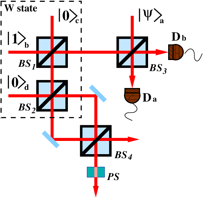
where $C_{0}$ and $C_{1}$ are coefficients that obey $\left|C_{0}\right|^{2}+\left|C_{1}\right|^{2}=1$. In Fig. 1 we show the experimental setup corresponding to our proposal.

W state generation - To engineer the desired W state we employ two $50/50$ beam splitters, as shown in the dashed region of Fig. 1. The initial state is given by $\left|\psi\right\rangle_{bcd}=\left|1\right\rangle_{b}\left|0\right\rangle_{c}\left|0\right\rangle_{d}$. After the interaction between modes $b-c$ in the $BS_{1}$ and modes $c-d$ in the $BS_{2}$, the state of the three qubits is

$$\left|\psi\prime\right\rangle_{bcd}=\frac{1}{\sqrt{2}}\left|1\right\rangle_{b}\left|0\right\rangle_{c}\left|0\right\rangle_{d}+\frac{i}{2}\left|0\right\rangle_{b}\left|1\right\rangle_{c}\left|0\right\rangle_{d}-\frac{1}{2}\left|0\right\rangle_{b}\left|0\right\rangle_{c}\left|1\right\rangle_{d}.$$

(3)

Note that the W state given by Eq.(3) is already of that class which leads to perfect teleportation and superdense coding with $\zeta=1$, $\gamma=3\pi/2$, and $\delta=\pi/2$ [13].

Quantum information splitting - To start our protocol for splitting the information, the state given by Eq.(2) is sent to Alice, who shares with Bob and Charlie an entangled state of the W type given by Eq.(3). The state of the whole system reads,

	$\displaystyle\left|\phi\right\rangle_{abcd}$	$\displaystyle=\frac{1}{2}\left(\sqrt{2}C_{0}\left|0,1,0,0\right\rangle_{abcd}+iC_{0}\left|0,0,1,0\right\rangle_{abcd}\right.$
		$\displaystyle-C_{0}\left|0,0,0,1\right\rangle_{abcd}+\sqrt{2}C_{1}\left|1,1,0,0\right\rangle_{abcd}$
		$\displaystyle+\left.iC_{1}\left|1,0,1,0\right\rangle_{abcd}-C_{1}\left|1,0,0,1\right\rangle_{abcd}\right).$		(4)

Alice now accomplishes a joint measurement on her qubits. The corresponding Bell-states are

	$\displaystyle|\Psi^{(\pm)}\rangle_{ab}$	$\displaystyle=$	$\displaystyle\frac{1}{\sqrt{2}}\left(\left|0,1\right\rangle_{ab}\pm i\left|1,0\right\rangle_{ab}\right),$		(5)
	$\displaystyle|\Phi^{(\pm)}\rangle_{ab}$	$\displaystyle=$	$\displaystyle\frac{1}{\sqrt{2}}\left(\left|1,1\right\rangle_{ab}\pm i\left|0,0\right\rangle_{ab}\right).$		(6)

After the Alice’s measurement, the state of the particles $c$ and $d$ on Charlie and Bob hands, respectively, collapses onto one of the entangled states appearing below (up to normalization)

			$\displaystyle\left.|\Psi^{\left(+\right)}\rangle_{ab}\left[\sqrt{2}C_{0}\left|0,0\right\rangle_{cd}+C_{1}\left(\left|1,0\right\rangle_{cd}+i\left|0,1\right\rangle_{cd}\right)\right]\right.$		(7)
		$\displaystyle+$	$\displaystyle|\Psi^{\left(-\right)}\rangle_{ab}\left[\sqrt{2}C_{0}\left|0,0\right\rangle_{cd}-C_{1}\left(\left|1,0\right\rangle_{cd}+i\left|0,1\right\rangle_{cd}\right)\right]$
		$\displaystyle+$	$\displaystyle|\Phi^{\left(+\right)}\rangle_{ab}\left[C_{0}\left(\left|1,0\right\rangle_{cd}+i\left|0,1\right\rangle_{cd}\right)+\sqrt{2}C_{1}\left|0,0\right\rangle_{cd}\right]$
		$\displaystyle+$	$\displaystyle\left.|\Phi^{\left(-\right)}\rangle_{ab}\left[C_{0}\left(\left|1,0\right\rangle_{cd}+i\left|0,1\right\rangle_{cd}\right)-\sqrt{2}C_{1}\left|0,0\right\rangle_{cd}\right]\right..$

Note that the two components are not symmetric: while one of them is a Bell state, the other one is a product state. The reconstruction of the state can be done provided that Bob and Charlie collaborate with each other. The $BS_{4}$, shown in Fig. 1, is used to decouple the states corresponding to modes $c-d$, as shown in the following. Fig. 2 shows the schematic circuit to generate the W state and to split quantum information.

Bell-state measurement - The Bell-state measurement carried out by Alice occurs in the $BS_{3}$ and in the photodetectors on modes $a$ and $b$. After this joint measurement the Bell-state evolves to

	$\displaystyle|\Psi^{(\pm)}\rangle_{a,b}$	$\displaystyle\rightarrow$	$\displaystyle\left\{\begin{array}[]{c}|1,0\rangle_{a,b}~~~~if~~~(+)\\ |0,1\rangle_{a,b}~~~~if~~~(-)\end{array}\right.,$
	$\displaystyle|\Phi^{(\pm)}\rangle_{a,b}$	$\displaystyle\rightarrow$	$\displaystyle\left\{|0,0\rangle_{a,b},~~|2,0\rangle_{a,b},~~or~~|0,2\rangle_{a,b}\right..$		(11)

Therefore, we can discern $|\Psi^{(+)}\rangle_{a,b}$ from $|\Psi^{(-)}\rangle_{a,b}$ by detecting either $|1,0\rangle_{a,b}$ or $|0,1\rangle_{a,b}$ on detectors $D_{a}$ and $D_{b}$, as shown in Fig. 1. Next, assuming for a moment that the detection corresponds to the states $|\Psi^{(\pm)}\rangle_{a,b}$, the state of the particles $c$ and $d$ can be written as

$$N(\sqrt{2}C_{0}\left|0,0\right\rangle_{cd}\pm C_{1}\left(\left|1,0\right\rangle_{cd}+i\left|0,1\right\rangle_{cd}\right)),$$

(12)

where $N$ stands for normalization. Now, after the interaction on $BS_{4}$ the states corresponding to modes $c$ and $d$ decouple in the form

$$|0\rangle_{c}(C_{0}\left|0\right\rangle_{d}\pm iC_{1}\left|1\right\rangle_{d}),$$

(13)

and a phase shift of $\pi/2$ ($3\pi/2$) cancels out the phase $i$ ($-i$), corresponding to the state $|\Psi^{(+)}\rangle_{a,b}$ ($|\Psi^{(-)}\rangle_{a,b}$). This step completes our protocol for splitting the quantum information via W states. Since we cannot distinguish between $|\Phi^{(+)}\rangle_{a,b}$ and $|\Phi^{(-)}\rangle_{a,b}$ the success probability for our protocol is $50\%$. In what follows we study how the fidelity of the process described by our protocol is influenced by nonidealities of beam splitters and photodetectors.

Losses in beam splitters and in photodetectors - For an ideal and symmetric beam splitter, the relationship between the input and the output operators can be written as

	$\displaystyle a_{in}^{{\dagger}}$	$\displaystyle\rightarrow$	$\displaystyle Ta_{out}^{{\dagger}}+iRb_{out}^{{\dagger}},$		(14)
	$\displaystyle b_{in}^{{\dagger}}$	$\displaystyle\rightarrow$	$\displaystyle Tb_{out}^{{\dagger}}+iRa_{out}^{{\dagger}},$		(15)

where $a^{{\dagger}}$ and $b^{{\dagger}}$ are the creation operators on modes $a$ and $b$, respectively, and the coefficients $T$ and $R$ satisfy the condition $T^{2}+R^{2}=1$. For the nonideal case, a phenomenological operator can be added in Eqs.(14 and 15) in a way that the relationship between the input and the output operators is given by [18]

	$\displaystyle a_{in}^{{\dagger}}$	$\displaystyle\rightarrow$	$\displaystyle ta_{out}^{{\dagger}}+irb_{out}^{{\dagger}}+\mathfrak{L}_{a}^{{\dagger}},$		(16)
	$\displaystyle b_{in}^{{\dagger}}$	$\displaystyle\rightarrow$	$\displaystyle tb_{out}^{{\dagger}}+ira_{out}^{{\dagger}}+\mathfrak{L}_{b}^{{\dagger}},$		(17)

where $t=\sqrt{\kappa}T$ and $r=\sqrt{\kappa}R$, with $t^{2}+r^{2}=\kappa$; $\mathfrak{L}_{i}$, $i=a,b$, are the Langevin operators accounting for the errors introduced by the fluctuating currents within the medium composing the $BS.$ The bosonic commutation relations for the output mode operators lead to the requirements for the Langevin operators: $[\mathfrak{L}_{a},\mathfrak{L}_{a}^{{\dagger}}]=[\mathfrak{L}_{b},\mathfrak{L}_{b}^{{\dagger}}]=\Gamma$ and $[\mathfrak{L}_{a},\mathfrak{L}_{b}^{{\dagger}}]=[\mathfrak{L}_{b},\mathfrak{L}_{a}^{{\dagger}}]=-\Delta$, where $\Gamma=1-\kappa$ is the damping constant and $\Delta=0$ for symmetric $BS$s. The ground-state expectation values for the products of pairs of Langevin operators are, for symmetric beam splitters, $\langle\mathfrak{L}_{a}\mathfrak{L}_{a}^{{\dagger}}\rangle=\langle\mathfrak{L}_{b}\mathfrak{L}_{b}^{{\dagger}}\rangle=\Gamma$, $\langle\mathfrak{L}_{a}\mathfrak{L}_{b}^{{\dagger}}\rangle=\langle\mathfrak{L}_{b}\mathfrak{L}_{a}^{{\dagger}}\rangle=0$, and $\langle\mathfrak{L}_{a}\rangle=\langle\mathfrak{L}_{a}^{{\dagger}}\rangle=\langle\mathfrak{L}_{b}\rangle=\langle\mathfrak{L}_{b}^{{\dagger}}\rangle=0$. The inefficiency of the photodetectors can be treated in a similar manner by relating the output operators to the input ones by [19]

$$a_{in}^{{\dagger}}\rightarrow\sqrt{\epsilon}a_{out}^{{\dagger}}+\mathrm{L}_{a}^{{\dagger}},$$

(18)

where $\epsilon$ stands for the detector efficiency. Note that, differently from the $BS$s, the detectors do not couple different modes [19]. Besides satisfying all properties introduced above, the Langevin operators $\mathrm{L}_{a}^{{\dagger}}$ also obey the commutation relations: $[\mathrm{L}_{a},\mathrm{L}_{a}^{{\dagger}}]=1-\epsilon$ and $[\mathrm{L}_{a},\mathrm{L}_{b}^{{\dagger}}]=0$; so the ground-state expectation values of their pair products are: $\langle\mathrm{L}_{a}\mathrm{L}_{a}^{{\dagger}}\rangle=1-\epsilon$ and $\langle\mathrm{L}_{a}\mathrm{L}_{b}^{{\dagger}}\rangle=0$.

Next, we turn to the procedure for splitting the quantum information, now including the loss effects. Let us begin by considering the input state

$$|\psi_{1}\rangle=(C_{0}\left|0\right\rangle_{a}+C_{1}\left|1\right\rangle_{a})\left|1,0,0\right\rangle_{bcd}\left|\mathbf{0}\right\rangle_{R},$$

(19)

as shown in Fig. 1. Here $\left|\mathbf{0}\right\rangle_{R}\equiv\prod\limits_{k}\left|0\right\rangle_{k}$ stands for the state of the environment composed of a huge number of vacuum-field states $\left|0\right\rangle_{k}$. In the following, this state impinges on the four beam splitters of the apparatus. In the first beam splitter ($BS_{1}$) the modes $a$ and $b$ become entangled, the whole system being described by

	$\displaystyle|\psi_{2}\rangle$	$\displaystyle=(C_{0}\left|0\right\rangle_{a}+C_{1}\left|1\right\rangle_{a})\left(t\left|1,0,0\right\rangle_{bcd}\right.$
		$\displaystyle+\left.ir\left|0,1,0\right\rangle_{bcd}+\mathfrak{L}_{1}^{{\dagger}}\left|0,0,0\right\rangle_{bcd}\right)\left|\mathbf{0}\right\rangle_{R}.$		(20)

After $BS_{2}$, the state $|\psi_{2}\rangle$ evolves to

	$\displaystyle|\psi_{3}\rangle$	$\displaystyle=(C_{0}\left|0\right\rangle_{a}+C_{1}\left|1\right\rangle_{a})\left(t\left|1,0,0\right\rangle_{bcd}\right.$
		$\displaystyle+\left.irt\left|0,1,0\right\rangle_{bcd}-r^{2}\left|0,0,1\right\rangle_{bcd}\right.$
		$\displaystyle+\left.ir\mathfrak{L}_{2}^{{\dagger}}\left|0,0,0\right\rangle_{bcd}+\mathfrak{L}_{1}^{{\dagger}}\left|0,0,0\right\rangle_{bcd}\right)\left|\mathbf{0}\right\rangle_{R}.$		(21)

After the $BS_{3}$, and including the effects of losses in the photodetectors via Eq.(18), we obtain the density operator for the whole system in the form

	$\displaystyle\rho$	$\displaystyle=$	$\displaystyle\left|0,1\right\rangle_{ab}\left\langle 0,1\right||\chi^{(01)}\rangle_{cdR}\langle\chi^{(01)}|$		(22)
			$\displaystyle+\left|1,0\right\rangle_{ab}\left\langle 1,0\right||\chi^{(10)}\rangle_{cdR}\langle\chi^{(10)}|+\rho_{res},$

where $|\chi^{(01)}\rangle_{cdR}$ and $|\chi^{(10)}\rangle_{cdR}$ are the states corresponding to modes $c$, $d$, and reservoirs when the modes $a$ and $b$ are described by $\left|0,1\right\rangle_{ab}$ and $\left|1,0\right\rangle_{ab}$, respectively; $\rho_{res}$ is the residual density operator, corresponding to the rejected terms in the detection by $D_{a}$ and $D_{b}$, i.e.,

$${}_{ab}\left\langle 0,1\right|\rho_{res}\left|0,1\right\rangle_{ab}=_{ab}\left\langle 1,0\right|\rho_{res}\left|1,0\right\rangle_{ab}=0,$$

(23)

since the detection of $\left|0,1\right\rangle_{ab}$ or $\left|1,0\right\rangle_{ab}$ are the sole possibilities that allow us to continue with the protocol, according to Eqs.(Splitting of quantum information in traveling wave fields
using only linear optical elements,11).

Following the ideal protocol explained above, we assume that Charlie and Bob agree in collaborating for the reconstruction of the state. After they send their particles to interact through the $BS_{4}$ we have the following evolutions $\left|\chi^{\left(01\right)}\right\rangle_{cdR}\rightarrow\left|\eta^{\left(01\right)}\right\rangle_{cdR}$ and $\left|\chi^{\left(10\right)}\right\rangle_{cdR}\rightarrow\left|\eta^{\left(01\right)}\right\rangle_{cdR}$, where

	$\displaystyle|\eta^{(01)}\rangle_{cdR}$	$\displaystyle=$	$\displaystyle\mathcal{N}_{01}\left\{\left[C_{0}\sqrt{\epsilon}t^{2}+2iC_{1}rt^{3}\sqrt{\epsilon}\mathrm{L}_{2}^{{\dagger}}\right.\right.$		(24)
			$\displaystyle+iC_{1}rt^{2}\sqrt{\epsilon}\mathfrak{L}_{3}^{{\dagger}}+C_{1}t^{3}\sqrt{\epsilon}\mathfrak{L}_{3}^{{\dagger}}$
			$\displaystyle-C_{1}r^{2}t\sqrt{\epsilon}\mathfrak{L}_{4}^{{\dagger}}-iC_{1}r^{3}\sqrt{\epsilon}\mathfrak{L}_{4}^{{\dagger}}$
			$\displaystyle\left.-C_{1}r^{2}\sqrt{\epsilon}\mathfrak{L}_{2}^{{\dagger}}+iC_{1}r\sqrt{\epsilon}\mathfrak{L}_{1}^{{\dagger}}\right]\left|0,0\right\rangle_{cd}\left|\mathbf{0}\right\rangle_{R}$
			$\displaystyle+\left[C_{1}r^{4}\sqrt{\epsilon}-C_{1}r^{2}t^{2}\sqrt{\epsilon}\right]\left|1,0\right\rangle_{cd}\left|\mathbf{0}\right\rangle_{R}$
			$\displaystyle-\left.2iC_{1}r^{3}t\sqrt{\epsilon}\left|0,1\right\rangle_{cd}\left|\mathbf{0}\right\rangle_{R}\right\},$

and

	$\displaystyle|\eta^{(10)}\rangle_{cdR}$	$\displaystyle=$	$\displaystyle\mathcal{N}_{10}\left\{\left[iC_{0}rt\sqrt{\epsilon}+2iC_{1}rt^{3}\sqrt{\epsilon}\mathrm{L}_{1}^{{\dagger}}\right.\right.$		(25)
			$\displaystyle+C_{1}t^{3}\sqrt{\epsilon}\mathfrak{L}_{3}^{{\dagger}}+iC_{1}rt^{2}\sqrt{\epsilon}\mathfrak{L}_{3}^{{\dagger}}$
			$\displaystyle+iC_{1}rt^{2}\sqrt{\epsilon}\mathfrak{L}_{4}^{{\dagger}}-C_{1}r^{2}t\sqrt{\epsilon}\mathfrak{L}_{4}^{{\dagger}}$
			$\displaystyle+\left.iC_{1}rt\sqrt{\epsilon}\mathfrak{L}_{2}^{{\dagger}}+C_{1}t\sqrt{\epsilon}\mathfrak{L}_{1}^{{\dagger}}\right]\left|0,0\right\rangle_{cd}\left|\mathbf{0}\right\rangle_{R}$
			$\displaystyle+\left[iC_{1}rt^{3}\sqrt{\epsilon}-iC_{1}r^{3}t\sqrt{\epsilon}\right]\left|1,0\right\rangle_{cd}\left|\mathbf{0}\right\rangle_{R}$
			$\displaystyle-\left.2C_{1}r^{2}t^{2}\sqrt{\epsilon}\left|0,1\right\rangle_{cd}\left|\mathbf{0}\right\rangle_{R}\right\},$

$\mathcal{N}_{01}$ and $\mathcal{N}_{10}$ standing for normalization. Then, as done in the ideal protocol, a phase shift is applied on mode $d$ to change the phase according to the detected state, in a way that $\left|0,1\right\rangle_{ab}$ ($\left|1,0\right\rangle_{ab}$) needs a phase shift of $3\pi/2$ ($\pi/2$).

Let us consider the case when Alice detects the state $\left|0,1\right\rangle_{ab}$. Then the density operator is reduced to the subsystems $c-d-R$ in the form

$$\rho_{cdR}^{(01)}=|\eta^{(01)}\rangle_{cdR}\langle\eta^{(01)}|.$$

(26)

Next, we trace out the reservoir in the operator above to get the fidelity $F_{01}=_{cd}\left\langle\Phi\right|\rho_{cd}^{(01)}\left|\Phi\right\rangle_{cd}$, with $\rho_{cd}^{(01)}=Tr_{R}(\rho_{cdR}^{(01)})$ and $\left|\Phi\right\rangle_{cd}=\left|0\right\rangle_{c}(C_{0}\left|0\right\rangle_{d}+C_{1}\left|1\right\rangle_{d})$:

	$\displaystyle F_{01}$	$\displaystyle=$	$\displaystyle\mathcal{N}_{01}^{2}\left[C_{0}^{4}\epsilon t^{4}+2C_{0}^{2}C_{1}^{2}\epsilon r^{3}t^{3}+4C_{0}^{2}C_{1}^{2}r^{2}t^{6}\epsilon(1-\epsilon)\right.$		(27)
			$\displaystyle+C_{0}^{2}C_{1}^{2}r^{2}t^{4}\epsilon(1-\kappa)+C_{0}^{2}C_{1}^{2}t^{6}\epsilon(1-\kappa)$
			$\displaystyle+2C_{0}^{2}C_{1}^{2}r^{3}t^{3}\epsilon+4C_{1}^{4}r^{6}t^{2}\epsilon+C_{0}^{2}C_{1}^{2}r^{4}t^{2}\epsilon(1-\kappa)$
			$\displaystyle+C_{0}^{2}C_{1}^{2}r^{6}\epsilon(1-\kappa)+C_{0}^{2}C_{1}^{2}r^{4}\epsilon(1-\kappa)$
			$\displaystyle+\left.C_{0}^{2}C_{1}^{2}r^{2}\epsilon(1-\kappa)\right]\text{,}$

where the normalization factor is

	$\displaystyle\mathcal{N}_{01}$	$\displaystyle=$	$\displaystyle\left[C_{0}^{2}t^{4}\epsilon+4C_{1}^{2}r^{2}t^{6}\epsilon(1-\epsilon)+C_{1}^{2}r^{2}t^{4}\epsilon(1-\kappa)\right.$		(28)
			$\displaystyle+C_{1}^{2}t^{6}\epsilon(1-\kappa)+4C_{1}^{2}r^{6}t^{2}\epsilon+C_{1}^{2}r^{4}t^{2}\epsilon(1-\kappa)$
			$\displaystyle+C_{1}^{2}r^{6}\epsilon(1-\kappa)+C_{1}^{2}r^{4}\epsilon(1-\kappa)$
			$\displaystyle+\left.C_{1}^{2}r^{2}\epsilon(1-\kappa)\right]^{-1/2}\text{.}$

Considering symmetric $BSs$ ($50/50$), where $t_{i}=r_{i}=\sqrt{\kappa/2}$, and current experimental parameters [19], e.g., $0.98\leq\kappa\leq 1$ and $0.7\leq\epsilon\leq 1$, we find $0.72\leq F_{01}\leq 1$. Fig. 2a shows the fidelity $F_{01}$ for a fixed $\kappa=0.98$ and varying $\epsilon$ and $C_{0}$. Fig. 2b shows the same for a fixed $\epsilon=0.7$ and varying $\kappa$ and $C_{0}$ whereas Fig. 3a corresponds to the worst case, for $\kappa=0.98$ and $\epsilon=0.7$, and varying $C_{0}$. To clarify the relevance of the photodetectors efficiency, Fig. 3b shows the fidelity for $\kappa=0.98$ and $\epsilon=1$ (ideal detectors).

In conclusion, we have proposed a simple and feasible scheme to split the quantum information encoded in a Fock state superposition in traveling waves. In addition, we show how to engineer a class of W states suitable for perfect quantum teleportation and superdense coding, with $100\%$ success probability, making use of an oversimplified scheme. Our whole scheme to split quantum information makes use of only linear optical elements and can be accomplished through a couple of detectors, four beam splitters, one phase shifter, and two single-photon sources. The errors introduced by nonidealities of the beam splitters and detectors were studied; in this case the fidelity of the state results better than that in the classical limit, even for the worst choice of experimental parameters concerned with the efficiency of detectors and losses in the beam splitters.

We thank the CAPES, CNPq, and FUNAPE/GO, Brazilian agencies, for the partial supports.

References

[1] C. H. Bennett, G. Brassard, C. Crépeau, R. Jozsa, A.
Peres, and W. K. Wootters, Phys. Rev. Lett. 70, 1895 (1993).
[2] M. A. Nielsen and I. L. Chaung, Quantum Computation
and Quantum Information (Cambridge University Press, Cambridge, 2000); D.
Gottesman and I. L. Chuang, Nature (London) 402, 390 (1999); E.
Knill, R. Laamme, and G. J. Milburn, Nature 409, 46 (2001).
[3] C. H. Bennett and S. J. Wiesner, Phys. Rev. Lett.
69, 2881 (1992).
[4] J. I. Cirac, P. Zoller, H. J. Kimble, and H. Mabuchi,
Phys. Rev. Lett. 78, 3221 (1997), and refs. therein.
[5] G. Brassard, S. L. Braunstein, and R. Cleve, Physica D
120, 43 (1998).
[6] R. Raussendorf and H. J. Briegel, Phys. Rev. Lett.
86, 5188 (2001).
[7] A. Gilchrist, K. Nemoto, W. J. Munro, T. C. Ralph, S.
Glancy, S. L. Braunstein, and G. J. Milburn, J. Opt. B: Quantum Semiclass.
Opt. 6, S828 (2004).
[8] R. Horodecki, P. Horodecki, M. Horodecki, and K.
Horodecki, Rev. Mod. Phys. 81, 865 (2009).
[9] Dagmar Bru and Gerd Leuchs, Lectures on
Quantum Information.
[10] C. H. Bennett et al., Phys. Rev. A 63,
012307 (2000).
[11] A. Einstein, B. Podolsky, and N. Rosen, Phys. Rev. A
47, 777 (1935).
[12] W. Dür, G. Vidal, and J. I. Cirac, Phys. Rev. A
62, 062314 (2000).
[13] P. Agrawal and A. Pati, Phys. Rev. A 74,
062320 (2006).
[14] L. Li and D. Qiu, J. of Phys. A: Math. Theor. 40, 10871 (2007).
[15] E. M. Becerra-Castro, W. B. Cardoso, A. T.
Avelar, and B. Baseia, J. Phys. B: At. Mol. Opt. Phys. 41, 215505
(2008).
[16] Shi-Biao Zheng, Phys. Rev. A 74, 054303 (2006).
[17] X. B. Zou, K. Pahlke, and W. Mathis, Phys. Rev. A
66, 044302 (2002); H. Mikami, Y. Li, and T. Kobayashi, Phys. Rev. A
70, 052308 (2004); H. Mikami, Y. Li, K. Fukuoka, and T. Kobayashi,
Phys. Rev. Lett. 95, 150404 (2005).
[18] S. Barnett, J. Jeffers, and A. Gatti, Phys. Rev. A
57, 2134 (1998).
[19] R. M. Serra, C. J. Villas-Bôas, N. G. de Almeida,
and M. H. Y. Moussa, J. Opt. B: Quantum Semiclass Opt. 4, 316