跳到论文正文
W Papers独立论文阅读器 arXiv:0909.0407 论文正文 计算阅读时间 · 0%
引用这篇论文根据当前论文元数据生成,正式投稿前建议核对。


License: arXiv.org perpetual non-exclusive license
arXiv:0909.0407v1 [hep-th] 02 Sep 2009

WIS/11/09-AUG-DPP

The 2-loop partition function of large NN gauge theories with adjoint matter on S3S^{3}

Matan Mussel, Ran Yacoby11 1 Emails: matan.mussel@weizmann.ac.il, ran.yacoby@weizmann.ac.il

Department of Particle Physics,
Weizmann Institute of Science,
Rehovot 76100, Israel

ABSTRACT

We compute the 2-loop thermal partition function of Yang-Mills theory on a small 3-sphere, in the large NN limit with weak ’t Hooft coupling λ=gY​M2​N\lambda=g_{YM}^{2}N. We include NsN_{s} scalars and NfN_{f} chiral fermions in the adjoint representation of the gauge group (S)​U​(N)(S)U(N), with arbitrary Yukawa and quartic scalar couplings, assuming only commutator interactions. From this computation one can extract information on the perturbative corrections to the spectrum of the theory, and the correction to its Hagedorn temperature. Furthermore, the computation of the 2-loop partition function is a necessary step towards determining the order of the deconfinement phase transition at weak coupling, for which a 3-loop computation is needed.

1 Introduction

1.1 Overview and outline

The interest in the thermodynamics of large NN Yang-Mills (YM) theories on a small 3-sphere S3S^{3}, originates in [1]. In that paper, the AdS/CFT correspondence [2, 3, 4] was used to study the thermal behavior of 𝒩=4\mathcal{N}=4 supersymmetric Yang-Mills theory (SYM) on S3S^{3}, with gauge group (S)​U​(N)(S)U(N). As the correspondence dictates, in the large NN limit with strong ’t Hooft coupling λ=gY​M2​N\lambda=g_{YM}^{2}N, this behavior can be found by studying classical type IIB supergravity. This study showed that the theory has a low temperature confining phase, in which the free energy scales as N0N^{0}, and a high temperature deconfining phase, in which the free energy scales as N2N^{2}. The two phases were found to be separated by a first order phase transition.

It is then interesting to ask whether this behavior persists even at small ’t Hooft coupling. In that limit the conformal 𝒩=4\mathcal{N}=4 theory can be studied by using perturbation theory. However the study needs not be restricted to weakly coupled conformal theories, and can be extended to asymptotically free YM theories. As opposed to conformal field theories, asymptotically free gauge theories generate an infrared scale ΛY​M\Lambda_{YM} which leads to the breakdown of perturbation theory in flat space at low temperatures/energy scales. But on S3S^{3} with radius RS3R_{S^{3}} that bad infrared behavior is cut off by the finite size of space, i.e. if RS3​ΛY​M≪1R_{S^{3}}\Lambda_{YM}\ll 1 one can use perturbation theory to compute the partition function at all temperatures.

This has been done in [5],[6], where it was shown that for a wide class of models the first order deconfinement transition persists even in the limit of zero ’t Hooft coupling. The phase transition is signaled by a Hagedorn behavior [7] near the critical temperature, where the density of states grows exponentially with energy. This remarkable behavior can be ascribed to a zero mode of the gauge field (i.e. a mode with vanishing quadratic action) which cannot be integrated out in perturbation theory. Gauge invariance highly constrains the low energy effective action of this mode, resulting in non-trivial self interactions for it even at zero coupling.

To order λ\lambda the phase transition is of first order and the critical temperature is identical with the Hagedorn temperature. However, in the next order in perturbation theory [6], the transition might be of first order and slightly below the Hagedorn temperature, or second order and at the Hagedorn temperature. In order to determine the order of the phase transition one needs to perform a 3-loop computation in perturbation theory. For pure YM this has been done in [8], where it was found that the transition is of first order. For YM theories with adjoint matter fields (including 𝒩=4\mathcal{N}=4 SYM) the order of the phase transition at weak coupling is still an open question and examples which exhibit either behavior can be easily constructed.

In this work we take a step further towards answering this question, by computing in perturbation theory the 2-loop partition function of (S)​U​(N)(S)U(N) YM theory in the large NN limit with fixed, small ’t Hooft coupling on S3S^{3}. We include scalars and chiral fermions in the adjoint representation of the gauge group with arbitrary Yukawa and quartic scalar couplings, only assuming commutator interactions (though our computation can be easily generalized to include non-commutator interactions as well). Our computation follows closely the one of [9] where the same computation was done for pure YM.

As an immediate application we can compute the order λ\lambda corrections to the Hagedorn temperature and to the spectrum of the theory. We check our computation by comparing to the known results for 𝒩=4\mathcal{N}=4 SYM, which were computed by spin-chain methods in [10].

The structure of this paper is as follows. In the next subsection we review some of the theoretical background necessary for this work. Section 2 reviews our conventions for the action, and various mode expansions on S3S^{3}. In section 3 we discuss our renormalization scheme, and present the computation of the various counterterms. In section 4 we present the computation of the 2-loop diagrams which contribute to the partition function. Finally, we present our conclusions in section 5. Additional information regarding the computation is collected in the appendices.

1.2 Theoretical background

In this subsection we summarize briefly some results related to gauge theories on a small S3S^{3} that will be used in this work. A more thorough account of these matters can be found in [5],[6]. As stated in the introduction we are interested in calculating pertubatively the partition function of large NN (S)​U​(N)(S)U(N) YM theory on S3S^{3} with additional matter fields in the adjoint representation. This can be done by solving the Euclidean path integral on S3×S1S^{3}\times S^{1} with the inverse temperature β\beta as the period of S1S^{1}, in the weak coupling regime22 2 For asymptotically free theories this regime is RS3​ΛY​M≪1R_{S^{3}}\Lambda_{YM}\ll 1. Conformal field theories have a dimensionless coupling so we just set λ≪1.\lambda\ll 1..

In order to use perturbation theory we must fix the gauge. It is convenient to use the Coulomb gauge,

∂iAi=0,\displaystyle\partial^{i}A_{i}=0, (1.2.1)

where ii runs over the directions of S3S^{3} and the derivative is assumed to be covariant. This gauge condition fixes spatial gauge transformations but leaves temporal transformations unfixed. In order to fix those we impose the following additional condition,

∂tα≡∂t(1VS3​∫S3A0)=0,\displaystyle\partial_{t}\alpha\equiv\partial_{t}\left(\frac{1}{V_{S^{3}}}\int_{S^{3}}A_{0}\right)=0, (1.2.2)

where we have defined the zero mode of the gauge field α\alpha. The additional condition implies that α\alpha is constant on S3×S1S^{3}\times S^{1}. The mode α\alpha plays a special role in our computation since it is the only zero mode of the theory33 3 We assume here that all scalar fields are conformally coupled so their zero mode is lifted..

As shown in [6] the Fadeev-Popov determinant conjugate to (1.2.2) can be absorbed in the integration measure of α\alpha, changing it to integration over U=ei​β​αU=e^{i\beta\alpha}. Furthermore, it was also shown that the effective action arising from integrating out the massive modes is only a function of UU and β\beta,

𝒵⁡(β)=∫[𝑑U]​e−𝐒e​f​f​(U,β)=∫[𝑑U]​(∫[d​A0]​[d​Ai]​[d​ϕi]​e−𝐒E​[α,A0,Ai,ϕi;β]),\displaystyle\mathcal{Z}(\beta)=\int[dU]e^{-\mathbf{S}_{eff}(U;\beta)}=\int[dU]\left(\int[dA_{0}][dA_{i}][d\phi^{i}]e^{-\mathbf{S}_{E}[\alpha,A_{0},A_{i},\phi^{i};\beta]}\right), (1.2.3)

where by A0A_{0} we mean the part of the zeroth component of the gauge field without its zero mode α\alpha, 𝐒E\mathbf{S}_{E} is the gauge fixed Euclidean action on the sphere, and all the other massive fields are collectively denoted as ϕi\phi^{i}.

The new integration variable UU is related to the Wilson line over the time cycle, also known as the Polyakov loop 𝒫=1N​tr​P​exp​(∫0βA0​𝑑t)\mathcal{P}=\frac{1}{N}\mathrm{tr}P\mathrm{exp}(\int_{0}^{\beta}A_{0}dt) [11]. The Polyakov loop measures the free energy Fq​(T)F_{q}(T) of YM theory in the presence of an external quark through the relation ⟨𝒫⟩=exp⁡(−Fq​(T))\langle\mathcal{P}\rangle=\mathrm{exp}(-F_{q}(T)), and is a standard order parameter for deconfinement. More precisely, 1N​tr​(U)\frac{1}{N}\mathrm{tr}(U) is the Wilson line of the zero mode of the gauge field around S1S^{1}.

The form of the effective action (1.2.3) is highly restricted by gauge invariance. To 2 loops order, writing Se​f​f​(U,β)=Se​f​f1−l​o​o​p+Se​f​f2−l​o​o​pS_{eff}(U,\beta)=S_{eff}^{1-loop}+S_{eff}^{2-loop}, it turns out that

Se​f​f1−l​o​o​p\displaystyle S_{eff}^{1-loop} =−∑n=1∞1nzn(x)tr(Un)tr(U†n),\displaystyle=-\sum_{n=1}^{\infty}\frac{1}{n}z_{n}(x)\mathrm{tr}(U^{n})\mathrm{tr}(U^{{\dagger}n}), (1.2.4)
Se​f​f2−l​o​o​p\displaystyle S_{eff}^{2-loop} =βg2[N∑n=1∞fn(x)(tr(Un)tr(U†n)−1)+\displaystyle=\beta g^{2}\left[N\sum_{n=1}^{\infty}f_{n}(x)\left(\mathrm{tr}(U^{n})\mathrm{tr}(U^{{\dagger}n})-1\right)+\right.
+∑n,m=1∞fn​m(x)(tr(Un)tr(Um)tr(U−n−m)+c.c.−2N)],\displaystyle\left.+\sum_{n,m=1}^{\infty}f_{nm}(x)\left(\mathrm{tr}(U^{n})\mathrm{tr}(U^{m})\mathrm{tr}(U^{-n-m})+c.c.-2N\right)\right], (1.2.5)

where x≡e−β/RS3x\equiv e^{-\beta/R_{S^{3}}} and the function zn​(x)z_{n}(x) is defined in terms of the “1-particle partition sums” for NsN_{s} scalars, 1 vector and NfN_{f} chiral fermions on S3S^{3},

zn​(x)=zB​(xn)+(−1)n+1​zF​(xn),zB​(x)=Ns​zs​(x)+zV​(x),zF​(x)=Nf​zf​(x)zs(x)=x+x2(1−x)3,zV(x)=6​x2−2​x3(1−x)3,zF(x)=4​x3/2(1−x)3.\displaystyle\begin{array}[]{c}z_{n}(x)=z_{B}(x^{n})+(-1)^{n+1}z_{F}(x^{n}),~~z_{B}(x)=N_{s}z_{s}(x)+z_{V}(x),~~z_{F}(x)=N_{f}z_{f}(x)\\ z_{s}(x)=\frac{x+x^{2}}{(1-x)^{3}},~~z_{V}(x)=\frac{6x^{2}-2x^{3}}{(1-x)^{3}},~~z_{F}(x)=\frac{4x^{3/2}}{(1-x)^{3}}.\end{array}

The two and three trace terms in (1.2.5) arise from planar diagrams with 3 index loops, while the UU independent terms come from non-planar diagrams with a single index loop44 4 The form of the non-planar terms is as in (1.2.5) since we assume having only commutator interactions, so the corresponding U⁡(1)U(1) theory is free. Therefore when setting tr⁡(Un)=1\mathrm{tr}(U^{n})=1 and N=1N=1 the 2-loop effective action should vanish. This together with the usual NN counting determines the non-planar terms.. In the low temperature phase, the three trace terms in the matrix integral (1.2.3) contribute only through perturbations around the gaussian model, and can be neglected to the order in the coupling that we are interested in.

The matrix model (1.2.4)-(1.2.5) can be solved in the large NN limit by using the saddle point approximation. Below the critical temperature the minimizing eigenvalue distribution of UU is uniform. The matrix integral (1.2.3) can be evaluated at this saddle point to give55 5 The planar gaussian action vanishes at this saddle point and only contributes to the partition function through the integral over the fluctuations around it. That contribution is independent of NN (up to some irrelevant overall normalization of the partition function). This is why we have to include also the non-planar terms in the partition function around this saddle point, even though in the action they are suppressed by a factor of N2N^{2} compared to the planar terms.,

𝒵U⁡(N)=e−λ​β​F~2n​p​∏n=1∞eλ​β​fn​(x)1−zn​(x)+λ​n​β​fn​(x),\displaystyle\mathcal{Z}_{U(N)}=e^{-\lambda\beta\tilde{F}_{2}^{np}}\prod_{n=1}^{\infty}\frac{e^{\lambda\beta f_{n}(x)}}{1-z_{n}(x)+\lambda n\beta f_{n}(x)}, (1.2.9)

where F~2n​p\widetilde{F}_{2}^{np} is the non-planar piece given by,

F~2n​p(x)=−2∑n,m=1∞fn​m(x).\displaystyle\widetilde{F}_{2}^{np}(x)=-2\sum_{n,m=1}^{\infty}f_{nm}(x). (1.2.10)

For the S​U​(N)SU(N) partition function we divide by the U⁡(1)U(1) part (assuming only commutator interactions so the U⁡(1)U(1) part is decoupled from the S​U​(N)SU(N) part of the theory),

𝒵S​U​(N)=𝒵U⁡(N)𝒵U⁡(1)=e−λ​β​F~2n​p​∏n=1∞e−zn(x)/n+λβfn(x)1−zn​(x)+λ​n​β​fn​(x).\displaystyle\mathcal{Z}_{SU(N)}=\frac{\mathcal{Z}^{U(N)}}{\mathcal{Z}^{U(1)}}=e^{-\lambda\beta\tilde{F}_{2}^{np}}\prod_{n=1}^{\infty}\frac{e^{-z_{n}(x)/n+\lambda\beta f_{n}(x)}}{1-z_{n}(x)+\lambda n\beta f_{n}(x)}. (1.2.11)

The goal of our computation is therefore to compute fn​(x)f_{n}(x) and fn​m​(x)f_{nm}(x).

The Hagedorn temperature is defined as the temperature for which the large NN partition function diverges. This happens when one of the denominators in (1.2.9) or (1.2.11) vanishes. Since the 1-particle partition sums are monotonic functions with z⁡(0)=0z(0)=0 and z⁡(1)=∞z(1)=\infty this always occurs first for the n=1n=1 denominator in the multiplication of (1.2.9) or (1.2.11), so the Hagedorn temperature is given by z1​(xH)=1z_{1}(x_{H})=1 . The order λ\lambda correction to the Hagedorn temperature is therefore,

δ​xH=βH​λ​f1​(xH)z1′​(xH),\displaystyle\delta x_{H}=\beta_{H}\lambda\frac{f_{1}(x_{H})}{z^{\prime}_{1}(x_{H})}, (1.2.12)

where xHx_{H} is the Hagedorn temperature of the free theory.

Other quantities that can be extracted from the partition function are the sums of the order λ\lambda corrections to the spectrum of YM on S3×ℝS^{3}\times\mathds{R}. These can be obtained by expanding the partition function in small xx (small temperatures)66 6 For the U⁡(N)U(N) theory there are also a states with energy 1/RS31/R_{S^{3}} and 3/2​RS33/2R_{S^{3}} corresponding to the scalar operator tr⁡(ϕ)\mathrm{tr}(\phi) and fermionic operator tr⁡(ψ)\mathrm{tr}(\psi), respectively.,

𝒵S​U​(N)=∑all statesxEi+λ​δ​Ei=∑n=4∞xn2​(d⁡(n2)+λ​ln⁡(x)​∑iδ​En,i),\displaystyle\mathcal{Z}_{SU(N)}=\sum_{\textrm{all states}}x^{E_{i}+\lambda\delta E_{i}}=\sum_{n=4}^{\infty}x^{\frac{n}{2}}\left(d\left(\frac{n}{2}\right)+\lambda\ln(x)\sum_{i}\delta E_{n,i}\right), (1.2.13)

where in the second equality the sum is over states with energy n2​RS3\frac{n}{2R_{S^{3}}} with degeneracy d⁡(n2)d\left(\frac{n}{2}\right), and δ​En,i\delta E_{n,i} is the order λ\lambda correction to the state ii with energy n2​RS3\frac{n}{2R_{S^{3}}}.

By using the state-operator mapping of conformal field theories, the perturbative energy corrections of the theory on S3×ℝS^{3}\times\mathds{R} are equivalent to the set of 1-loop anomalous dimensions of the theory on ℝ4\mathds{R}^{4}. All the theories that we are considering are classically conformally invariant and remain so to leading order in λ\lambda. Therefore we can use the partition function on S3S^{3} to compute the sums of anomalous dimensions in flat space.

2 Setup of the calculation

In this section we present some notational conventions and the basic ingredients used throughout the computation.

2.1 The action on S3S^{3}.

We write the Euclidean action of YM theory on S3×S1S^{3}\times S^{1} with the inverse temperature β\beta as the period of S1S^{1}. We include scalars Φa\Phi_{a} (a,b,…=1,…,Nsa,b,\ldots=1,\ldots,N_{s} ) and S​O​(4)SO(4) Weyl spinors ΨI\Psi^{I} (I,J,…=1,…,NfI,J,\ldots=1,\ldots,N_{f}), all in the adjoint representation of the gauge group U⁡(N)U(N),

𝐒E\displaystyle\mathbf{S}_{E} =∫0βdt∫S3dΩtr{14Fμ​νFμ​ν+12Φa(−D2+1)Φa+iΨ†IσμDμΨI−\displaystyle=\int_{0}^{\beta}dt\int_{S^{3}}d\Omega\textrm{tr}\Big\{\frac{1}{4}F_{\mu\nu}F^{\mu\nu}+\frac{1}{2}\Phi^{a}\left(-D^{2}+1\right)\Phi^{a}+i\Psi^{{\dagger}I}\sigma^{\mu}D_{\mu}\Psi_{I}-
−14g2𝐐a​b​c​dΦaΦbΦcΦd+12g(ρa†)I​JΨIε[Φa,ΨJ]+12gρI​JaΨ†Iε[Φa,Ψ†J]},\displaystyle-\frac{1}{4}g^{2}\mathbf{Q}^{abcd}\Phi_{a}\Phi_{b}\Phi_{c}\Phi_{d}+\frac{1}{2}g(\rho^{a{\dagger}})^{IJ}\Psi_{I}\varepsilon[\Phi^{a},\Psi_{J}]+\frac{1}{2}g\rho^{a}_{IJ}\Psi^{{\dagger}I}\varepsilon[\Phi^{a},\Psi^{{\dagger}J}]\Big\}, (2.1.1)
Fμ​ν≡∂μAν−∂νAμ−ig[Aμ,Aν],Dμ≡∂μ−ig[Aμ,∗].\displaystyle F_{\mu\nu}\equiv\partial_{\mu}A_{\nu}-\partial_{\nu}A_{\mu}-ig[A_{\mu},A_{\nu}]~,~D_{\mu}\equiv\partial_{\mu}-ig[A_{\mu},*]. (2.1.2)

The appropriate veilbein and connection terms for the vector and fermion covariant derivatives should be understood. We also take the scalar fields to be conformally coupled by adding 12​ϕa2\frac{1}{2}\phi^{2}_{a} to their kinetic terms77 7 The scalar kinetic term is conformal in 4 dimensions if we add 112​ℛ​ϕ2\frac{1}{12}\mathcal{R}\phi^{2} to the action. We work in units for which RS3=1R_{S^{3}}=1 so the Ricci scalar turns out to be ℛ=6\mathcal{R}=6..

Without loss of generallity we take the quartic scalar coupling 𝐐a​b​c​d\mathbf{Q}^{abcd} to be cyclic in its indices, and the Yukawa coupling ρI​Ja\rho^{a}_{IJ} to be antisymmetric in I,JI,J. This is the most general action that is classically conformally invariant, up to the assumption of having only commutator interactions. The reader is referred to appendix A for further conventions regarding spinors and the restriction of the above action to the 𝒩=4\mathcal{N}=4 SYM case.

Next we impose the gauge fixing conditions (1.2.1) and (1.2.2). The Fadeev-Popov determinant conjugate to (1.2.1) leads to the addition of the ghost action,

𝐒F​P=−∫0βdt∫d3xtr(c†∂iDic).\displaystyle\mathbf{S}_{FP}=-\int_{0}^{\beta}dt\int d^{3}x\mathrm{tr}(c^{{\dagger}}\partial_{i}D^{i}c). (2.1.3)

The resulting gauge fixed action can be found in appendix B.1. Next we expand all the fields in Kaluza-Klein modes on the sphere88 8 Note that in principle we could have expended the vector field also in ∂→​𝒮α​(Ω)\vec{\partial}\mathcal{S}^{\alpha}(\Omega), but the Coulomb gauge excludes such terms. ,

A0​(t,Ω)=∑αaα​(t)​𝒮α​(Ω),c⁡(t,Ω)=∑αcα​(t)​𝒮α​(Ω),A→​(t,Ω)=∑αAα​(t)​𝒱→α​(Ω),\displaystyle A_{0}(t,\Omega)=\sum_{\alpha}a^{\alpha}(t)\mathcal{S}^{\alpha}(\Omega),~~c(t,\Omega)=\sum_{\alpha}c^{\alpha}(t)\mathcal{S}^{\alpha}(\Omega),~~\vec{A}(t,\Omega)=\sum_{\alpha}A^{\alpha}(t)\vec{\mathcal{V}}^{\alpha}(\Omega),
ΨI​(t,Ω)=∑αψIα​(t)​𝒴α​(Ω),Φa​(t,Ω)=∑αϕaα​(t)​𝒮α​(Ω),\displaystyle\Psi_{I}(t,\Omega)=\sum_{\alpha}\psi_{I}^{\alpha}(t)\mathcal{Y}^{\alpha}(\Omega),~~\Phi_{a}(t,\Omega)=\sum_{\alpha}\phi_{a}^{\alpha}(t)\mathcal{S}^{\alpha}(\Omega), (2.1.4)

where 𝒮α​(Ω)\mathcal{S}^{\alpha}(\Omega), 𝒱→α​(Ω)\vec{\mathcal{V}}^{\alpha}(\Omega) and 𝒴α​(Ω)\mathcal{Y}^{\alpha}(\Omega) are scalar, vector and Weyl spinor spherical harmonics. The Greek letter indices collect within them all the relevant angular momenta quantum numbers associated with those functions and summation over all of them is implied. To write the interaction terms we also need to compute various integrals involving three such spherical functions 99 9 The integrals Hα​β​γH^{\alpha\beta\gamma}, Jα​β​γJ^{\alpha\beta\gamma} and Kα​β​γ​δK^{\alpha\beta\gamma\delta} needed for the Yukawa and 4-scalar interactions are redundant and can be expressed by other integrals: Hα​β​γ=Fα¯​β​γH^{\alpha\beta\gamma}=F^{\bar{\alpha}\beta\gamma}, Jα​β​γ=−Fα¯​β​γJ^{\alpha\beta\gamma}=-F^{\bar{\alpha}\beta\gamma}, and Kα​β​γ​δ=Bλ¯​α​β​Bλ​γ​δK^{\alpha\beta\gamma\delta}=B^{\bar{\lambda}\alpha\beta}B^{\lambda\gamma\delta}.,

Bα​β​γ\displaystyle B^{\alpha\beta\gamma} =∫S3𝒮α​𝒮β​𝒮γ\displaystyle=\int_{S^{3}}\mathcal{S}^{\alpha}\mathcal{S}^{\beta}\mathcal{S}^{\gamma} ,Cα​β​γ\displaystyle,C^{\alpha\beta\gamma} =∫S3𝒮α​𝒱→β⋅∇→​𝒮γ\displaystyle=\int_{S^{3}}\mathcal{S}^{\alpha}\vec{\mathcal{V}}^{\beta}\cdot\vec{\nabla}\mathcal{S}^{\gamma} ,Dα​β​γ\displaystyle,D^{\alpha\beta\gamma} =∫S3𝒱→α⋅𝒱→β​𝒮γ,\displaystyle=\int_{S^{3}}\vec{\mathcal{V}}^{\alpha}\cdot\vec{\mathcal{V}}^{\beta}\mathcal{S}^{\gamma},
Eα​β​γ\displaystyle E^{\alpha\beta\gamma} =∫S3𝒱→α⋅(𝒱→β×𝒱→γ)\displaystyle=\int_{S^{3}}\vec{\mathcal{V}}^{\alpha}\cdot(\vec{\mathcal{V}}^{\beta}\times\vec{\mathcal{V}}^{\gamma}) ,Fα​β​γ\displaystyle,F^{\alpha\beta\gamma} =∫S3𝒴α†𝒴β𝒮γ\displaystyle=\int_{S^{3}}\mathcal{Y}^{{\alpha}{\dagger}}\mathcal{Y}^{\beta}\mathcal{S}^{\gamma} ,Gα​β​γ\displaystyle,G^{\alpha\beta\gamma} =∫S3𝒴α†σμ𝒴β𝒱→γμ,\displaystyle=\int_{S^{3}}\mathcal{Y}^{{\alpha}{\dagger}}\sigma^{\mu}\mathcal{Y}^{\beta}\vec{\mathcal{V}}^{\gamma}_{\mu},
Hα​β​γ\displaystyle H^{\alpha\beta\gamma} =∫S3𝒴α​ε​𝒴β​𝒮γ\displaystyle=\int_{S^{3}}\mathcal{Y}^{\alpha}\varepsilon\mathcal{Y}^{\beta}\mathcal{S}^{\gamma} ,Jα​β​γ\displaystyle,J^{\alpha\beta\gamma} =∫S3𝒴α†ε𝒴β†𝒮γ\displaystyle=\int_{S^{3}}\mathcal{Y}^{{\alpha}{\dagger}}\varepsilon\mathcal{Y}^{{\beta}{\dagger}}\mathcal{S}^{\gamma} ,Kα​β​γ​δ\displaystyle,K^{\alpha\beta\gamma\delta} =∫S3𝒮α​𝒮β​𝒮γ​𝒮δ.\displaystyle=\int_{S^{3}}\mathcal{S}^{\alpha}\mathcal{S}^{\beta}\mathcal{S}^{\gamma}\mathcal{S}^{\delta}. (2.1.5)

Properties of S3S^{3} spherical harmonics, and the solutions of the above integrals can be found in appendix C.

The action in terms of the above expansions and integrals is written in (B.1.4)-(B.1.6). Since the fields aαa^{\alpha} and cαc^{\alpha} appear in the action only quadratically, it is convenient to integrate them out first. This was done in the appendix B.2 and the resulting action after integrating out is,

𝐒2\displaystyle\mathbf{S}_{2} =∫0βdttr{12Aα¯(−Dt2+(jα+1)2)Aα+12ϕaα¯(−Dt2+(jα+1)2)ϕaα+\displaystyle=\int_{0}^{\beta}dt\mathrm{tr}\left\{\frac{1}{2}A^{\bar{\alpha}}(-D_{t}^{2}+(j_{\alpha}+1)^{2})A^{\alpha}+\frac{1}{2}\phi_{a}^{\bar{\alpha}}(-D_{t}^{2}+(j_{\alpha}+1)^{2})\phi_{a}^{\alpha}+\right.
+iψ†α​I(Dt+ϵα(jα+12))ψIα},\displaystyle~\left.+i\psi^{{\dagger}\alpha I}(D_{t}+\epsilon_{\alpha}(j_{\alpha}+\frac{1}{2}))\psi^{\alpha}_{I}\right\}, (2.1.6)
𝐒3\displaystyle\mathbf{S}_{3} =ig∫0βdttr{ϵα(jα+1)Eα​β​γAαAβAγ−Cα​β​γ[Aβ,ϕaα]ϕaγ−iGα​β​γψ†α​I[Aγ,ψIβ]−\displaystyle=ig\int_{0}^{\beta}dt\mathrm{tr}\bigg\{\epsilon_{\alpha}(j_{\alpha}+1)E^{\alpha\beta\gamma}A^{\alpha}A^{\beta}A^{\gamma}-C^{\alpha\beta\gamma}[A^{\beta},\phi_{a}^{\alpha}]\phi_{a}^{\gamma}-iG^{\alpha\beta\gamma}\psi^{{\dagger}\alpha I}[A^{\gamma},\psi^{\beta}_{I}]-
−i2Fα¯​β​γψIα(ρa†)I​J[ϕaγ,ψJβ]+i2Fα​β¯​γψ†I​αρI​Ja[ϕaγ,ψ†J​β]},\displaystyle~\left.-\frac{i}{2}F^{\bar{\alpha}\beta\gamma}\psi_{I}^{\alpha}(\rho^{a{\dagger}})^{IJ}[\phi_{a}^{\gamma},\psi_{J}^{\beta}]+\frac{i}{2}F^{\alpha\bar{\beta}\gamma}\psi^{{\dagger}I\alpha}\rho^{a}_{IJ}[\phi_{a}^{\gamma},\psi^{{\dagger}J\beta}]\right\}, (2.1.7)
𝐒4\displaystyle\mathbf{S}_{4} =−12g2∫0βdttr{Dα​γ​λBλ¯​β​δ[Aα,ϕaβ][Aγ,ϕaδ]+12Bα​β​λ¯Bλ​γ​δ𝐐a​b​c​dϕaαϕbβϕcγϕdδ−\displaystyle=-\frac{1}{2}g^{2}\int_{0}^{\beta}dt\mathrm{tr}\left\{D^{\alpha\gamma\lambda}B^{\bar{\lambda}\beta\delta}[A^{\alpha},\phi_{a}^{\beta}][A^{\gamma},\phi_{a}^{\delta}]+\frac{1}{2}B^{\alpha\beta\bar{\lambda}}B^{\lambda\gamma\delta}\mathbf{Q}^{abcd}\phi_{a}^{\alpha}\phi_{b}^{\beta}\phi_{c}^{\gamma}\phi_{d}^{\delta}-\right.
−Dα​β​λ​Dγ​δ​λ¯jλ​(jλ+2)​[Aα,Dt​Aβ]​[Aγ,Dt​Aδ]−Bα​β​λ​Bγ​δ​λ¯jλ​(jλ+2)​[ϕaα,Dt​ϕaβ]​[ϕbγ,Dt​ϕbδ]+\displaystyle-\frac{D^{\alpha\beta\lambda}D^{\gamma\delta\bar{\lambda}}}{j_{\lambda}(j_{\lambda}+2)}[A^{\alpha},D_{t}A^{\beta}][A^{\gamma},D_{t}A^{\delta}]-\frac{B^{\alpha\beta\lambda}B^{\gamma\delta\bar{\lambda}}}{j_{\lambda}(j_{\lambda}+2)}[\phi^{\alpha}_{a},D_{t}\phi^{\beta}_{a}][\phi^{\gamma}_{b},D_{t}\phi_{b}^{\delta}]+
+Fα​β​λ​Fγ​δ​λ¯jλ​(jλ+2){ψIβ,ψ†α​I}{ψJδ,ψ†γ​J}},\displaystyle\left.+\frac{F^{\alpha\beta\lambda}F^{\gamma\delta\bar{\lambda}}}{j_{\lambda}(j_{\lambda}+2)}\{\psi^{\beta}_{I},\psi^{\dagger\alpha I}\}\{\psi_{J}^{\delta},\psi^{\dagger\gamma J}\}\right\}, (2.1.8)

where Dt≡∂t−i[α,∗]D_{t}\equiv\partial_{t}-i[\alpha,*]. The other effective vertices which arise from integrating out aαa^{\alpha} and cαc^{\alpha} do not contribute to our computation as explained in appendix B.2.

2.2 Propagators

The propagators of the theory can be computed from (2.1.6)1010 10 We use i,j,k,…i,j,k,\ldots, as fundamental representation indices.,

⟨Ai​jα​(t′)​Ak​lβ​(t)⟩\displaystyle\langle A^{\alpha}_{ij}(t^{\prime})A^{\beta}_{kl}(t)\rangle =Δαi​l,k​j​(t′−t)​δα​β¯,\displaystyle=\Delta^{il,kj}_{\alpha}(t^{\prime}-t)\delta^{\alpha\bar{\beta}}, (2.2.1)
⟨(ϕaα​(t′))i​j​(ϕbβ​(t))k​l⟩\displaystyle\langle(\phi^{\alpha}_{a}(t^{\prime}))_{ij}(\phi^{\beta}_{b}(t))_{kl}\rangle =Δαi​l,k​j​(t′−t)​δα​β¯​δa​b,\displaystyle=\Delta^{il,kj}_{\alpha}(t^{\prime}-t)\delta^{\alpha\bar{\beta}}\delta_{ab}, (2.2.2)
⟨(ψIα​(t′))i​j​(ψJβ​(t))k​l†⟩\displaystyle\langle(\psi^{\alpha}_{I}(t^{\prime}))_{ij}(\psi^{\beta}_{J}(t))^{{\dagger}}_{kl}\rangle =Θαi​l,k​j​(t′−t)​δα​β​δI​J.\displaystyle=\Theta^{il,kj}_{\alpha}(t^{\prime}-t)\delta^{\alpha\beta}\delta_{I\!J}. (2.2.3)

We also used the following correlators,

⟨Dt​Ai​jα​(t′)​Ak​lβ​(t)⟩=−⟨Ai​jα​(t′)​Dt​Ak​lβ​(t)⟩=Dt​Δαi​l,k​j​(t′−t)​δα​β¯,⟨Dt​Ai​jα​(t′)​Dt​Ak​lβ​(t)⟩=δ⁡(t′−t)​δα​β¯​δi​l​δk​j−(jα+1)2​Δαi​l,k​j​(t′−t)​δα​β¯,⟨Dtϕa​αi​j(t′)ϕb​βk​l(t))⟩=−⟨ϕa​αi​j(t′)Dtϕb​βk​l(t))⟩=DtΔi​l,k​jα(t′−t)δα​β¯δa​b,⟨Dt​ϕi​ja​α​(t′)​Dt​ϕk​lb​β​(t)⟩=δ⁡(t′−t)​δα​β¯​δi​l​δk​j​δa​b−−(jα+1)2​Δαi​l,k​j​(t′−t)​δα​β¯​δa​b.\displaystyle\begin{array}[]{ll}\langle D_{t}A^{\alpha}_{ij}(t^{\prime})A^{\beta}_{kl}(t)\rangle&=-\langle A^{\alpha}_{ij}(t^{\prime})D_{t}A^{\beta}_{kl}(t)\rangle=D_{t}\Delta^{il,kj}_{\alpha}(t^{\prime}-t)\delta^{\alpha\bar{\beta}},\\ \langle D_{t}A^{\alpha}_{ij}(t^{\prime})D_{t}A^{\beta}_{kl}(t)\rangle&=\delta(t^{\prime}-t)\delta^{\alpha\bar{\beta}}\delta_{il}\delta_{kj}-(j_{\alpha}+1)^{2}\Delta^{il,kj}_{\alpha}(t^{\prime}-t)\delta^{\alpha\bar{\beta}},\\ \langle D_{t}\phi^{a\alpha}_{ij}(t^{\prime})\phi^{b\beta}_{kl}(t))\rangle&=-\langle\phi^{a\alpha}_{ij}(t^{\prime})D_{t}\phi^{b\beta}_{kl}(t))\rangle=D_{t}\Delta^{il,kj}_{\alpha}(t^{\prime}-t)\delta^{\alpha\bar{\beta}}\delta^{ab},\\ \langle D_{t}\phi^{a\alpha}_{ij}(t^{\prime})D_{t}\phi^{b\beta}_{kl}(t)\rangle&=\delta(t^{\prime}-t)\delta^{\alpha\bar{\beta}}\delta_{il}\delta_{kj}\delta^{ab}-\\ &~~-(j_{\alpha}+1)^{2}\Delta^{il,kj}_{\alpha}(t^{\prime}-t)\delta^{\alpha\bar{\beta}}\delta^{ab}.\end{array}

The bosonic propagator Δ⁡(t)\Delta(t) is a periodic function with period β\beta. For 0≤t≤β0\leq t\leq\beta it is defined as,

Δλi​l,k​j​(t)≡(ei​α¯​t2​(jλ+1)​(e−(jλ+1)​t1−ei​β​α¯​e−β⁡(jλ+1)−e(jλ+1)​t1−ei​β​α¯​eβ⁡(jλ+1)))i​l,k​j,\displaystyle\begin{array}[]{c}\Delta^{il,kj}_{\lambda}(t)\equiv\left(\frac{e^{i\bar{\alpha}t}}{2(j_{\lambda}+1)}\left(\frac{e^{-(j_{\lambda}+1)t}}{1-e^{i\beta\bar{\alpha}}e^{-\beta(j_{\lambda}+1)}}\right.\right.\left.\left.-\frac{e^{(j_{\lambda}+1)t}}{1-e^{i\beta\bar{\alpha}}e^{\beta(j_{\lambda}+1)}}\right)\right)^{il,kj},\end{array}

where α¯≡α⊗𝟙−𝟙⊗α\bar{\alpha}\equiv\alpha\otimes\mathbbm{1}-\mathbbm{1}\otimes\alpha and a term in the expansion in powers of ei​β​α¯=ei​β​α⊗e−i​β​αe^{i\beta\bar{\alpha}}=e^{i\beta\alpha}\otimes e^{-i\beta\alpha} is understood to carry indices by putting them directly on the tensor product ((A⊗B)i​l,k​j≡Ai​l​Bk​j(A\otimes B)_{il,kj}\equiv A_{il}B_{kj}).

The fermionic propagator Θ⁡(t)\Theta(t) is anti-periodic with (anti)period β\beta. We can define it over t∈(−β,β]t\in(-\beta,\beta] (and continue periodically) ,

Θλ​(t)=ei​α¯​t×{−i​e−ϵλ​(jλ+12)​t1+ei​β​α¯​e−β​ϵλ​(jλ+12)t∈(0,β]i​e−ϵλ​(jλ+12)​t1+e−i​β​α¯​eβ​ϵλ​(jλ+12)t∈(−β,0]\displaystyle\Theta_{\lambda}(t)=e^{i\bar{\alpha}t}\times\begin{cases}\frac{-ie^{-\epsilon_{\lambda}(j_{\lambda}+\frac{1}{2})t}}{1+e^{i\beta\bar{\alpha}}e^{-\beta\epsilon_{\lambda}(j_{\lambda}+\frac{1}{2})}}&t\in(0,\beta]\\ \frac{ie^{-\epsilon_{\lambda}(j_{\lambda}+\frac{1}{2})t}}{1+e^{-i\beta\bar{\alpha}}e^{\beta\epsilon_{\lambda}(j_{\lambda}+\frac{1}{2})}}&t\in(-\beta,0]\end{cases} (2.2.10)

where indices should be put on it by the same prescription as in the bosonic case.

Note that the fermionic propagator, and the derivative of the bosonic propagator, are ambiguous at t=0t=0. We found that this ambiguity only leads to an overall normalization of the partition function, which we fix by hand anyway1111 11 Say to 𝒵⁡(T=0)=1\mathcal{Z}(T=0)=1..

2.3 Counterterms action

As usual in perturbation theory, our 2-loop computation contains divergences. We use the regularization scheme of [8], which involves cutoff regulators which break gauge invariance. This scheme involves multiplying each vector, scalar and fermion line which carries momentum p→\vec{p}, with smooth regulating functions Rg,s,f​(|p→|M)R_{g,s,f}\left(\frac{|\vec{p}|}{M}\right)1212 12 On S3S^{3} we used the prescription which attaches Rg,s​(j+1M)R_{g,s}\left(\frac{j+1}{M}\right) for vectors and scalars, or Rf​(j+12M)R_{f}\left(\frac{j+\frac{1}{2}}{M}\right) for fermions with total angular momentum jj.. In the argument of the regulators, MM denotes the cutoff regularization scale. We demand that all the regulators have Heaviside-like properties: R⁡(0)=1R(0)=1, R′​(0)=0R^{\prime}(0)=0, R⁡(k→∞)=0R(k\rightarrow\infty)=0, but other than that they are arbitrary.

These regulators preserve rotational symmetry on S3S^{3}, but break Lorentz and gauge invariance. It was shown by ’t Hooft [12], that gauge invariance can be restored by adding the appropriate set of renormalizable local counterterms which may break Lorentz and gauge symmetries, while preserving rotational symmetry. To first order in λ=g2​N\lambda=g^{2}N, adding the following counterterms is necessary1313 13 Note that we did not write a Z0Z_{0} term to the fermions even though it is allowed. It turned out that this term does not contribute in our computation.,

Sc​t\displaystyle S_{ct} =λ∫0βdt∫S3trS​U​(N){Ai(Z0​g−Z1​g∂2−Z2​gDt2)Ai+\displaystyle=\lambda\int_{0}^{\beta}dt\int_{S^{3}}\mathrm{tr}^{SU(N)}\bigg\{A_{i}(Z_{0g}-Z_{1g}\partial^{2}-Z_{2g}D_{t}^{2})A_{i}+
+Φa(Z0​sa​b−Z1​sa​b∂2−Z2​sa​bDt2)Φb+\displaystyle~~~+\Phi^{a}(Z^{ab}_{0s}-Z^{ab}_{1s}\partial^{2}-Z^{ab}_{2s}D_{t}^{2})\Phi^{b}+
+iΨ†I(Z1​fI​Jσi∂i+Z2​fI​JDt)ΨJ}=\displaystyle~~~+i\Psi^{{\dagger}I}(Z^{IJ}_{1f}\sigma^{i}\partial_{i}+Z^{IJ}_{2f}D_{t})\Psi_{J}\bigg\}= (2.3.1)
=λ∫0βdttrS​U​(N){Aα¯(Z0​g+Z1​g(jα+1)−Z2​gDt2)Aα+\displaystyle=\lambda\int_{0}^{\beta}dt\mathrm{tr}^{SU(N)}\Big\{A^{\bar{\alpha}}(Z_{0g}+Z_{1g}(j_{\alpha}+1)-Z_{2g}D_{t}^{2})A^{\alpha}+
+ϕaα¯​(Z0​sa​b+Z1​sa​b​jα​(jα+2)−Z2​sa​b​Dt2)​ϕbα+\displaystyle~~~+\phi^{\bar{\alpha}}_{a}(Z^{ab}_{0s}+Z^{ab}_{1s}j_{\alpha}(j_{\alpha}+2)-Z^{ab}_{2s}D_{t}^{2})\phi^{\alpha}_{b}+
+iψ†α​I(Z1​fI​Jϵα(jα+12)+Z2​fI​JDt)ψJα}.\displaystyle~~~+i\psi^{{\dagger}\alpha I}(Z^{IJ}_{1f}\epsilon_{\alpha}(j_{\alpha}+\frac{1}{2})+Z^{IJ}_{2f}D_{t})\psi^{\alpha}_{J}\Big\}.

The notation in (2.3.1) suggests that we take the trace only over the S​U​(N)SU(N) part of the fields, (e.g. AiS​U​(N)=Ai−1N​tr​(Ai)A_{i}^{SU(N)}=A_{i}-\frac{1}{N}\mathrm{tr}(A_{i})). Since we assume only commutator interactions, the U⁡(1)U(1) part of the theory is free and only the S​U​(N)SU(N) part of the fields contributes to the counterterms.

For the gauge boson and fermions, imposing gauge invariance is sufficient in order for the theory to remain conformally invariant at order λ\lambda. However, for the scalar fields this is not so since their mass terms are gauge invariant and contribute to the partition function at order λ\lambda. As noted in the introduction we want our theories to remain conformally invariant to leading order in λ\lambda. Therefore, we need some renormalization condition that keeps the scalars “massless” on S3S^{3}. In practice, we set the counterterms Z0​sa​bZ^{ab}_{0s} by requiring that the state-operator mapping works (which is why we wanted our theories to be conformally invariant in the first place). It turns out that the knowledge of the sum of the anomalous dimensions of dimension 2 operators in flat space, is sufficient to determine Z0​sa​bZ^{ab}_{0s} completely.

3 Regularization and counterterms

In this section we present the computation of the various counterterms in (2.3.1). The counterterms Z1Z_{1} and Z2Z_{2} of all fields can be computed in flat space, since from dimensional analysis they cannot depend on RS3R_{S^{3}}. The Z0Z_{0} counterterms on the other hand, can depend on the global properties of S3S^{3}. For instance the scalar terms may include a dependence on the Ricci scalar, Z0a​b​ϕa​ϕb⊃Z0′​ℛ​ϕa​ϕbZ_{0}^{ab}\phi_{a}\phi_{b}\supset Z^{\prime}_{0}\mathcal{R}\phi_{a}\phi_{b}, and vector terms may also depend on the Ricci tensor.

Following [9] we determine the counterterms by computing 1-loop diagrams in the cutoff scheme and demanding that the result match dimensional regularization with some convenient subtraction scheme. This guarantees once and for all that the results of the 2-loop calculation are gauge invariant.

3.1 Flat space counterterms

For the dimensionally regularized theory we work in 3+d3+d spatial dimensions, and extend the coulomb gauge condition to include the dd extra components of the gauge field. The flat Euclidean action is then,

S2\displaystyle S_{2} =∫dd+4xtr{12Ai˙Ai˙+12∂jAi∂jAi+12∂iA0∂iA0+∂ic†∂ic+\displaystyle=\int d^{d+4}x\mathrm{tr}\Big\{\frac{1}{2}\dot{A_{i}}\dot{A_{i}}+\frac{1}{2}\partial_{j}A_{i}\partial_{j}A_{i}+\frac{1}{2}\partial_{i}A_{0}\partial_{i}A_{0}+\partial_{i}c^{{\dagger}}\partial_{i}c+
+12∂μϕa∂μϕa+iψ†Iσμ∂μψI},\displaystyle\qquad+\frac{1}{2}\partial_{\mu}\phi_{a}\partial_{\mu}\phi_{a}+i\psi^{{\dagger}I}\sigma^{\mu}\partial_{\mu}\psi_{I}\Big\}, (3.1.1)
S3\displaystyle S_{3} =g∫dd+4xtr{iA˙i[Ai,A0]−i∂iA0[Ai,A0]−i∂iAj[Ai,Aj]−\displaystyle=g\int d^{d+4}x\mathrm{tr}\Big\{i\dot{A}_{i}[A_{i},A_{0}]-i\partial_{i}A_{0}[A_{i},A_{0}]-i\partial_{i}A_{j}[A_{i},A_{j}]-
−i∂ic†[Ai,c]+ψ†Iσ0[A0,ψI]+ψ†Iσi[Ai,ψI]−iϕ˙a[A0,ϕa]−\displaystyle\qquad-i\partial_{i}c^{{\dagger}}[A_{i},c]+\psi^{{\dagger}I}\sigma^{0}[A_{0},\psi_{I}]+\psi^{{\dagger}I}\sigma^{i}[A_{i},\psi_{I}]-i\dot{\phi}_{a}[A_{0},\phi_{a}]-
−i∂iϕa[Ai,ϕa]+12ψIε(ρa†)I​J[ϕa,ψJ]+12ψ†IερI​Ja[ϕa,ψ†J]},\displaystyle\qquad-i\partial_{i}\phi_{a}[A_{i},\phi_{a}]+\frac{1}{2}\psi_{I}\varepsilon(\rho^{a{\dagger}})^{IJ}[\phi_{a},\psi_{J}]+\frac{1}{2}\psi^{{\dagger}I}\varepsilon\rho^{a}_{IJ}[\phi_{a},\psi^{{\dagger}J}]\Big\}, (3.1.2)
S4\displaystyle S_{4} =−12g2∫dd+4xtr{[A0,Ai]2+12[Ai,Aj]2+[A0,ϕa]2+\displaystyle=-\frac{1}{2}g^{2}\int d^{d+4}x\mathrm{tr}\Big\{[A_{0},A_{i}]^{2}+\frac{1}{2}[A_{i},A_{j}]^{2}+[A_{0},\phi_{a}]^{2}+
+[Ai,ϕa]2+12𝐐a​b​c​dϕaϕbϕcϕd}.\displaystyle\qquad+[A_{i},\phi_{a}]^{2}+\frac{1}{2}\mathbf{Q}^{abcd}\phi_{a}\phi_{b}\phi_{c}\phi_{d}\Big\}. (3.1.3)

We define the spinor matrices to satisfy σμ​σ¯ν+σν​σ¯μ=2​δμ​ν​𝟙\sigma^{\mu}\bar{\sigma}^{\nu}+\sigma^{\nu}\bar{\sigma}^{\mu}=2\delta^{\mu\nu}\mathds{1}, with
μ,ν=0,…,d+3\mu,\nu=0,\ldots,d\!+\!3. We also use the conventions tr⁡(𝟙)=2\mathrm{tr}(\mathds{1})=2, and σ0=σ¯0=𝟙\sigma^{0}=\bar{\sigma}^{0}=\mathds{1}, which are consistent with the d→0d\rightarrow 0 limit. The propagators of the fields are,

⟨Ai​(ν,k)​Aj​(−ν,−k)⟩≡Δi​j​(ν,k)\displaystyle\langle A_{i}(\nu,k)A_{j}(-\nu,-k)\rangle\equiv\Delta_{ij}(\nu,k) =k2​δi​j−ki​kjk2​(ν2+k2),\displaystyle=\frac{k^{2}\delta_{ij}-k_{i}k_{j}}{k^{2}(\nu^{2}+k^{2})}, (3.1.4)
⟨A0​(ν,k)​A0​(−ν,−k)⟩\displaystyle\langle A_{0}(\nu,k)A_{0}(-\nu,-k)\rangle =1k2,\displaystyle=\frac{1}{k^{2}}, (3.1.5)
⟨c⁡(ν,k)​c†​(ν,k)⟩\displaystyle\langle c(\nu,k)c^{{\dagger}}(\nu,k)\rangle =1k2,\displaystyle=\frac{1}{k^{2}}, (3.1.6)
⟨ϕa​(ν,k)​ϕb​(−ν,−k)⟩\displaystyle\langle\phi^{a}(\nu,k)\phi^{b}(-\nu,-k)\rangle =1ν2+k2​δa​b,\displaystyle=\frac{1}{\nu^{2}+k^{2}}\delta^{ab}, (3.1.7)
⟨ψI​(ν,k)​ψ†J​(ν,k)⟩\displaystyle\langle\psi_{I}(\nu,k)\psi^{{\dagger}J}(\nu,k)\rangle =ν+ki​σ¯iν2+k2,.\displaystyle=\frac{\nu+k_{i}\bar{\sigma}^{i}}{\nu^{2}+k^{2}},. (3.1.8)

In order to compute Z1,Z2Z_{1},Z_{2}, we’ll compute the 1PI self-energies of the various fields. The self energy diagrams that contribute are depicted in figure 1. No quartic vertex contributes to these counterterms since such diagrams don’t depend on external momenta. Also for the gluon self energy the A0A_{0} loop cancels with the ghost loop, so we don’t have to compute diagrams SE1e and SE1f.

Refer to caption
Refer to caption
Refer to caption
Figure 1: Self energy diagrams contributing to Z1 and Z2. Dashed (dotted) lines stand for the scalar (A0A_{0}) field, wiggly line for gluon and solid for the fermion. The dashed arrowed line stands for the ghost.

Diagrams 𝐒𝐄𝟏𝐚\mathbf{SE1a} and 𝐒𝐄𝟏𝐛\mathbf{SE1b} were evaluated in [9]. The expressions for the other diagrams are (omitting λ\lambda and group indices throughout.),

Vector self-energy: −12​⟨Ai​(ω,p)​Aj​(−ω,−p)⟩1​P​I-\frac{1}{2}\langle A_{i}(\omega,p)A_{j}(-\omega,-p)\rangle^{1PI}.
𝐒𝐄𝟏𝐜\displaystyle\mathbf{SE1c} =Ns​∫d​ν​d3+d​k(2​π)4+d​ki​pj−2​ki​kj(ν2+k2)​((ω−ν)2+(p−k)2),\displaystyle=N_{s}\int\frac{d\nu d^{3+d}k}{(2\pi)^{4+d}}\frac{k^{i}p^{j}-2k^{i}k^{j}}{(\nu^{2}+k^{2})((\omega-\nu)^{2}+(p-k)^{2})}~~, (3.1.9)
𝐒𝐄𝟏𝐝\displaystyle\mathbf{SE1d} =2​Nf​∫d​ν​d3+d​k(2​π)4+d​[ν⁡(ω−ν)+k⋅(p−k)]​δi​j+2​ki​(k−p)j(ν2+k2)​((ω−ν)2+(p−k)2).\displaystyle=2N_{f}\int\frac{d\nu d^{3+d}k}{(2\pi)^{4+d}}\frac{[\nu(\omega-\nu)+k\cdot(p-k)]\delta^{ij}+2k^{i}(k-p)^{j}}{(\nu^{2}+k^{2})((\omega-\nu)^{2}+(p-k)^{2})}~~. (3.1.10)
Scalar self-energy: −12​⟨ϕa​(ω,p)​ϕb​(−ω,−p)⟩1​P​I-\frac{1}{2}\langle\phi_{a}(\omega,p)\phi_{b}(-\omega,-p)\rangle^{1PI}.
𝐒𝐄𝟐𝐚\displaystyle\mathbf{SE2a} =−δa​b∫d​ν​d3+d​k(2​π)4+d(2​p−k)⋅Δ⋅(2​p−k)(ω−ν)2+(p−k)2,\displaystyle=-\delta^{ab}\int\frac{d\nu d^{3+d}k}{(2\pi)^{4+d}}\frac{(2p-k)\cdot\Delta\cdot(2p-k)}{(\omega-\nu)^{2}+(p-k)^{2}}~~, (3.1.11)
𝐒𝐄𝟐𝐛\displaystyle\mathbf{SE2b} =−δa​b∫d​ν​d3+d​k(2​π)4+d(2​ω−ν)2k2​((ω−ν)2+(p−k)2),\displaystyle=-\delta^{ab}\int\frac{d\nu d^{3+d}k}{(2\pi)^{4+d}}\frac{(2\omega-\nu)^{2}}{k^{2}((\omega-\nu)^{2}+(p-k)^{2})}~~, (3.1.12)
𝐒𝐄𝟐𝐜\displaystyle\mathbf{SE2c} =tr(ρa†ρb+ρb†ρa)∫d​ν​d3+d​k(2​π)4+dν⁡(ω−ν)+k⋅(p−k)(ν2+k2)​((ω−ν)2+(p−k)2).\displaystyle=\mathrm{tr}(\rho^{a{\dagger}}\rho^{b}+\rho^{b{\dagger}}\rho^{a})\int\frac{d\nu d^{3+d}k}{(2\pi)^{4+d}}\frac{\nu(\omega-\nu)+k\cdot(p-k)}{(\nu^{2}+k^{2})((\omega-\nu)^{2}+(p-k)^{2})}~~. (3.1.13)
Fermion self-energy: ⟨ψI​(ω,p)​ψ†J​(ω,p)⟩1​P​I\langle\psi_{I}(\omega,p)\psi^{{\dagger}J}(\omega,p)\rangle^{1PI}.
𝐒𝐄𝟑𝐚\displaystyle\mathbf{SE3a} =2​δIJ​∫d​ν​d3+d​k(2​π)4+d​2​[(p−k)⋅Δ]i​σi−Δj​j​[ω−ν+(p−k)i​σi](ω−ν)2+(p−k)2,\displaystyle=2\delta_{I}^{J}\int\frac{d\nu d^{3+d}k}{(2\pi)^{4+d}}\frac{2[(p-k)\cdot\Delta]_{i}\sigma^{i}-\Delta^{jj}[\omega-\nu+(p-k)_{i}\sigma^{i}]}{(\omega-\nu)^{2}+(p-k)^{2}}~~, (3.1.14)
𝐒𝐄𝟑𝐛\displaystyle\mathbf{SE3b} =2​δIJ​∫d​ν​d3+d​k(2​π)4+d​ω−ν−(p−k)i​σik2​((ω−ν)2+(p−k)2),\displaystyle=2\delta_{I}^{J}\int\frac{d\nu d^{3+d}k}{(2\pi)^{4+d}}\frac{\omega-\nu-(p-k)_{i}\sigma^{i}}{k^{2}((\omega-\nu)^{2}+(p-k)^{2})}~~, (3.1.15)
𝐒𝐄𝟑𝐜\displaystyle\mathbf{SE3c} =−2(ρaρa†)IJ∫d​ν​d3+d​k(2​π)4+dω−ν+(p−k)i​σi(ν2+k2)​((ω−ν)2+(p−k)2).\displaystyle=-2(\rho^{a}\rho^{a{\dagger}})_{I}^{J}\int\frac{d\nu d^{3+d}k}{(2\pi)^{4+d}}\frac{\omega-\nu+(p-k)_{i}\sigma^{i}}{(\nu^{2}+k^{2})((\omega-\nu)^{2}+(p-k)^{2})}~~. (3.1.16)

For the Z1,Z2Z_{1},Z_{2} counterterms we need to extract the coefficients of p2,ω2p^{2},\omega^{2} in the vector and scalar fields self-energies, while for the fermions those would be the coefficients of ω,pi​σi\omega,p_{i}\sigma^{i}. In order to obtain the cutoff scheme integrals we can just set d→0d\rightarrow 0 and multiply the propagators by the relevant regulator functions. We will start with the dimensional regularization expressions.

3.1.1 Dimensional regularization in flat space

The coefficients of external momenta can all be expressed by the following integral,

Im,n​(a)\displaystyle I_{m,n}(a) ≡∫d​ν​d3+d​k(2​π)4+d​ν2​m​k2​n−2​m−2(k2+a2)​(ν2+k2)n=\displaystyle\equiv\int\frac{d\nu d^{3+d}k}{(2\pi)^{4+d}}\frac{\nu^{2m}k^{2n-2m-2}}{(k^{2}+a^{2})(\nu^{2}+k^{2})^{n}}=
=14​π3​Γ⁡(n−m−12)​Γ​(m+12)Γ⁡(n)​(ln⁡(μa)+[1ϵ+12​ln⁡(π)−γ2+1]).\displaystyle=\frac{1}{4\pi^{3}}\frac{\Gamma(n-m-\frac{1}{2})\Gamma(m+\frac{1}{2})}{\Gamma(n)}\left(\ln\left(\frac{\mu}{a}\right)+\left[\frac{1}{\epsilon}+\frac{1}{2}\ln(\pi)-\frac{\gamma}{2}+1\right]\right). (3.1.17)

Here, μ\mu is the regularization scale and ϵ=−d\epsilon=-d. The subtraction scheme we use is to set the square brackets term in I⁡(a)I(a) to zero. The relevant coefficients of p,ωp,\omega in terms of Im,nI_{m,n}’s , for vector, scalar and fermion self energy diagrams, can be found in appendix D.1.1.

Note that Im,n​(0)I_{m,n}(0) contains IR divergences, which of course do not exist on S3S^{3}. To deal with this we can write I⁡(0)=I⁡(a)+[I⁡(0)−I⁡(a)]I(0)=I(a)+[I(0)-I(a)]. Since the term in square brackets contains no UV divergences it must match between the two schemes. So we are allowed to use only the IR regulated term I⁡(a)I(a) in order to compare between the two regularization schemes. The full expressions for the IR regulated terms after applying the subtraction are,

−12​⟨Ai​(0,p)​Aj​(0,−p)⟩p2​δi​j1​P​I\displaystyle-\frac{1}{2}\langle A_{i}(0,p)A_{j}(0,-p)\rangle^{1PI}_{p^{2}\delta_{ij}} =p2δi​j{[−18​π2+148​π2(4Nf+Ns)]ln(μa)+\displaystyle=p^{2}\delta_{ij}\left\{\left[-\frac{1}{8\pi^{2}}+\frac{1}{48\pi^{2}}\left(4N_{f}+N_{s}\right)\right]\ln\left(\frac{\mu}{a}\right)+\right.
+29240​π2−1720​π2(Ns+28Nf)},\displaystyle\left.+\frac{29}{240\pi^{2}}-\frac{1}{720\pi^{2}}\left(N_{s}+28N_{f}\right)\right\}, (3.1.18)
−12​⟨Ai​(ω,0)​Aj​(−ω,0)⟩ω2​δi​j1​P​I\displaystyle-\frac{1}{2}\langle A_{i}(\omega,0)A_{j}(-\omega,0)\rangle^{1PI}_{\omega^{2}\delta_{ij}} =ω2δi​j{[−18​π2+148​π2(Ns+4Nf)]ln(μa)+\displaystyle=\omega^{2}\delta_{ij}\left\{\left[-\frac{1}{8\pi^{2}}+\frac{1}{48\pi^{2}}\left(N_{s}+4N_{f}\right)\right]\ln\left(\frac{\mu}{a}\right)\right.+
+148​π2+1144​π2(Ns−2Nf)},\displaystyle\left.+\frac{1}{48\pi^{2}}+\frac{1}{144\pi^{2}}\left(N_{s}-2N_{f}\right)\right\}, (3.1.19)
−12​⟨ϕa​(0,p)​ϕb​(0,−p)⟩p21​P​I\displaystyle-\frac{1}{2}\langle\phi^{a}(0,p)\phi^{b}(0,-p)\rangle^{1PI}_{p^{2}} =p2{[−14​π2δa​b+116​π2tr(ρa†ρb+ρb†ρa)]ln(μa)+\displaystyle=p^{2}\left\{\left[-\frac{1}{4\pi^{2}}\delta^{ab}+\frac{1}{16\pi^{2}}\mathrm{tr}\left(\rho^{a{\dagger}}\rho^{b}+\rho^{b{\dagger}}\rho^{a}\right)\right]\ln\left(\frac{\mu}{a}\right)+\right.
+16​π2δa​b−148​π2tr(ρa†ρb+ρb†ρa)},\displaystyle\left.+\frac{1}{6\pi^{2}}\delta^{ab}-\frac{1}{48\pi^{2}}\mathrm{tr}\left(\rho^{a{\dagger}}\rho^{b}+\rho^{b{\dagger}}\rho^{a}\right)\right\}, (3.1.20)
−12​⟨ϕa​(ω,0)​ϕb​(−ω,0)⟩ω21​P​I\displaystyle-\frac{1}{2}\langle\phi^{a}(\omega,0)\phi^{b}(-\omega,0)\rangle^{1PI}_{\omega^{2}} =−ω2[14​π2δa​b−116​π2tr(ρa†ρb+ρb†ρa)]ln(μa),\displaystyle=-\omega^{2}\left[\frac{1}{4\pi^{2}}\delta^{ab}-\frac{1}{16\pi^{2}}\mathrm{tr}\left(\rho^{a{\dagger}}\rho^{b}+\rho^{b{\dagger}}\rho^{a}\right)\right]\ln\left(\frac{\mu}{a}\right), (3.1.21)
⟨ψI​(0,p)​ψ†J​(0,p)⟩pi​σi1​P​I\displaystyle\langle\psi_{I}(0,p)\psi^{{\dagger}J}(0,p)\rangle^{1PI}_{p_{i}\sigma^{i}} =piσi{[−14​π2δIJ−18​π2(ρaρa†)IJ]ln(μa)+\displaystyle=p_{i}\sigma^{i}\left\{\left[-\frac{1}{4\pi^{2}}\delta_{I}^{~J}-\frac{1}{8\pi^{2}}\left(\rho^{a}\rho^{a{\dagger}}\right)_{I}^{~J}\right]\ln\left(\frac{\mu}{a}\right)+\right.
+524​π2δIJ+124​π2(ρaρa†)IJ},\displaystyle\left.+\frac{5}{24\pi^{2}}\delta_{I}^{~J}+\frac{1}{24\pi^{2}}\left(\rho^{a}\rho^{a{\dagger}}\right)_{I}^{~J}\right\}, (3.1.22)
⟨ψI​(ω,0)​ψ†J​(ω,0)⟩ω1​P​I\displaystyle\langle\psi_{I}(\omega,0)\psi^{{\dagger}J}(\omega,0)\rangle^{1PI}_{\omega} =ω{[−14​π2δIJ−18​π2(ρaρa†)IJ]ln(μa)+\displaystyle=\omega\left\{\left[-\frac{1}{4\pi^{2}}\delta_{I}^{~J}-\frac{1}{8\pi^{2}}\left(\rho^{a}\rho^{a{\dagger}}\right)_{I}^{~J}\right]\ln\left(\frac{\mu}{a}\right)+\right.
+18​π2δIJ}.\displaystyle\left.+\frac{1}{8\pi^{2}}\delta_{I}^{~J}\right\}. (3.1.23)

3.1.2 Cutoff regularization in flat space

We take d→0d\rightarrow 0 in the dimensional regularization expressions (3.1.9)-(3.1.16), and multiply each diagram by the appropriate regulator functions as described in section 2.3. We now repeat the pp and ω\omega expansions, including the regulator function expansion when necessary,

R⁡(|p−k|M)\displaystyle R\left(\frac{|p-k|}{M}\right) =R⁡(kM)−R′​(kM)​(p⋅k)M​k+\displaystyle=R\left(\frac{k}{M}\right)-\frac{R^{\prime}\left(\frac{k}{M}\right)(p\cdot k)}{Mk}+
+R′′​(kM)​(p⋅k)22​M2​k2−R′​(kM)​(p⋅k)22​M​k3+R′​(kM)​p22​M​k+⋯.\displaystyle~~+\frac{R^{\prime\prime}\left(\frac{k}{M}\right)(p\cdot k)^{2}}{2M^{2}k^{2}}-\frac{R^{\prime}\left(\frac{k}{M}\right)(p\cdot k)^{2}}{2Mk^{3}}+\frac{R^{\prime}\left(\frac{k}{M}\right)p^{2}}{2Mk}+\cdots. (3.1.24)

After picking up only the relevant coefficients of the external momenta, the integration over ν\nu is always easy to perform. We then write our results in terms of regulator dependent integrals defined in (D.1.21)-(D.1.23).

We also include the counterterm diagrams arising from (2.3.1), which contribute to the self energies, in the total result (figure 2).

Refer to caption
Figure 2: Counterterm contribution to 1-loop self energy diagrams.
−12​⟨Ai​(0,p)​Aj​(0,−p)⟩p2​δi​j1​P​I\displaystyle-\frac{1}{2}\langle A_{i}(0,p)A_{j}(0,-p)\rangle^{1PI}_{p^{2}\delta_{ij}} =p2δi​j[Z1​g+Ns+8​Nf−6240​π2+Ns+4​Nf−648​π2ln(Ma)+\displaystyle=p^{2}\delta^{ij}\left[Z_{1g}+\frac{N_{s}+8N_{f}-6}{240\pi^{2}}+\frac{N_{s}+4N_{f}-6}{48\pi^{2}}\ln\left(\frac{M}{a}\right)\right.+
+140​π2​ln⁡(𝒜1004𝒜2009)+Ns48​π2​ln⁡(𝒜020)+Nf12​π2​ln⁡(𝒜002)−\displaystyle~~~+\frac{1}{40\pi^{2}}\ln\left(\frac{\mathcal{A}_{100}^{4}}{\mathcal{A}_{200}^{9}}\right)+\frac{N_{s}}{48\pi^{2}}\ln\left(\mathcal{A}_{020}\right)+\frac{N_{f}}{12\pi^{2}}\ln\left(\mathcal{A}_{002}\right)- (3.1.25)
−115ℱ2g−Ns30ℱ2s−4​Nf15ℱ2f]\displaystyle~~~\left.-\frac{1}{15}\mathcal{F}_{2}^{g}-\frac{N_{s}}{30}\mathcal{F}_{2}^{s}-\frac{4N_{f}}{15}\mathcal{F}_{2}^{f}\right]
−12​⟨Ai​(ω,0)​Aj​(−ω,0)⟩ω2​δi​j1​P​I\displaystyle-\frac{1}{2}\langle A_{i}(\omega,0)A_{j}(-\omega,0)\rangle^{1PI}_{\omega^{2}\delta_{ij}} =ω2δi​j[Z2​g+Ns+4​Nf−648​π2ln(Ma)+124​π2ln(𝒜200𝒜1004)+\displaystyle=\omega^{2}\delta^{ij}\left[Z_{2g}+\frac{N_{s}+4N_{f}-6}{48\pi^{2}}\ln\left(\frac{M}{a}\right)+\frac{1}{24\pi^{2}}\ln\left(\frac{\mathcal{A}_{200}}{\mathcal{A}_{100}^{4}}\right)+\right.
+Ns48​π2ln(𝒜020)+Nf12​π2ln(𝒜002)].\displaystyle~~~\left.+\frac{N_{s}}{48\pi^{2}}\ln\left(\mathcal{A}_{020}\right)+\frac{N_{f}}{12\pi^{2}}\ln\left(\mathcal{A}_{002}\right)\right]. (3.1.26)
−12​⟨ϕa​(0,p)​ϕb​(0,−p)⟩p21​P​I\displaystyle-\frac{1}{2}\langle\phi^{a}(0,p)\phi^{b}(0,-p)\rangle^{1PI}_{p^{2}} =p2{Z1​s−δa​b[14​π2ln(Ma)−112​π2ln(𝒜010𝒜1104)]+\displaystyle=p^{2}\left\{Z_{1s}-\delta^{ab}\left[\frac{1}{4\pi^{2}}\ln\left(\frac{M}{a}\right)-\frac{1}{12\pi^{2}}\ln\left(\frac{\mathcal{A}_{010}}{\mathcal{A}_{110}^{4}}\right)\right]+\right.
+tr(ρa†ρb+ρb†ρa)[116​π2ln(𝒜002​Ma)+148​π2−ℱ2f6]}.\displaystyle~~~\left.+\mathrm{tr}\left(\rho^{a{\dagger}}\rho^{b}+\rho^{b{\dagger}}\rho^{a}\right)\left[\frac{1}{16\pi^{2}}\ln\left(\frac{\mathcal{A}_{002}M}{a}\right)+\frac{1}{48\pi^{2}}-\frac{\mathcal{F}^{f}_{2}}{6}\right]\right\}. (3.1.27)
−12​⟨ϕa​(ω,0)​ϕb​(−ω,0)⟩ω21​P​I\displaystyle-\frac{1}{2}\langle\phi^{a}(\omega,0)\phi^{b}(-\omega,0)\rangle^{1PI}_{\omega^{2}} =ω2[Z2​sa​b−14​π2δa​bln(𝒜010​Ma)+\displaystyle=\omega^{2}\left[Z_{2s}^{ab}-\frac{1}{4\pi^{2}}\delta^{ab}\ln\left(\frac{\mathcal{A}_{010}M}{a}\right)+\right.
+116​π2tr(ρa†ρb+ρb†ρa)ln(𝒜002​Ma)].\displaystyle~~~\left.+\frac{1}{16\pi^{2}}\mathrm{tr}\left(\rho^{a{\dagger}}\rho^{b}+\rho^{b{\dagger}}\rho^{a}\right)\ln\left(\frac{\mathcal{A}_{002}M}{a}\right)\right]. (3.1.28)
⟨ψI​(0,p)​ψ†J​(0,p)⟩pi​σi1​P​I\displaystyle\langle\psi_{I}(0,p)\psi^{{\dagger}J}(0,p)\rangle^{1PI}_{p_{i}\sigma^{i}} =piσi{−Z1​fI​J+δIJ[−14​π2ln(Ma)+112​π2ln(𝒜101𝒜0014)−13​πℬ1g+16​π2]−\displaystyle=p_{i}\sigma^{i}\left\{-Z^{IJ}_{1f}+\delta_{I}^{~J}\left[-\frac{1}{4\pi^{2}}\ln\left(\frac{M}{a}\right)+\frac{1}{12\pi^{2}}\ln\left(\frac{\mathcal{A}_{101}}{\mathcal{A}_{001}^{4}}\right)-\frac{1}{3\pi}\mathcal{B}_{1}^{g}+\frac{1}{6\pi^{2}}\right]-\right.
−(ρaρa†)IJ[18​π2ln(𝒜011​Ma)+16​πℬ1s]}\displaystyle~~~\left.-(\rho^{a}\rho^{a{\dagger}})_{I}^{~J}\left[\frac{1}{8\pi^{2}}\ln\left(\frac{\mathcal{A}_{011}M}{a}\right)+\frac{1}{6\pi}\mathcal{B}_{1}^{s}\right]\right\} (3.1.29)
⟨ψI​(ω,0)​ψ†J​(ω,0)⟩ω1​P​I\displaystyle\langle\psi_{I}(\omega,0)\psi^{{\dagger}J}(\omega,0)\rangle^{1PI}_{\omega} =ω[−Z2​fI​J−14​π2δIJln(𝒜101​Ma)−18​π2(ρaρa†)IJln(𝒜011​Ma)].\displaystyle=\omega\left[-Z^{IJ}_{2f}-\frac{1}{4\pi^{2}}\delta_{I}^{~J}\ln\left(\frac{\mathcal{A}_{101}M}{a}\right)-\frac{1}{8\pi^{2}}(\rho^{a}\rho^{a{\dagger}})_{I}^{~J}\ln\left(\frac{\mathcal{A}_{011}M}{a}\right)\right]. (3.1.30)

3.1.3 Flat space counterterms summary

We solve for the ZZ’s by equating the expressions in (3.1.18)-(3.1.23) with the ones in (3.1.25)-(3.1.30). This determines the flat space counterterms,

Z1​g\displaystyle Z_{1g} =6−Ns−4​Nf48​π2​ln⁡(Mμ)+105−4​Ns−52​Nf720​π2+115​ℱ2g+Ns30​ℱ2s+4​Nf15​ℱ2f−\displaystyle=\frac{6-N_{s}-4N_{f}}{48\pi^{2}}\ln\left(\frac{M}{\mu}\right)+\frac{105-4N_{s}-52N_{f}}{720\pi^{2}}+\frac{1}{15}\mathcal{F}_{2}^{g}+\frac{N_{s}}{30}\mathcal{F}_{2}^{s}+\frac{4N_{f}}{15}\mathcal{F}_{2}^{f}-
−140​π2​ln⁡(𝒜1004𝒜2009)−Ns48​π2​ln⁡(𝒜020)−Nf12​π2​ln⁡(𝒜002),\displaystyle~~~-\frac{1}{40\pi^{2}}\ln\left(\frac{\mathcal{A}_{100}^{4}}{\mathcal{A}_{200}^{9}}\right)-\frac{N_{s}}{48\pi^{2}}\ln\left(\mathcal{A}_{020}\right)-\frac{N_{f}}{12\pi^{2}}\ln\left(\mathcal{A}_{002}\right), (3.1.31)
Z2​g\displaystyle Z_{2g} =6−Ns−4​Nf48​π2​ln⁡(Mμ)+3+Ns−2​Nf144​π2−124​π2​ln⁡(𝒜200𝒜1004)−\displaystyle=\frac{6-N_{s}-4N_{f}}{48\pi^{2}}\ln\left(\frac{M}{\mu}\right)+\frac{3+N_{s}-2N_{f}}{144\pi^{2}}-\frac{1}{24\pi^{2}}\ln\left(\frac{\mathcal{A}_{200}}{\mathcal{A}_{100}^{4}}\right)-
−Ns48​π2​ln⁡(𝒜020)−Nf12​π2​ln⁡(𝒜002),\displaystyle~~~-\frac{N_{s}}{48\pi^{2}}\ln\left(\mathcal{A}_{020}\right)-\frac{N_{f}}{12\pi^{2}}\ln\left(\mathcal{A}_{002}\right), (3.1.32)
Z1​sa​b\displaystyle Z_{1s}^{ab} =[14​π2δa​b−116​π2tr(ρa†ρb+ρb†ρa)]ln(Mμ)+16​π2δa​b−124​π2tr(ρa†ρb+ρb†ρa)−\displaystyle=\left[\frac{1}{4\pi^{2}}\delta^{ab}-\frac{1}{16\pi^{2}}\mathrm{tr}\left(\rho^{a{\dagger}}\rho^{b}+\rho^{b{\dagger}}\rho^{a}\right)\right]\ln\left(\frac{M}{\mu}\right)+\frac{1}{6\pi^{2}}\delta^{ab}-\frac{1}{24\pi^{2}}\mathrm{tr}\left(\rho^{a{\dagger}}\rho^{b}+\rho^{b{\dagger}}\rho^{a}\right)-
−116​π2tr(ρa†ρb+ρb†ρa)ln(𝒜002)−112​π2ln(𝒜010𝒜1104)+16tr(ρa†ρb+ρb†ρa)ℱ2f,\displaystyle~~~-\frac{1}{16\pi^{2}}\mathrm{tr}\left(\rho^{a{\dagger}}\rho^{b}+\rho^{b{\dagger}}\rho^{a}\right)\ln\left(\mathcal{A}_{002}\right)-\frac{1}{12\pi^{2}}\ln\left(\frac{\mathcal{A}_{010}}{\mathcal{A}_{110}^{4}}\right)+\frac{1}{6}\mathrm{tr}\left(\rho^{a{\dagger}}\rho^{b}+\rho^{b{\dagger}}\rho^{a}\right)\mathcal{F}_{2}^{f}, (3.1.33)
Z2​sa​b\displaystyle Z_{2s}^{ab} =[14​π2δa​b−116​π2tr(ρa†ρb+ρb†ρa)]ln(Mμ)+14​π2δa​bln(𝒜010)−\displaystyle=\left[\frac{1}{4\pi^{2}}\delta^{ab}-\frac{1}{16\pi^{2}}\mathrm{tr}\left(\rho^{a{\dagger}}\rho^{b}+\rho^{b{\dagger}}\rho^{a}\right)\right]\ln\left(\frac{M}{\mu}\right)+\frac{1}{4\pi^{2}}\delta^{ab}\ln\left(\mathcal{A}_{010}\right)-
−116​π2tr(ρa†ρb+ρb†ρa)ln(𝒜002),\displaystyle~~~-\frac{1}{16\pi^{2}}\mathrm{tr}\left(\rho^{a{\dagger}}\rho^{b}+\rho^{b{\dagger}}\rho^{a}\right)\ln\left(\mathcal{A}_{002}\right), (3.1.34)
−Z1​fI​J\displaystyle-Z_{1f}^{IJ} =[14​π2δIJ+18​π2(ρaρa†)IJ]ln(Mμ)+124​π2δIJ+124​π2(ρaρa†)IJ+13​πδIJℬ1g+\displaystyle=\left[\frac{1}{4\pi^{2}}\delta_{I}^{~J}+\frac{1}{8\pi^{2}}(\rho^{a}\rho^{a{\dagger}})_{I}^{~J}\right]\ln\left(\frac{M}{\mu}\right)+\frac{1}{24\pi^{2}}\delta_{I}^{~J}+\frac{1}{24\pi^{2}}(\rho^{a}\rho^{a{\dagger}})_{I}^{~J}+\frac{1}{3\pi}\delta_{I}^{~J}\mathcal{B}_{1}^{g}+
+16​π(ρaρa†)IJℬ1s−112​π2ln(𝒜101𝒜0014)+18​π2(ρaρa†)IJln(𝒜011),\displaystyle~~~+\frac{1}{6\pi}(\rho^{a}\rho^{a{\dagger}})_{I}^{~J}\mathcal{B}_{1}^{s}-\frac{1}{12\pi^{2}}\ln\left(\frac{\mathcal{A}_{101}}{\mathcal{A}_{001}^{4}}\right)+\frac{1}{8\pi^{2}}(\rho^{a}\rho^{a{\dagger}})_{I}^{~J}\ln\left(\mathcal{A}_{011}\right), (3.1.35)
−Z2​fI​J\displaystyle-Z_{2f}^{IJ} =[14​π2δIJ+18​π2(ρaρa†)IJ]ln(Mμ)+18​π2δIJ+14​π2δIJln(𝒜101)+\displaystyle=\left[\frac{1}{4\pi^{2}}\delta_{I}^{~J}+\frac{1}{8\pi^{2}}(\rho^{a}\rho^{a{\dagger}})_{I}^{~J}\right]\ln\left(\frac{M}{\mu}\right)+\frac{1}{8\pi^{2}}\delta_{I}^{~J}+\frac{1}{4\pi^{2}}\delta_{I}^{~J}\ln\left(\mathcal{A}_{101}\right)+
+18​π2(ρaρa†)IJln(𝒜011).\displaystyle~~~+\frac{1}{8\pi^{2}}(\rho^{a}\rho^{a{\dagger}})_{I}^{~J}\ln\left(\mathcal{A}_{011}\right). (3.1.36)

3.2 Curved space counterterms

In this section we’ll compute the Z0Z_{0} counterterms in (2.3.1). As described in the beginning of this section the Z0Z_{0} counterterms may depend on the global properties of S3S^{3}, so it is necessary to perform a computation on S3S^{3} to determine them. For the gauge field counterterm Z0​gZ_{0g} we apply our gauge invariant renormalization scheme, i.e., we compute a set of correlation functions on S3S^{3} using both dimensional regularization and cutoff scheme, and then match the results. We do that by computing the 1-loop 1PI self-energies of the lowest total angular momentum mode of the gauge field.

For the scalar field, using this scheme to determine the counterterm Z0​sa​bZ_{0s}^{ab} leads to the breaking of conformal invariance at order λ\lambda. We will determine Z0​sa​bZ_{0s}^{ab} by demanding that our final result is conformally invariant in section 4.3. In this section we will only compute the structure of divergences subtracted by Z0​sa​bZ_{0s}^{ab}, by computing the 1-loop self-energies of the lowest total angular momentum mode of the scalar fields in the cutoff scheme.

Throughout this subsection we work in units where μ=RS3=1\mu=R_{S^{3}}=1, so the reader should not be alarmed when seeing functions which depend on dimensionful quantities. These always consistently vanish between the diagrams. As before we start with dimensional regularization before moving on to the cutoff regularization method.

3.2.1 Dimensional regularization on S3S^{3}

To apply dimensional regularization on curved space we let our theory live on S3×ℝd+1S^{3}\times\mathds{R}^{d+1} with d=−ϵd=-\epsilon. We extend the Coulomb gauge condition to involve all components of the gauge field other than A0A_{0}, 1414 14 In this section AaA_{a} will denote the ℝd\mathds{R}^{d} components of the gauge field, A0A_{0} and AiA_{i} mean the same as before. The scalars internal indices will be denoted by a¯,b¯​…\bar{a},\bar{b}...

∂iAi+∂aAa=0.\displaystyle\partial_{i}A_{i}+\partial_{a}A_{a}=0. (3.2.1)

Now AiA_{i} has a different mode expansion than before since its divergence doesn’t vanish anymore. The expansions of AiA_{i} and AaA_{a} are,

Aa\displaystyle A_{a} =∑α,jα≥0𝒜aα​Sα,\displaystyle=\sum_{\alpha,j_{\alpha}\geq 0}\mathcal{A}^{\alpha}_{a}S^{\alpha}, (3.2.2)
Ai\displaystyle A_{i} =∑α,jα>0(Aα​𝒱iα+1jα​(jα+2)​∂a𝒜aα​∂iSα).\displaystyle=\sum_{\alpha,j_{\alpha}>0}\left(A^{\alpha}\mathcal{V}_{i}^{\alpha}+\frac{1}{j_{\alpha}(j_{\alpha}+2)}\partial_{a}\mathcal{A}_{a}^{\alpha}\partial_{i}S^{\alpha}\right). (3.2.3)

The quadratic part of the action for the gauge field and scalars are then

𝐒2g+𝐒2s\displaystyle\mathbf{S}^{g}_{2}+\mathbf{S}^{s}_{2} =∫dtddxtr(12Aα¯(−∂t2−∂a2+(jα+1))Aα+12aα¯(−∂a2+jα(jα+2))aα+\displaystyle=\int dtd^{d}x\mathrm{tr}\left(\frac{1}{2}A^{\bar{\alpha}}(-\partial_{t}^{2}-\partial_{a}^{2}+(j_{\alpha}+1))A^{\alpha}+\frac{1}{2}a^{\bar{\alpha}}(-\partial_{a}^{2}+j_{\alpha}(j_{\alpha}+2))a^{\alpha}+\right.
+12𝒜aα¯(−∂ta−∂c2+jα(jα+2))(δa​b−∂a∂bjα​(jα+2))𝒜bα+\displaystyle~~~+\frac{1}{2}\mathcal{A}_{a}^{\bar{\alpha}}(-\partial^{a}_{t}-\partial_{c}^{2}+j_{\alpha}(j_{\alpha}+2))(\delta^{ab}-\frac{\partial_{a}\partial_{b}}{j_{\alpha}(j_{\alpha}+2)})\mathcal{A}^{\alpha}_{b}+ (3.2.4)
+12ϕa¯α¯(−∂t2−∂a2+(jα+1))ϕa¯α).\displaystyle~~~\left.+\frac{1}{2}\phi_{\bar{a}}^{\bar{\alpha}}(-\partial_{t}^{2}-\partial_{a}^{2}+(j_{\alpha}+1))\phi^{\alpha}_{\bar{a}}\right).

The additional interaction vertices are spelled out in appendix D.2.1.

For the spinor part a convenient basis for the Dirac matrices of S​O​(d+4)SO(d+4) is1515 15 Here a=0,…,da=0,\ldots,d label ℝd+1\mathds{R}^{d+1} components. Hopefully there would be no confusion with the decomposition of the gauge field in which aa labeled dd directions in ℝd+1\mathds{R}^{d+1}, since the other component (00) does not participate in the coulomb gauge condition.,

Γ¯i=τi⊗Γ,\displaystyle\bar{\Gamma}^{i}=\tau^{i}\otimes\Gamma,~ Γ¯a=𝟙⊗Γa,\displaystyle~\bar{\Gamma}^{a}=\mathds{1}\otimes{\Gamma}^{a}, (3.2.5)

where {Γ,Γa}=0\left\{\Gamma,\Gamma^{a}\right\}=0 and {Γa,Γb}=2​δa​b​𝟙\left\{\Gamma^{a},\Gamma^{b}\right\}=2\delta^{ab}\mathds{1}.1616 16 We used tr​(𝟙)=1\text{tr}(\mathds{1})=1 for the unit matrix in Γa\Gamma^{a} space. This is consistent with the d→0d\rightarrow 0 limit, since the action should then reduce to the 1d action we had after the mode expansions on S3S^{3}. The Γa\Gamma^{a} and Γ\Gamma can be taken to be in the Dirac representation of S​O​(d+2)SO(d+2).

The only terms we will need in the Dirac Lagrangian on ℝd+1\mathds{R}^{d+1} are then (vielbein and spin connection should be understood.),

ℒℝd+1\displaystyle\mathcal{L}_{\mathds{R}^{d+1}} =∫S3tr{iλ¯(Γi¯∂i+Γa¯∂a)λ+gλ¯Γ¯i[Ai,λ]}=\displaystyle=\int_{S^{3}}\text{tr}\left\{i\bar{\lambda}\left(\bar{\Gamma^{i}}\partial_{i}+\bar{\Gamma^{a}}\partial_{a}\right)\lambda+g\bar{\lambda}\bar{\Gamma}^{i}\left[A_{i},\lambda\right]\right\}=
=∫S3tr{iλ†(τi⊗Γ0Γ∂i+𝟙⊗Γ0Γa∂a)λ+gλ†τi⊗Γ0Γ[Ai,λ]}=\displaystyle=\int_{S^{3}}\text{tr}\left\{i\lambda^{{\dagger}}\left(\tau^{i}\otimes\Gamma^{0}\Gamma\partial_{i}+\mathds{1}\otimes\Gamma^{0}\Gamma^{a}\partial_{a}\right)\lambda+g\lambda^{{\dagger}}\tau^{i}\otimes\Gamma^{0}\Gamma\left[A_{i},\lambda\right]\right\}=
=tr{ψ¯α(iΓa∂a+ϵα(jα+1)Γ)ψα−igGα​β​γψ¯αΓ[Aγ,ψβ]},\displaystyle=\text{tr}\left\{\bar{\psi}^{\alpha}\left(i\Gamma^{a}\partial_{a}+\epsilon_{\alpha}(j_{\alpha}+1)\Gamma\right)\psi^{\alpha}-igG^{\alpha\beta\gamma}\bar{\psi}^{\alpha}\Gamma\left[A^{\gamma},\psi^{\beta}\right]\right\}, (3.2.6)

where in the last line we expanded λ\lambda in S3S^{3} spinor spherical harmonics ,

λ=𝒴α​(Ω)⊗ψα​(y→).\displaystyle\lambda=\mathcal{Y}^{\alpha}(\Omega)\otimes\psi^{\alpha}(\vec{y}). (3.2.7)

From the quadratic parts we extract the propagators,

⟨aα​(ν,k)​aβ​(−ν,−k)⟩\displaystyle\langle a^{\alpha}(\nu,k)a^{\beta}(-\nu,-k)\rangle ≡δα​β¯​Δ¯α​(k)=δα​β¯k2+jα​(jα+2),\displaystyle\equiv\delta^{\alpha\bar{\beta}}\bar{\Delta}^{\alpha}(k)=\frac{\delta^{\alpha\bar{\beta}}}{k^{2}+j_{\alpha}(j_{\alpha}+2)}, (3.2.8)
⟨Aα​(ν,k)​Aβ​(−ν,−k)⟩\displaystyle\langle A^{\alpha}(\nu,k)A^{\beta}(-\nu,-k)\rangle ≡δα​β¯​Δα​(ν,k)=δα​β¯ν2+k2+(jα+1),\displaystyle\equiv\delta^{\alpha\bar{\beta}}\Delta^{\alpha}(\nu,k)=\frac{\delta^{\alpha\bar{\beta}}}{\nu^{2}+k^{2}+(j_{\alpha}+1)}, (3.2.9)
⟨𝒜aα​(ν,k)​𝒜bβ​(−ν,−k)⟩\displaystyle\langle\mathcal{A}^{\alpha}_{a}(\nu,k)\mathcal{A}^{\beta}_{b}(-\nu,-k)\rangle ≡δα​β¯​Δ^a​bα​(ν,k)=\displaystyle\equiv\delta^{\alpha\bar{\beta}}\hat{\Delta}_{ab}^{\alpha}(\nu,k)=
=δα​β¯ν2+k2+jα​(jα+2)​(δa​b−ka​kbk2+jα​(jα+2)),\displaystyle~~~=\frac{\delta^{\alpha\bar{\beta}}}{\nu^{2}+k^{2}+j_{\alpha}(j_{\alpha}+2)}(\delta_{ab}-\frac{k_{a}k_{b}}{k^{2}+j_{\alpha}(j_{\alpha}+2)}), (3.2.10)
⟨ϕa¯α​(ν,k)​ϕb¯β​(−ν,−k)⟩\displaystyle\langle\phi^{\alpha}_{\bar{a}}(\nu,k)\phi^{\beta}_{\bar{b}}(-\nu,-k)\rangle ≡δα​β¯​δa¯​b¯​Δα​(ν,k)=δα​β¯​δa¯​b¯ν2+k2+(jα+1),\displaystyle\equiv\delta^{\alpha\bar{\beta}}\delta_{\bar{a}\bar{b}}\Delta^{\alpha}(\nu,k)=\frac{\delta^{\alpha\bar{\beta}}\delta_{\bar{a}\bar{b}}}{\nu^{2}+k^{2}+(j_{\alpha}+1)}, (3.2.11)
⟨ψIα​(ν,k)​ψ†β​J​(ν,k)⟩\displaystyle\langle\psi^{\alpha}_{I}(\nu,k)\psi^{{\dagger}\beta J}(\nu,k)\rangle ≡δα​β​δIJ​Θα​(ν,k)=δα​β​δIJka​Γa+Γ​λα.\displaystyle\equiv\delta^{\alpha\beta}\delta_{I}^{~J}\Theta^{\alpha}(\nu,k)=\frac{\delta^{\alpha\beta}\delta_{I}^{~J}}{k_{a}\Gamma^{a}+\Gamma\lambda_{\alpha}}. (3.2.12)

Now, besides the diagrams in figure 1 we have additional diagrams which are shown in Figure 3.

Refer to caption
Figure 3: Additional self energy diagrams when using dimensional regularization on S3S^{3}. Dashed (dotted) lines stand for the scalar (aa) field, wiggly (wavy) line for AA (𝒜\mathcal{A}) and solid for the fermion.

We compute the gauge field 1PI self-energy ⟨Aα​(0)​Aβ​(0)⟩\langle A^{\alpha}(0)A^{\beta}(0)\rangle, with external momenta in the ℝd+1\mathds{R}^{d+1} directions all set to zero.

The expressions for diagrams which were not already evaluated in [9] are,

𝐒𝐄𝟏𝐜\displaystyle\mathbf{SE1c} =4​Ns​Cγ​α​δ​Cγ¯​β​δ¯​∫d​ν​dd​k(2​π)d+1​Δγ​(ν,k)​Δδ​(ν,k),\displaystyle=4N_{s}C^{\gamma\alpha\delta}C^{\bar{\gamma}\beta\bar{\delta}}\int\frac{d\nu d^{d}k}{(2\pi)^{d+1}}\Delta^{\gamma}(\nu,k)\Delta^{\delta}(\nu,k), (3.2.13)
𝐒𝐄𝟏𝐝\displaystyle\mathbf{SE1d} =−2NfGγ​δ​αGδ​γ​β∫d​ν​dd​k(2​π)d+1tr(Θγ(ν,k)Θδ(ν,k)),\displaystyle=-2N_{f}G^{\gamma\delta\alpha}G^{\delta\gamma\beta}\int\frac{d\nu d^{d}k}{(2\pi)^{d+1}}\mathrm{tr}\left(\Theta^{\gamma}(\nu,k)\Theta^{\delta}(\nu,k)\right), (3.2.14)
𝐒𝐄𝟏𝐤\displaystyle\mathbf{SE1k} =−2NsDα​β​γBγ¯​δ¯​δ∫d​ν​dd​k(2​π)d+1Δδ(ν,k),\displaystyle=-2N_{s}D^{\alpha\beta\gamma}B^{\bar{\gamma}\bar{\delta}\delta}\int\frac{d\nu d^{d}k}{(2\pi)^{d+1}}\Delta^{\delta}(\nu,k), (3.2.15)

To evaluate these diagrams we set the quantum numbers of the external lines to β=α¯\beta=\bar{\alpha} and the total angular momenta on the external lines to jα=jβ=1j_{\alpha}=j_{\beta}=1. We can then sum over all quantum numbers (using appendix C.3) which do not involve the propagators. This usually leaves us with simpler integrals due to the selection rules imposed by the 3-j symbols. After solving the integrals the summation over the rest of the quantum numbers will be regulated by dd.

For example, in 𝐒𝐄𝟏𝐜\mathbf{SE1c} the selection rules constrains the summation to jγ=jδj_{\gamma}=j_{\delta} and jγ≥1j_{\gamma}\geq 1. The angular momentum sum over all quantum numbers but jγj_{\gamma} gives: ∑Cγ​α​δ​Cγ¯​α¯​δ¯=2​Rc2​(jγ,1,jγ)=jγ​(jγ+1)2​(jγ+2)π2\sum C^{\gamma\alpha\delta}C^{\bar{\gamma}\bar{\alpha}\bar{\delta}}=2R_{c}^{2}(j_{\gamma},1,j_{\gamma})=\frac{j_{\gamma}(j_{\gamma}+1)^{2}(j_{\gamma}+2)}{\pi^{2}} The integral is easily performed and we get,

4​Nsπ2​Γ⁡(3−d2)(4​π)1+d2​∑jγ=1∞jγ​(jγ+2)​(jγ+1)d−1=4​Nsπ2​Γ⁡(3−d2)(4​π)1+d2​(ζ⁡(−1−d)−ζ⁡(1−d))=\displaystyle\frac{4N_{s}}{\pi^{2}}\frac{\Gamma(\frac{3-d}{2})}{(4\pi)^{\frac{1+d}{2}}}\sum_{j_{\gamma}=1}^{\infty}j_{\gamma}(j_{\gamma}+2)(j_{\gamma}+1)^{d-1}=\frac{4N_{s}}{\pi^{2}}\frac{\Gamma(\frac{3-d}{2})}{(4\pi)^{\frac{1+d}{2}}}(\zeta(-1-d)-\zeta(1-d))=
=−Nsπ2​([1ϵ+12​ln⁡(π)−γ2+1]+γ+112)+𝒪⁡(ϵ).\displaystyle=-\frac{N_{s}}{\pi^{2}}([\frac{1}{\epsilon}+\frac{1}{2}\ln(\pi)-\frac{\gamma}{2}+1]+\gamma+\frac{1}{12})+\mathcal{O}(\epsilon). (3.2.16)

Other diagrams can be evaluated in a similar way. The results diagram by diagram are given in appendix D.2.1. After employing our subtraction scheme (see below (3.1.17)), the total result for the 1-loop 1PI self-energy of the gauge field is,

GD​R\displaystyle G_{DR} =6−Ns−4​Nfπ2​γ+9+Ns+16​Nf6​π2−10π2​ζ​(3).\displaystyle=\frac{6-N_{s}-4N_{f}}{\pi^{2}}\gamma+\frac{9+N_{s}+16N_{f}}{6\pi^{2}}-\frac{10}{\pi^{2}}\zeta(3). (3.2.17)

3.2.2 Cutoff regularization on S3S^{3}

For the gauge field we obtain the cutoff regularization expressions by taking the d→0d\rightarrow 0 limit in the dimensional regularization expressions, and multiplying with the appropriate regulator functions. We also compute the 1PI self-energy diagrams (figures 1 and 3) of the scalar fields, ⟨ϕa¯α​(0)​ϕb¯β​(0)⟩\langle\phi^{\alpha}_{\bar{a}}(0)\phi^{\beta}_{\bar{b}}(0)\rangle with β=α¯\beta=\bar{\alpha} and jα=jβ=0j_{\alpha}=j_{\beta}=0. The expressions for those (using the notation from the last section for the propagators, and suppressing the regulators) are1717 17 𝐐a​b​(c​d)≡𝐐a​b​c​d+𝐐a​b​d​c\mathbf{Q}^{ab(cd)}\equiv\mathbf{Q}^{abcd}+\mathbf{Q}^{abdc}.,

𝐒𝐄𝟐𝐚\displaystyle\mathbf{SE2a} =8​δa​b​Cα​γ​δ​Cβ​γ¯​δ¯​∫d​ν2​π​Δγ​(ν,0)​Δδ​(ν,0),\displaystyle=8\delta^{ab}C^{\alpha\gamma\delta}C^{\beta\bar{\gamma}\bar{\delta}}\int\frac{d\nu}{2\pi}\Delta^{\gamma}(\nu,0)\Delta^{\delta}(\nu,0), (3.2.18)
𝐒𝐄𝟐𝐛\displaystyle\mathbf{SE2b} =2​δa​b​Bα​γ​δ​Bβ​γ¯​δ¯​∫d​ν2​π​ν2​Δ¯γ​(0)​Δδ​(ν,0),\displaystyle=2\delta^{ab}B^{\alpha\gamma\delta}B^{\beta\bar{\gamma}\bar{\delta}}\int\frac{d\nu}{2\pi}\nu^{2}\bar{\Delta}^{\gamma}(0)\Delta^{\delta}(\nu,0), (3.2.19)
𝐒𝐄𝟐𝐜\displaystyle\mathbf{SE2c} =−tr(ρa†ρb+ρb†ρa)Fγ¯​δ​αFδ​γ¯​β∫d​ν2​πtr(Θδ(ν,0)Θγ(−ν,0)),\displaystyle=-\mathrm{tr}\left(\rho^{a{\dagger}}\rho^{b}+\rho^{b{\dagger}}\rho^{a}\right)F^{\bar{\gamma}\delta\alpha}F^{\delta\bar{\gamma}\beta}\int\frac{d\nu}{2\pi}\mathrm{tr}\left(\Theta^{\delta}(\nu,0)\Theta^{\gamma}(-\nu,0)\right), (3.2.20)
𝐒𝐄𝟐𝐝\displaystyle\mathbf{SE2d} =Q(a​b)​c​c2​(Bα​β​δ¯​Bδ​γ​γ¯+Bα​γ¯​δ¯​Bδ​γ​β)​∫d​ν2​π​Δγ​(ν,0),\displaystyle=\frac{Q^{(ab)cc}}{2}\left(B^{\alpha\beta\bar{\delta}}B^{\delta\gamma\bar{\gamma}}+B^{\alpha\bar{\gamma}\bar{\delta}}B^{\delta\gamma\beta}\right)\int\frac{d\nu}{2\pi}\Delta^{\gamma}(\nu,0), (3.2.21)
𝐒𝐄𝟐𝐞\displaystyle\mathbf{SE2e} =−2δa​bBα​γ​δBβ​γ¯​δ¯∫d​ν2​πΔ¯γ(0),\displaystyle=-2\delta^{ab}B^{\alpha\gamma\delta}B^{\beta\bar{\gamma}\bar{\delta}}\int\frac{d\nu}{2\pi}\bar{\Delta}^{\gamma}(0), (3.2.22)
𝐒𝐄𝟐𝐟\displaystyle\mathbf{SE2f} =−2δa​bBα​β​δDγ​γ¯​δ¯∫d​ν2​πΔγ(ν,0).\displaystyle=-2\delta^{ab}B^{\alpha\beta\delta}D^{\gamma\bar{\gamma}\bar{\delta}}\int\frac{d\nu}{2\pi}\Delta^{\gamma}(\nu,0). (3.2.23)

Note that SE2e has a δ⁡(0)\delta(0) divergence. This term exactly cancels with a similar term in SE2b. We express the resulting angular momentum summations with the regulator dependent integrals defined in (D.1.21)-(D.1.23), by using the Euler-Mclaurin formula1818 18 For f(n)​(∞)=0f^{(n)}(\infty)=0 the formula is ∑a=0∞f⁡(a)=∫0∞f⁡(x)​𝑑x+12​f​(0)−112​f′​(0)+1720​f(3)​(0)+⋯\sum_{a=0}^{\infty}f(a)=\int_{0}^{\infty}f(x)dx+\frac{1}{2}f(0)-\frac{1}{12}f^{\prime}(0)+\frac{1}{720}f^{(3)}(0)+\cdots. We never need more terms in the expansion since each derivative lowers the degree of divergence by one.. For instance for 𝐒𝐄𝟏𝐜\mathbf{SE1c} (3.2.16) we have,

S​E​1​c\displaystyle SE1c =Nsπ2​(∑a=1∞a​Rs2​(aM)−∑a=1∞1a​Rs2​(aM))=\displaystyle=\frac{N_{s}}{\pi^{2}}\left(\sum_{a=1}^{\infty}aR_{s}^{2}\left(\frac{a}{M}\right)-\sum_{a=1}^{\infty}\frac{1}{a}R_{s}^{2}\left(\frac{a}{M}\right)\right)=
=Nsπ2​[4​π2​𝒞2100−112−ln⁡(𝒜100​M)−γ+𝒪⁡(M−1)].\displaystyle=\frac{N_{s}}{\pi^{2}}\left[4\pi^{2}\mathcal{C}_{2}^{100}-\frac{1}{12}-\ln(\mathcal{A}_{100}M)-\gamma+\mathcal{O}(M^{-1})\right]. (3.2.24)

The rest of the expressions are given in appendix D.2.2. We denote the total result for the self-energies by GC​OG_{CO} and SC​OS_{CO} for the vector and scalar respectively, including the counterterm diagram contribution in the total answer (figure 2),

GC​O\displaystyle G_{CO} =−12​(Z0​g+4​Z1​g)+4​M2​(2​𝒞2200−6​𝒞2100+Ns​(𝒞2020−3​𝒞2010)+4​Nf​𝒞2002)+\displaystyle=-12\left(Z_{0g}+4Z_{1g}\right)+4M^{2}\left(2\mathcal{C}_{2}^{200}-6\mathcal{C}_{2}^{100}+N_{s}\left(\mathcal{C}_{2}^{020}-3\mathcal{C}_{2}^{010}\right)+4N_{f}\mathcal{C}_{2}^{002}\right)+
+8Nfℱ2f+1π2[(6−Ns−4Nf)(ln(M)+γ)+ln(𝒜2008𝒜1002​𝒜020Ns​𝒜0024​Nf))+\displaystyle+8N_{f}\mathcal{F}^{f}_{2}+\frac{1}{\pi^{2}}\left[(6-N_{s}-4N_{f})(\ln(M)+\gamma)+\ln\left(\frac{\mathcal{A}^{8}_{200}}{\mathcal{A}^{2}_{100}\mathcal{A}^{N_{s}}_{020}\mathcal{A}^{4N_{f}}_{002}}\right))+\right.
+71+Ns−5​Nf6−10ζ(3)],\displaystyle\left.+\frac{71+N_{s}-5N_{f}}{6}-10\zeta(3)\right], (3.2.25)
SC​O\displaystyle S_{CO} =−2​Z0​sa​b+M2​[(𝐐(a​b)​c​c−2​δa​b)​𝒞2010−4​δa​b​𝒞2100]+δa​b2​π2​[ln⁡(𝒜1002​M𝒜010)+γ+2]−\displaystyle=-2Z_{0s}^{ab}+M^{2}\left[(\mathbf{Q}^{(ab)cc}-2\delta^{ab})\mathcal{C}_{2}^{010}-4\delta^{ab}\mathcal{C}_{2}^{100}\right]+\frac{\delta^{ab}}{2\pi^{2}}\left[\ln\left(\frac{\mathcal{A}^{2}_{100}M}{\mathcal{A}_{010}}\right)+\gamma+2\right]-
−𝐐(a​b)​c​c48​π2+tr(ρa†ρb+ρb†ρa)2​π2​[4​π2​M2​𝒞2002+512−14​(ln⁡(4​𝒜002​M)+γ)].\displaystyle~~~-\frac{\mathbf{Q}^{(ab)cc}}{48\pi^{2}}+\frac{\mathrm{tr}(\rho^{a{\dagger}}\rho^{b}+\rho^{b{\dagger}}\rho^{a})}{2\pi^{2}}\left[4\pi^{2}M^{2}\mathcal{C}_{2}^{002}+\frac{5}{12}-\frac{1}{4}\left(\ln(4\mathcal{A}_{002}M)+\gamma\right)\right]. (3.2.26)

3.2.3 Curved space counterterms summary

We extract the Z0​gZ_{0g} counterterm by comparing (3.2.25), with (3.2.17),

Z0g\displaystyle Z_{0}^{g} =M2​[23​𝒞2200−2​𝒞2100+Ns3​𝒞2020−Ns​𝒞2010]+730​π2​ln⁡(𝒜100𝒜200)−215​(2​ℱ2g+Ns​ℱ2s)+\displaystyle=M^{2}\left[\frac{2}{3}\mathcal{C}_{2}^{200}-2\mathcal{C}_{2}^{100}+\frac{N_{s}}{3}\mathcal{C}_{2}^{020}-N_{s}\mathcal{C}_{2}^{010}\right]+\frac{7}{30\pi^{2}}\ln\left(\frac{\mathcal{A}_{100}}{\mathcal{A}_{200}}\right)-\frac{2}{15}\left(2\mathcal{F}_{2}^{g}+N_{s}\mathcal{F}_{2}^{s}\right)+
+518​π2+Ns45​π2+Nf​[43​M2​𝒞2002−1360​π2−25​ℱ2f].\displaystyle+\frac{5}{18\pi^{2}}+\frac{N_{s}}{45\pi^{2}}+N_{f}\left[\frac{4}{3}M^{2}\mathcal{C}_{2}^{002}-\frac{1}{360\pi^{2}}-\frac{2}{5}\mathcal{F}_{2}^{f}\right]. (3.2.27)

The divergent piece of Z0​sa​bZ_{0s}^{ab} is determined by (3.2.26). The finite piece on the other hand is arbitrary if we only demand gauge invariance and we parameterize it as,

Z0​sa​b\displaystyle Z_{0s}^{ab} =M22​[(𝐐(a​b)​c​c−2​δa​b)​𝒞2010−4​δa​b​𝒞2100]+δa​b4​π2​ln⁡(𝒜1002​M𝒜010)+\displaystyle=\frac{M^{2}}{2}\left[\left(\mathbf{Q}^{(ab)cc}-2\delta^{ab}\right)\mathcal{C}_{2}^{010}-4\delta^{ab}\mathcal{C}_{2}^{100}\right]+\frac{\delta^{ab}}{4\pi^{2}}\ln\left(\frac{\mathcal{A}_{100}^{2}M}{\mathcal{A}_{010}}\right)+
+tr(ρa†ρb+ρb†ρa)[M2𝒞2002−116​π2ln(𝒜002M)]+\displaystyle+\mathrm{tr}(\rho^{a{\dagger}}\rho^{b}+\rho^{b{\dagger}}\rho^{a})\left[M^{2}\mathcal{C}_{2}^{002}-\frac{1}{16\pi^{2}}\ln(\mathcal{A}_{002}M)\right]+
+1π2(C1δa​b+C2tr(ρa†ρb+ρb†ρa)+C3𝐐(a​b)​c​c).\displaystyle+\frac{1}{\pi^{2}}(C_{1}\delta^{ab}+C_{2}\mathrm{tr}(\rho^{a{\dagger}}\rho^{b}+\rho^{b{\dagger}}\rho^{a})+C_{3}\mathbf{Q}^{(ab)cc}). (3.2.28)

The constants C1C_{1}, C2C_{2} and C3C_{3} will be determined in section 4.3 by demanding conformal invariance to order λ\lambda.

4 Perturbative calculation of the effective action

In this section we present the computation of the large NN effective action Se​f​f​(U)S_{eff}(U) defined in (1.2.3), to 2-loops in perturbation theory.

4.1 2-loop vacuum diagrams

The 2-loop diagrams which we have to evaluate are depicted in figure 4.
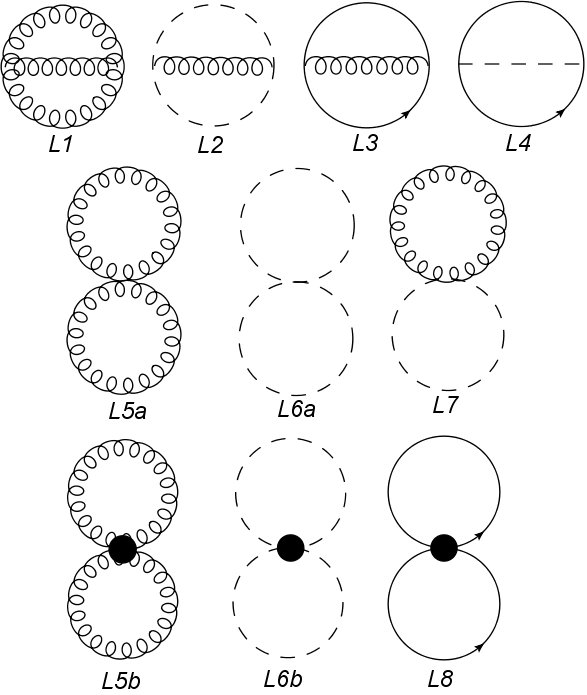
Refer to caption
Figure 4: The 2-loop diagrams obtained after integrating cc and aa. Vertices with a little circle correspond to terms we got after integrating the linear aa vertex.

Diagrams 𝐋𝟏\mathbf{L_{1}}, 𝐋𝟓​𝐚\mathbf{L_{5a}} and 𝐋𝟓​𝐛\mathbf{L_{5b}} were already evaluated in [9]. The expressions for the other diagrams that contribute in the planar limit are,

𝐋𝟐\displaystyle\mathbf{L_{2}} =−2βg2NsCα​β​γCα¯​β¯​γ¯∫0βdtΔβi​j(t)Δαj​k(t)Δγk​i(t),\displaystyle=-2\beta g^{2}N_{s}C^{\alpha\beta\gamma}C^{\bar{\alpha}\bar{\beta}\bar{\gamma}}\int_{0}^{\beta}dt\Delta_{\beta}^{ij}(t)\Delta_{\alpha}^{jk}(t)\Delta_{\gamma}^{ki}(t), (4.1.1)
𝐋𝟑\displaystyle\mathbf{L_{3}} =12βg2NfGα​β​γGβ​α​γ¯∫0βdt{Θαi​j(−t)Θβi​k(t)Δγk​j(t)+\displaystyle=\frac{1}{2}\beta g^{2}N_{f}G^{\alpha\beta\gamma}G^{\beta\alpha\bar{\gamma}}\int_{0}^{\beta}dt\left\{\Theta_{\alpha}^{ij}(-t)\Theta_{\beta}^{ik}(t)\Delta_{\gamma}^{kj}(t)+\right.
+Θαi​j(−t)Θβk​j(t)Δγi​k(t)},\displaystyle~~~\left.+\Theta_{\alpha}^{ij}(-t)\Theta_{\beta}^{kj}(t)\Delta_{\gamma}^{ik}(t)\right\}, (4.1.2)
𝐋𝟒\displaystyle\mathbf{L_{4}} =−12βg2tr(ρa†ρa)Fα¯​β​γFα​β¯​γ¯∫0βdt{Θαi​j(t)Δγj​k(t)Θβk​i(t)+Θαi​j(t)Δγk​i(t)Θβj​k(t)},\displaystyle=-\frac{1}{2}\beta g^{2}\mathrm{tr}(\rho^{a{\dagger}}\rho^{a})F^{\bar{\alpha}\beta\gamma}F^{\alpha\bar{\beta}\bar{\gamma}}\int_{0}^{\beta}dt\left\{\Theta_{\alpha}^{ij}(t)\Delta_{\gamma}^{jk}(t)\Theta_{\beta}^{ki}(t)+\Theta_{\alpha}^{ij}(t)\Delta_{\gamma}^{ki}(t)\Theta_{\beta}^{jk}(t)\right\}, (4.1.3)
𝐋𝟔​𝐚\displaystyle\mathbf{L_{6a}} =−14​β​g2​𝐐a​a​b​b​(Bα​α¯​γ​Bβ​β¯​γ¯+Bα​β​γ​Bα¯​β¯​γ¯)​Δαi​j​(0)​Δβj​k​(0),\displaystyle=-\frac{1}{4}\beta g^{2}\mathbf{Q}^{aabb}\left(B^{\alpha\bar{\alpha}\gamma}B^{\beta\bar{\beta}\bar{\gamma}}+B^{\alpha\beta\gamma}B^{\bar{\alpha}\bar{\beta}\bar{\gamma}}\right)\Delta^{ij}_{\alpha}(0)\Delta^{jk}_{\beta}(0), (4.1.4)
𝐋𝟔​𝐛\displaystyle\mathbf{L_{6b}} =β​g2​Ns​Bα​β​γ​Bα¯​β¯​γ¯jγ​(jγ+2)​(Dτ​Δαi​j​(0)​Dτ​Δβi​k​(0)+(jβ+1)2​Δαi​j​(0)​Δβj​k​(0)),\displaystyle=\beta g^{2}N_{s}\frac{B^{\alpha\beta\gamma}B^{\bar{\alpha}\bar{\beta}\bar{\gamma}}}{j_{\gamma}(j_{\gamma}+2)}\left(D_{\tau}\Delta^{ij}_{\alpha}(0)D_{\tau}\Delta^{ik}_{\beta}(0)+(j_{\beta}+1)^{2}\Delta^{ij}_{\alpha}(0)\Delta^{jk}_{\beta}(0)\right), (4.1.5)
𝐋𝟕\displaystyle\mathbf{L_{7}} =β​g2​Ns​Dα​α¯​γ​Bβ​β¯​γ¯​Δαi​j​(0)​Δβj​k​(0),\displaystyle=\beta g^{2}N_{s}D^{\alpha\bar{\alpha}\gamma}B^{\beta\bar{\beta}\bar{\gamma}}\Delta^{ij}_{\alpha}(0)\Delta^{jk}_{\beta}(0), (4.1.6)
𝐋𝟖\displaystyle\mathbf{L_{8}} =β​g2​Nf​Fα​β​γ​Fβ​α​γ¯2​jγ​(jγ+2)​(Θαi​j​(0)​Θβi​k​(0)+Θαi​j​(0)​Θβk​j​(0)).\displaystyle=\beta g^{2}N_{f}\frac{F^{\alpha\beta\gamma}F^{\beta\alpha\bar{\gamma}}}{2j_{\gamma}(j_{\gamma}+2)}\left(\Theta^{ij}_{\alpha}(0)\Theta^{ik}_{\beta}(0)+\Theta^{ij}_{\alpha}(0)\Theta^{kj}_{\beta}(0)\right). (4.1.7)

Each diagram has three index loops, and the short-hand indexing on the propagators indicates how a term in their expansion in powers of ei​β​α⊗e−i​β​αe^{i\beta\alpha}\otimes e^{-i\beta\alpha} should be grouped into traces. The notation Δi​j\Delta^{ij} means that the left side of the tensor product in the expansion belongs to the index loop ii and the right side to the index loop jj. Also, the propagators above should be understood to be multiplied by the appropriate regulators.

We can sum analytically over all angular momentum quantum numbers, except the total angular momentum, by using the identities derived in appendix C.3. We then have to expand the propagators in powers of ei​β​α⊗e−i​β​αe^{i\beta\alpha}\otimes e^{-i\beta\alpha} and extract the coefficients fn​(x)f_{n}(x) and fn​m​(x)f_{nm}(x) defined in (1.2.5). The results are expressed as sums over the total angular momentum numbers constrained by some selection rules from the integrals over 3 spherical harmonics.

In all diagrams we find that we can write fn​(x)=f1,+​(xn)+(−1)n+1​f1,−​(xn)f_{n}(x)=f_{1,+}(x^{n})+(-1)^{n+1}f_{1,-}(x^{n}). The expressions for those are long and not very illuminating. They are summarized in appendix E.

4.2 Counterterm vacuum diagrams

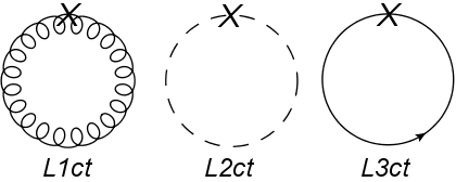
The counterterm diagrams which contribute to our computation are depicted in figure 5. For the gauge field and scalar we find that fnc​t​(x)=f1c​t​(xn)≡fc​t​(xn)f_{n}^{ct}(x)=f_{1}^{ct}(x^{n})\equiv f^{ct}(x^{n}). After summation over angular momentum we obtain1919 19 In deriving these expressions we have used the equation of motion of the propagator to determine the coefficient of Z2Z_{2}, e.g. in the bosonic case (−Dt2+(j+1)2)​Δ​(t)=δ⁡(t)(-D_{t}^{2}+(j+1)^{2})\Delta(t)=\delta(t). In principle we should have added the δ⁡(0)\delta(0) term but this term cancels with the corresponding diagram which involves the U⁡(1)U(1) part of the fields.

fgc​t​(x)=2​(Z0​g​f​(x)+(Z1​g−Z2​g)​g1​(x)),\displaystyle f_{g}^{ct}(x)=2\left(Z_{0g}f(x)+(Z_{1g}-Z_{2g})g_{1}(x)\right), (4.2.1)
fsc​t​(x)=(k⁡(x)​Z0​sa​a+g1​(x)​Z1​sa​a−(g1​(x)+k⁡(x))​Z2​sa​a),f_{s}^{ct}(x)=\left(k(x)Z^{aa}_{0s}+g_{1}(x)Z^{aa}_{1s}-\left(g_{1}(x)+k(x)\right)Z_{2s}^{aa}\right), (4.2.2)

where,

k⁡(x)=x(1−x)2,\displaystyle k(x)=\frac{x}{(1-x)^{2}},~ f⁡(x)=k⁡(x)+ln⁡(1−x),\displaystyle~f(x)=k(x)+\ln(1-x), g1​(x)=6​k​(x)2.\displaystyle g_{1}(x)=6k(x)^{2}. (4.2.3)

For the fermion we find fnc​t​(x)=(−1)n−1​f1c​t​(xn)f_{n}^{ct}(x)=(-1)^{n-1}f_{1}^{ct}(x^{n}). After summation over angular momentum we obtain,

ffc​t​(x)=6​x32​(1+x)(1−x)4​(Z1​fI​I−Z2​fI​I).f_{f}^{ct}(x)=6\frac{x^{\frac{3}{2}}(1+x)}{(1-x)^{4}}\left(Z_{1f}^{II}-Z_{2f}^{II}\right). (4.2.4)
Refer to caption
Figure 5: Counterterm vacuum diagrams which contribute to the 2-loop computation.

Plugging in the expressions for the counterterm coefficients we have computed (3.1.31)-(3.1.36), (3.2.27)-(3.2.28) we obtain,

fgc​t​(x)\displaystyle f_{g}^{ct}(x) =f(x){M2[43𝒞2200−4𝒞2100+23Ns𝒞2020−2Ns𝒞2010+83Nf𝒞2002]−\displaystyle=f(x)\left\{M^{2}\left[\frac{4}{3}\mathcal{C}_{2}^{200}-4\mathcal{C}_{2}^{100}+\frac{2}{3}N_{s}\mathcal{C}_{2}^{020}-2N_{s}\mathcal{C}_{2}^{010}+\frac{8}{3}N_{f}\mathcal{C}_{2}^{002}\right]-\right.
−115[8ℱ2g+4ℱ2s+12ℱ2f]+715​π2ln(𝒜100𝒜200)+1π2[59+2​Ns45−Nf180]}+\displaystyle\left.-\frac{1}{15}\left[8\mathcal{F}_{2}^{g}+4\mathcal{F}_{2}^{s}+12\mathcal{F}_{2}^{f}\right]+\frac{7}{15\pi^{2}}\ln\left(\frac{\mathcal{A}_{100}}{\mathcal{A}_{200}}\right)+\frac{1}{\pi^{2}}\left[\frac{5}{9}+\frac{2N_{s}}{45}-\frac{N_{f}}{180}\right]\right\}+
+g1​(x)​{115​[2​ℱ2g+Ns​ℱ2s+8​Nf​ℱ2f]+815​π2​ln⁡(𝒜200𝒜100)+30−3​Ns−14​Nf120​π2},\displaystyle+g_{1}(x)\left\{\frac{1}{15}\left[2\mathcal{F}_{2}^{g}+N_{s}\mathcal{F}_{2}^{s}+8N_{f}\mathcal{F}_{2}^{f}\right]+\frac{8}{15\pi^{2}}\ln\left(\frac{\mathcal{A}_{200}}{\mathcal{A}_{100}}\right)+\frac{30-3N_{s}-14N_{f}}{120\pi^{2}}\right\}, (4.2.5)
fsc​t​(x)\displaystyle f_{s}^{ct}(x) =k(x){M2[Qa​a​b​b𝒞2010−Ns(𝒞2010+2𝒞2100)+2tr(ρ†ρ)𝒞2002]+Ns2​π2ln(𝒜100𝒜010)+\displaystyle=k(x)\bigg\{M^{2}\left[Q^{aabb}\mathcal{C}_{2}^{010}-N_{s}\left(\mathcal{C}_{2}^{010}+2\mathcal{C}_{2}^{100}\right)+2\text{tr}(\rho^{\dagger}\rho)\mathcal{C}_{2}^{002}\right]+\frac{N_{s}}{2\pi^{2}}\ln\left(\frac{\mathcal{A}_{100}}{\mathcal{A}_{010}}\right)+
+1π2[NsC1+2tr(ρa†ρa)C2+2𝐐a​a​b​bC3)]}+\displaystyle+\frac{1}{\pi^{2}}\left[N_{s}C_{1}+2\text{tr}(\rho^{a{\dagger}}\rho^{a})C_{2}+2\mathbf{Q}^{aabb}C_{3})\right]\bigg\}+
+g1​(x)​{13​tr​(ρ†​ρ)​ℱ2f+Ns3​π2​ln⁡(𝒜110𝒜010)+Ns−tr​(ρ†​ρ)24​π2},\displaystyle+g_{1}(x)\left\{\frac{1}{3}\text{tr}(\rho^{\dagger}\rho)\mathcal{F}_{2}^{f}+\frac{N_{s}}{3\pi^{2}}\ln\left(\frac{\mathcal{A}_{110}}{\mathcal{A}_{010}}\right)+\frac{N_{s}-\text{tr}(\rho^{\dagger}\rho)}{24\pi^{2}}\right\}, (4.2.6)
ffc​t​(x)\displaystyle f_{f}^{ct}(x) =−6​x32​(1+x)(1−x)4​{Nf3​π​ℬ1g+tr​(ρ†​ρ)6​π​ℬ1s+Nf3​π2​ln⁡(𝒜001𝒜101)+−2​Nf+tr​(ρ†​ρ)24​π2}.\displaystyle=-6\frac{x^{\frac{3}{2}}(1+x)}{(1-x)^{4}}\left\{\frac{N_{f}}{3\pi}\mathcal{B}_{1}^{g}+\frac{\text{tr}(\rho^{\dagger}\rho)}{6\pi}\mathcal{B}_{1}^{s}+\frac{N_{f}}{3\pi^{2}}\ln\left(\frac{\mathcal{A}_{001}}{\mathcal{A}_{101}}\right)+\frac{-2N_{f}+\text{tr}(\rho^{\dagger}\rho)}{24\pi^{2}}\right\}. (4.2.7)

In principle we are done and all we have to do is to plug the expressions for fnf_{n} and fn​mf_{nm} we found (E.1.1)-(E.1.13), (E.2.3)-(E.2.12) summed with the counterterm expressions, (4.2.5)-(4.2.7) inside the partition function formula (1.2.11) and perform the angular momentum summations numerically.

However our regularization involved several subtleties, and it is useful to check explicitly that all regulator dependence cancels between the counterterm vacuum diagrams and the 2-loop vacuum diagrams.

In order to see this cancelation we first extract the regulator dependent part of the 2-loop diagrams by expanding asymptotically in large angular momentum as was done in [9]. The expressions we found for the regulator dependent part of each 2-loop diagram are listed in appendix E.3. One can readily check that indeed fgc​t+fsc​t+∑ifLi,+r​e​gf^{ct}_{g}+f^{ct}_{s}+\sum_{i}f^{reg}_{L_{i},+} and ffc​t+∑ifLi,−r​e​gf^{ct}_{f}+\sum_{i}f^{reg}_{L_{i},-} are regulator independent. This is a useful intermediate self consistency check on our computation.

4.3 Numerical evaluation and checks

As explained in the introduction there are two immediate applications to our calculation. One involves computing the order λ\lambda correction to the Hagedorn temperature (1.2.12) of the theory. The second involves computing the order λ\lambda corrections to the spectrum of the theory on S3S^{3}, (1.2.13).

Both have already been computed for the 𝒩=4\mathcal{N}=4 SYM case in [10] by using spin-chain methods. Their result for the small temperature expansion is2020 20 The 𝒩=4\mathcal{N}=4 partition function in (4.3.1) is adopted to our conventions. Our coupling constant is defined to be twice the one in [10].,

𝒵𝐒𝐘𝐌​(x)=1+(21+3​λ​ln⁡(x)2​π2)​x2+(96+24​λ​ln⁡(x)π2)​x5/2+(376+192​λ​ln⁡(x)π2)​x3++(1344+1032​λ​ln⁡(x)π2)​x7/2+(4836+4440​λ​ln⁡(x)π2)​x4++(17472+17712​λ​ln⁡(x)π2)​x9/2+(64608+71508​λ​ln⁡(x)π2)​x5++432​(560+341​λ​ln⁡(x)π2)​x11/2+(906741+2430477​λ​ln⁡(x)2​π2)​x6+⋯,\begin{split}\mathcal{Z}_{\mathbf{SYM}}(x)&=1+\left(21+\frac{3\lambda\ln(x)}{2\pi^{2}}\right)x^{2}+\left(96+\frac{24\lambda\ln(x)}{\pi^{2}}\right)x^{5/2}+\left(376+\frac{192\lambda\ln(x)}{\pi^{2}}\right)x^{3}+\\ &+\left(1344+\frac{1032\lambda\ln(x)}{\pi^{2}}\right)x^{7/2}+\left(4836+\frac{4440\lambda\ln(x)}{\pi^{2}}\right)x^{4}+\\ &+\left(17472+\frac{17712\lambda\ln(x)}{\pi^{2}}\right)x^{9/2}+\left(64608+\frac{71508\lambda\ln(x)}{\pi^{2}}\right)x^{5}+\\ &+432\left(560+\frac{341\lambda\ln(x)}{\pi^{2}}\right)x^{11/2}+\left(906741+\frac{2430477\lambda\ln(x)}{2\pi^{2}}\right)x^{6}+\cdots,\end{split} (4.3.1)

while the correction to the Hagedorn temperature is,

δ​xH=−xH​λ​ln⁡(xH)4​π2.\displaystyle\delta x_{H}=-x_{H}\frac{\lambda\ln(x_{H})}{4\pi^{2}}. (4.3.2)

Using our computation method we can perform this expansion and compute the perturbative correction to the Hagedorn temperature numerically. As a self consistency check we indeed found that the numerics do not depend on the choice of regulating function.

However before we compare our computation to (4.3.1) and (4.3.2), we must fix the arbitrary constant piece in (4.2.6). Recall that the source of the constants C1C_{1}, C2C_{2} and C3C_{3} in fsc​t​(x)f_{s}^{ct}(x) is the mass renormalization of the scalar fields (3.2.28). Since a mass term for the scalars is gauge invariant, these constants are arbitrary. In particular to order x2x^{2} our computation yields the following partition function,

𝒵⁡(x)\displaystyle\mathcal{Z}(x) =1+[Ns​(Ns+1)2+λ​ln⁡(x)48​π2((Ns+1)(Ns(48C1−33)+(96C2+11)tr(ρa†ρa)+\displaystyle=1+\bigg[\frac{N_{s}(N_{s}+1)}{2}+\frac{\lambda\ln(x)}{48\pi^{2}}\big(\left(N_{s}+1\right)\left(N_{s}(48C_{1}-33)+(96C_{2}+11)\mathrm{tr}(\rho^{a{\dagger}}\rho^{a})+\right.
+(96C3+1)𝐐a​a​b​b)+6𝐐a​a​b​b)]x2+⋯.\displaystyle+\left.(96C_{3}+1)\mathbf{Q}^{aabb}\right)+6\mathbf{Q}^{aabb}\big)\bigg]x^{2}+\cdots. (4.3.3)

If our theory is conformally invariant to order λ\lambda, then the coefficient of xn​ln⁡(x)x^{n}\ln(x) in (4.3.3) is the sum of the anomalous dimensions of operators with classical dimension nn in the flat space theory (see below (1.2.13)). In particular, the operators of dimension 2 are,

𝒪^2a​b≡tr⁡(ϕa​ϕb).\displaystyle\hat{\mathcal{O}}_{2}^{ab}\equiv\mathrm{tr}(\phi^{a}\phi^{b}). (4.3.4)

We computed the anomalous dimension matrix of those operators in the flat space theory corresponding to (2.1.1)2121 21 The assumption of having only commutator interactions is implicit in (4.3.5) since only the combination 𝐐a​a​b​b\mathbf{Q}^{aabb} appears in it. Under this assumption the two possible combinations are related by 𝐐a​b​a​b=−12​𝐐a​a​b​b\mathbf{Q}^{abab}=-\frac{1}{2}\mathbf{Q}^{aabb}.,

∑dim⁡[𝒪^]=2γ𝒪^\displaystyle\sum_{\mathrm{dim}\left[\hat{\mathcal{O}}\right]=2}\gamma_{\hat{\mathcal{O}}} =−λ8​π2[3Ns(Ns+1)−(Ns+1)tr(ρa†ρa)−𝐐a​a​b​b],\displaystyle=-\frac{\lambda}{8\pi^{2}}\left[3N_{s}(N_{s}+1)-(N_{s}+1)\mathrm{tr}(\rho^{a{\dagger}}\rho^{a})-\mathbf{Q}^{aabb}\right], (4.3.5)

Comparing the coefficient of the x2​ln⁡(x)x^{2}\ln(x) in (4.3.3) to (4.3.5) we can solve for C1C_{1}, C2C_{2} and C3C_{3},

C1=516,C2=−596,C3=−196.\displaystyle C_{1}=\frac{5}{16},~~C_{2}=-\frac{5}{96},~~C_{3}=-\frac{1}{96}. (4.3.6)

We evaluated the angular momentum sums in the 2-loop diagrams numerically up to order x6x^{6} (we could easily have reached higher orders with more computer time but it was not needed in this work),

f1,+​(x)\displaystyle f_{1,+}(x) ≡∑if1,+L​i​(x)+fgc​t​(x)+fsc​t​(x)=\displaystyle\equiv\sum_{i}f_{1,+}^{Li}(x)+f^{ct}_{g}(x)+f^{ct}_{s}(x)=
=1π2[(−38Ns+18tr(ρa†ρa))x+\displaystyle=\frac{1}{\pi^{2}}\left[\left(-\frac{3}{8}N_{s}+\frac{1}{8}\mathrm{tr}(\rho^{a{\dagger}}\rho^{a})\right)x\right.+
+(14+12Nf+18Ns−18𝐐a​b​b​a+12tr(ρa†ρa))x2+\displaystyle+\left(\frac{1}{4}+\frac{1}{2}N_{f}+\frac{1}{8}N_{s}-\frac{1}{8}\mathbf{Q}^{abba}+\frac{1}{2}\mathrm{tr}(\rho^{a{\dagger}}\rho^{a})\right)x^{2}+
+(4+2Nf+258Ns−12𝐐a​b​b​a+118tr(ρa†ρa))x3+\displaystyle+\left(4+2N_{f}+\frac{25}{8}N_{s}-\frac{1}{2}\mathbf{Q}^{abba}+\frac{11}{8}\mathrm{tr}(\rho^{a{\dagger}}\rho^{a})\right)x^{3}+
+(554+5Nf+414Ns−54𝐐a​b​b​a+3tr(ρa†ρa))x4+\displaystyle+\left(\frac{55}{4}+5N_{f}+\frac{41}{4}N_{s}-\frac{5}{4}\mathbf{Q}^{abba}+3\mathrm{tr}(\rho^{a{\dagger}}\rho^{a})\right)x^{4}+
+(32+10Nf+1858Ns−52𝐐a​b​b​a+458tr(ρa†ρa))x5+\displaystyle+\left(32+10N_{f}+\frac{185}{8}N_{s}-\frac{5}{2}\mathbf{Q}^{abba}+\frac{45}{8}\mathrm{tr}(\rho^{a{\dagger}}\rho^{a})\right)x^{5}+
+(2454+352Nf+3478Ns−358𝐐a​b​b​a+192tr(ρa†ρa))x6+⋯],\displaystyle\left.+\left(\frac{245}{4}+\frac{35}{2}N_{f}+\frac{347}{8}N_{s}-\frac{35}{8}\mathbf{Q}^{abba}+\frac{19}{2}\mathrm{tr}(\rho^{a{\dagger}}\rho^{a})\right)x^{6}+\cdots\right], (4.3.7)
f1−​(x)\displaystyle f_{1-}(x) ≡∑if1,−L​i​(x)+ffc​t​(x)=\displaystyle\equiv\sum_{i}f_{1,-}^{Li}(x)+f^{ct}_{f}(x)=
=1π2[14tr(ρa†ρa)x32+(3Nf+54tr(ρa†ρa))x52+\displaystyle=\frac{1}{\pi^{2}}\left[\frac{1}{4}\mathrm{tr}(\rho^{a{\dagger}}\rho^{a})x^{\frac{3}{2}}+(3N_{f}+\frac{5}{4}\mathrm{tr}(\rho^{a{\dagger}}\rho^{a}))x^{\frac{5}{2}}+\right.
+(12Nf+72tr(ρa†ρa))x72+(30Nf+152tr(ρa†ρa))x92+\displaystyle+(12N_{f}+\frac{7}{2}\mathrm{tr}(\rho^{a{\dagger}}\rho^{a}))x^{\frac{7}{2}}+(30N_{f}+\frac{15}{2}\mathrm{tr}(\rho^{a{\dagger}}\rho^{a}))x^{\frac{9}{2}}+
+(60Nf+554tr(ρa†ρa))x112+⋯],\displaystyle\left.+(60N_{f}+\frac{55}{4}\mathrm{tr}(\rho^{a{\dagger}}\rho^{a}))x^{\frac{11}{2}}+\cdots\right], (4.3.8)
F~2n​p​(x)\displaystyle\widetilde{F}_{2}^{np}(x) ≡∑iF~2,L​in​p=\displaystyle\equiv\sum_{i}\widetilde{F}_{2,Li}^{np}=
=𝐐a​a​b​b8​π2​x2−tr(ρa†ρa)π2​x52+\displaystyle=\frac{\mathbf{Q}^{aabb}}{8\pi^{2}}x^{2}-\frac{\mathrm{tr}(\rho^{a{\dagger}}\rho^{a})}{\pi^{2}}x^{\frac{5}{2}}+
+[4𝐐a​a​b​b−2tr(ρa†ρa)−6Nf−9Ns]4​π2​x3−4tr(ρa†ρa)π2​x72+\displaystyle+\frac{\left[4\mathbf{Q}^{aabb}\!-\!2\mathrm{tr}(\rho^{a{\dagger}}\rho^{a})\!-\!6N_{f}\!-\!9N_{s}\right]}{4\pi^{2}}x^{3}\!-\!\frac{4\mathrm{tr}(\rho^{a{\dagger}}\rho^{a})}{\pi^{2}}x^{\frac{7}{2}}+
++23​𝐐a​a​b​b−48​Ns8​π2​x4+3(Nf−3tr(ρa†ρa))π2​x92+\displaystyle+\frac{18\!+\!23\mathbf{Q}^{aabb}\!-\!48N_{s}}{8\pi^{2}}x^{4}\!+\!\frac{3(N_{f}\!-3\mathrm{tr}(\rho^{a{\dagger}}\rho^{a}))}{\pi^{2}}x^{\frac{9}{2}}+
+14𝐐a​a​b​b−tr(ρa†ρa)−9Nf−39Ns2​π2​x5−20tr(ρa†ρa)π2​x112+\displaystyle+\!\frac{\!14\mathbf{Q}^{aabb}\!-\!\mathrm{tr}(\rho^{a{\dagger}}\rho^{a})\!-9N_{f}-\!39N_{s}}{2\pi^{2}}x^{5}-\frac{20\mathrm{tr}(\rho^{a{\dagger}}\rho^{a})}{\pi^{2}}x^{\frac{11}{2}}+
+42+50𝐐a​a​b​b−6tr(ρa†ρa)−18Nf−117Ns4​π2​x6+⋯.\displaystyle+\frac{42+50\mathbf{Q}^{aabb}-6\mathrm{tr}(\rho^{a{\dagger}}\rho^{a})-18N_{f}-117N_{s}}{4\pi^{2}}x^{6}+\cdots. (4.3.9)

One can plug those in (1.2.11) and see that for 𝒩=4\mathcal{N}=4 (see appendix A) we reproduce (4.3.1) and (4.3.2). This is a very non-trivial check of our computation.

It is also important to have a check for the generic theory which is not conformally invariant, in order to make sure that conformal invariance is preserved to order λ\lambda by our renormalization scheme. To do so we computed the anomalous dimensions of dimension 5/2 and 3 operators,

𝒪^52I​a\displaystyle\hat{\mathcal{O}}^{Ia}_{\frac{5}{2}} ≡tr⁡(ψI​ϕa),\displaystyle\equiv\mathrm{tr}(\psi^{I}\phi^{a}), 𝒪^3a​μ​ν\displaystyle\hat{\mathcal{O}}_{3}^{a\mu\nu} ≡i​tr​(ϕa​Fμ​ν),\displaystyle\equiv i\mathrm{tr}(\phi^{a}F^{\mu\nu}), 𝒪^3I​α​J​β\displaystyle\hat{\mathcal{O}}_{3}^{I\alpha J\beta} ≡tr⁡(ψαI​ψβJ)\displaystyle\equiv\mathrm{tr}(\psi^{I}_{\alpha}\psi^{J}_{\beta})
𝒪^3a​b​c\displaystyle\hat{\mathcal{O}}_{3}^{abc} ≡tr⁡(ϕa​ϕb​ϕc),\displaystyle\equiv\mathrm{tr}(\phi^{a}\phi^{b}\phi^{c}), 𝒪^31​a​b\displaystyle\hat{\mathcal{O}}_{3}^{1ab} ≡i​∂μtr⁡(ϕa​ϕb),\displaystyle\equiv i\partial_{\mu}\mathrm{tr}(\phi^{a}\phi^{b}), 𝒪^32​a​b\displaystyle\hat{\mathcal{O}}_{3}^{2ab} ≡itr(ϕ[aDμϕb]),\displaystyle\equiv i\mathrm{tr}(\phi^{[a}D_{\mu}\phi^{b]}), (4.3.10)

for which we found,

∑dim⁡[𝒪^]=5/2γ𝒪^\displaystyle\sum_{\mathrm{dim}\left[\hat{\mathcal{O}}\right]=5/2}\gamma_{\hat{\mathcal{O}}} =−λ4​π2(6NsNf+tr(ρaρa†)(4−Ns−2Nf))\displaystyle=-\frac{\lambda}{4\pi^{2}}\left(6N_{s}N_{f}+\mathrm{tr}(\rho^{a}\rho^{a{\dagger}})(4-N_{s}-2N_{f})\right) (4.3.11)
∑dim⁡[𝒪^]=3γ𝒪^\displaystyle\sum_{\mathrm{dim}\left[\hat{\mathcal{O}}\right]=3}\gamma_{\hat{\mathcal{O}}} =λπ2(−5Ns−118Ns2−38Ns3−32Nf+12NsNf+14tr(ρa†ρa)+Nstr(ρa†ρa)+\displaystyle=\frac{\lambda}{\pi^{2}}\left(-5N_{s}-\frac{11}{8}N_{s}^{2}-\frac{3}{8}N_{s}^{3}-\frac{3}{2}N_{f}+\frac{1}{2}N_{s}N_{f}+\frac{1}{4}\mathrm{tr}(\rho^{a{\dagger}}\rho^{a})+N_{s}\mathrm{tr}(\rho^{a{\dagger}}\rho^{a})+\right.
+Nftr(ρa†ρa)+18Ns2tr(ρa†ρa)+𝐐a​a​b​b−18Ns𝐐a​a​b​b),\displaystyle\left.+N_{f}\mathrm{tr}(\rho^{a{\dagger}}\rho^{a})+\frac{1}{8}N_{s}^{2}\mathrm{tr}(\rho^{a{\dagger}}\rho^{a})+\mathbf{Q}^{aabb}-\frac{1}{8}N_{s}\mathbf{Q}^{aabb}\right), (4.3.12)

in agreement with the results derived from (4.3.7)-(4.3.9). This gives a check that by applying our renormalization scheme for the scalar field mass terms, the general theory is indeed conformally invariant to order λ\lambda.

In the pure YM and 𝒩=4\mathcal{N}=4 SYM theories Δ​TH≡π2​δ​TH/TH\Delta T_{H}\equiv\pi^{2}\delta T_{H}/T_{H} was found to be positive and rational. In the more general cases that we considered, we found that this quantity can be either positive or negative and that it is not necessarily rational. For example, consider gauge theories with Ns+Nf=10N_{s}+N_{f}=10, 𝐐a​a​b​b=Ns​(1−Ns)\mathbf{Q}^{aabb}=N_{s}(1-N_{s}) corresponding to tr​([ϕa,ϕb]2)\text{tr}([\phi^{a},\phi^{b}]^{2}) self interaction, and tr(ρaρa†)=NsNf\text{tr}(\rho^{a}\rho^{a{\dagger}})=N_{s}N_{f} Yukawa couplings. Strangely, it turns out that all these theories have xH​(λ=0)=7−4​3x_{H}(\lambda=0)=7-4\sqrt{3}. The results for Δ​TH\Delta T_{H} for these theories are,

NsN_{s} 1010 99 88 77 66
NfN_{f} 00 11 22 33 44
Δ​TH\Delta T_{H} −1/8-1/8 0.0170450.017045 1/81/8 0.2017860.201786 1/41/4

For pure scalar theories with the same self interactions as above, Δ​TH\Delta T_{H} becomes negative for Ns>2N_{s}>2 but is not necessarily rational. For instance,

NsN_{s} 1010 1111 1212 1313 1414 1515 1616 1717 1818 1919 2020
Δ​TH\Delta T_{H} −18-\frac{1}{8} −0.132353-0.132353 −536-\frac{5}{36} −0.144737-0.144737 −320-\frac{3}{20} −0.154762-0.154762 −744-\frac{7}{44} −0.163043-0.163043 −16-\frac{1}{6} −17100-\frac{17}{100} −0.173077-0.173077

For generic couplings the results are of course irrational, but as we see in the examples above, rational results are not so difficult to construct. It would be interesting to understand the reason for Δ​TH\Delta T_{H} to be rational.

5 Conclusions

In this work we have computed the full large NN partition function of S​U​(N)SU(N) YM theory on S3S^{3} in perturbation theory, to 2-loops order. We included scalar and spinor fields in the adjoint representation of the gauge group, with arbitrary commutator interactions. The computation involved expanding those fields in Kaluza-Klein modes on S3S^{3}. Then, instead of solving momentum integrals, we had to perform sums over the angular momentum of those modes and derive various identities in order to perform these sums. Furthermore, we used a cutoff regularization scheme which is not gauge invariant. To deal with this we added non-gauge invariant counterterms to the theory and demanded that their value precisely compensates for the non-gauge invariance introduced by the regulator.

Furthermore, we demanded that our theory is conformally invariant to order λ\lambda, so that we can relate the perturbative corrections to the energy spectrum on S3×ℝS^{3}\times\mathds{R}, to the sums of anomalous dimensions on ℝ4\mathds{R}^{4}, by using the state-operator mapping. Though generically our theories have a non-zero beta function, it contributes to the partition function only at higher orders. The only obstruction to achieving conformal invariance at order λ\lambda is the generation of mass terms for the scalar fields. By demanding that the state-operator mapping works for dimension 2 operators, we can fix the mass renormalization of the scalar fields such that the theory is still conformal at order λ\lambda.

Our computation agrees with known results for the 1-loop anomalous dimensions of 𝒩=4\mathcal{N}=4 SYM which were computed in [10]. This is a highly non-trivial check on our computation which was done by a very different method. Our results can be used to numerically compute the partition function in the confinement phase of the large NN gauge theories which we considered. Furthermore, the order λ\lambda correction to the Hagedorn temperature can be computed very easily for those theories.

This computation also has a direct application towards determining the order of the deconfinement phase transition. As shown in [6] this involves a 3-loop computation, and the 2-loop computation of f11​(x)f_{11}(x). The latter can be computed from our results for the fn​mL​i​(x)f_{nm}^{Li}(x)’s (E.2.3)-(E.2.12).

Acknowledgments

We would like to thank Ofer Aharony for suggesting this work as an M.Sc project, and for his help and guidance throughout. We would also like to thank Mark Van Raamsdonk for comments on a draft of this paper. This work was supported in part by the Israel-U.S. Binational Science Foundation, by a center of excellence supported by the Israel Science Foundation (grant number 1468/06), by a grant (DIP H52) of the German Israel Project Cooperation, by the European network MRTN-CT-2004-512194, and by Minerva.

Appendix A Additional notations

Having enough indices as it is in our computation, we use matrix notation for spinors. Our notation for the Weyl spinor matrices is such that,

σμ≡(1,i​τi),\displaystyle\sigma^{\mu}\equiv(1,i\tau^{i})~~,~~ σ¯μ≡(1,−i​τi),\displaystyle\bar{\sigma}^{\mu}\equiv(1,-i\tau^{i}), (A.0.1)

where τi\tau^{i} are the usual Pauli matrices. Also we use the charge conjugation matrix in the Yukawa terms,

ε≡i​τ2.\displaystyle\varepsilon\equiv i\tau^{2}. (A.0.2)

In order to apply our computation to 𝒩=4\mathcal{N}=4 SYM, take Ns=6N_{s}=6 and Nf=4N_{f}=4. Furthermore, in that case the Yukawa matrices satisfy,

ρa†ρb+ρb†ρa=2δa​b𝟙4×4,\displaystyle\rho^{a{\dagger}}\rho^{b}+\rho^{b{\dagger}}\rho^{a}=2\delta^{ab}\mathds{1}_{4\times 4}, (A.0.3)

while the quartic scalar coupling satisfies,

𝐐a​b​c​d=2​δa​c​δb​d−δa​d​δc​b−δa​b​δd​c.\displaystyle\mathbf{Q}^{abcd}=2\delta^{ac}\delta^{bd}-\delta^{ad}\delta^{cb}-\delta^{ab}\delta^{dc}. (A.0.4)

Appendix B The gauge fixed Yang-Mills action on S3S^{3}

B.1 The action

Imposing the gauge conditions (1.2.1), (1.2.2) and adding the conformal coupling for the scalar fields, the Euclidean action on S3S^{3} can be written as 𝐒E=𝐒g+𝐒s+𝐒f\mathbf{S}_{E}=\mathbf{S}_{g}+\mathbf{S}_{s}+\mathbf{S}_{f} where,

𝐒g\displaystyle\mathbf{S}_{g} =∫0βdt∫S3tr{−12Ai(Dt2+∂j2)Ai−12A0∂2A0−c†∂2c+\displaystyle=\int_{0}^{\beta}dt\int_{S^{3}}\textrm{tr}\left\{-\frac{1}{2}A_{i}(D_{t}^{2}+\partial_{j}^{2})A^{i}-\frac{1}{2}A_{0}\partial^{2}A_{0}-c^{{\dagger}}\partial^{2}c+\right.
+i​g​Dt​Ai​[Ai,A0]−i​g​[Ai,A0]​∂iA0−i​g​∂iAj​[Ai,Aj]+\displaystyle+igD_{t}A^{i}[A_{i},A_{0}]-ig[A^{i},A_{0}]\partial_{i}A_{0}-ig\partial_{i}A_{j}[A^{i},A^{j}]+ (B.1.1)
+14g2[Ai,Aj][Aj,Ai]−12g2[A0,Ai][A0,Ai]−ig∂ic†[Ai,c]},\displaystyle\left.+\frac{1}{4}g^{2}[A_{i},A_{j}][A^{j},A^{i}]-\frac{1}{2}g^{2}[A_{0},A_{i}][A^{0},A^{i}]-ig\partial_{i}c^{{\dagger}}[A_{i},c]\right\},

where we define Dt≡∂t−[α,∗]D_{t}\equiv\partial_{t}-[\alpha,*]. For the pure conformally coupled scalar (kinetic plus quartic interaction),

𝐒s=\displaystyle\mathbf{S}_{s}= ∫0βdt∫S3tr{−12Φa(Dt2+∂i2−1)Φa−\displaystyle\int_{0}^{\beta}dt\int_{S^{3}}\textrm{tr}\left\{-\frac{1}{2}\Phi_{a}(D_{t}^{2}+\partial_{i}^{2}-1)\Phi_{a}-\right.
−i​g​[A0,Φa]​Dt​Φa−i​g​[Ai,Φa]​∂iΦa\displaystyle-ig[A_{0},\Phi_{a}]D_{t}\Phi_{a}-ig[A_{i},\Phi_{a}]\partial^{i}\Phi_{a} (B.1.2)
−12g2[Ai,Φa]2−12g2[A0,Φa]2−14g2𝐐a​b​c​dΦaΦbΦcΦd},\displaystyle\left.-\frac{1}{2}g^{2}[A_{i},\Phi_{a}]^{2}-\frac{1}{2}g^{2}[A_{0},\Phi_{a}]^{2}-\frac{1}{4}g^{2}\mathbf{Q}^{abcd}\Phi_{a}\Phi_{b}\Phi_{c}\Phi_{d}\right\},

and for the fermions (kinetic plus Yukawa interaction) we write,

𝐒f\displaystyle\mathbf{S}_{f} =∫0βdt∫S3tr{iΨ†I(Dt+σi∂i)ΨI+\displaystyle=\int_{0}^{\beta}dt\int_{S^{3}}\textrm{tr}\left\{i\Psi^{{\dagger}I}(D_{t}+\sigma^{i}\partial_{i})\Psi_{I}+\right.
+gΨ†I[A0,ΨI]+gΨI†σi[Ai,ΨI]+\displaystyle+g\Psi^{{\dagger}I}[A_{0},\Psi_{I}]+g\Psi^{I{\dagger}}\sigma^{i}[A_{i},\Psi_{I}]+ (B.1.3)
+12gΨITε(ρa†)I​J[Φa,ΨJ]+12gΨ†IερI​Ja[Φa,(Ψ†J)T]}.\displaystyle\left.+\frac{1}{2}g\Psi_{I}^{T}\varepsilon(\rho^{a{\dagger}})^{IJ}[\Phi_{a},\Psi_{J}]+\frac{1}{2}g\Psi^{{\dagger}I}\varepsilon\rho^{a}_{IJ}[\Phi_{a},(\Psi^{{\dagger}J})^{T}]\right\}.

In the above the spatial derivative is assumed to be the covariant one on S3S^{3} including the appropriate connection terms for vectors and spinors.

Using the properties listed in appendix C we can write the action in terms of the expansions of the fields in Kaluza-Klein modes (2.1.4), and in terms of the spherical harmonics integrals (2.1.5) as 𝐒E=𝐒2+𝐒3+𝐒4\mathbf{S}_{E}=\mathbf{S}_{2}+\mathbf{S}_{3}+\mathbf{S}_{4}, with

𝐒2\displaystyle\mathbf{S}_{2} =∫0βdttr{12Aα¯(−Dt2+(jα+1)2)Aα+12aα¯jα(jα+2)aα+c†αjα(jα+2)cα+\displaystyle=\int_{0}^{\beta}dt\mathrm{tr}\left\{\frac{1}{2}A^{\bar{\alpha}}(-D_{t}^{2}+(j_{\alpha}+1)^{2})A^{\alpha}+\frac{1}{2}a^{\bar{\alpha}}j_{\alpha}(j_{\alpha}+2)a^{\alpha}+c^{{\dagger}\alpha}j_{\alpha}(j_{\alpha}+2)c^{\alpha}+\right.
+12ϕaα¯(−Dt2+(jα+1)2)ϕaα+iψ†α​I(Dt+ϵα(jα+12))ψIα}.\displaystyle~\left.+\frac{1}{2}\phi_{a}^{\bar{\alpha}}(-D_{t}^{2}+(j_{\alpha}+1)^{2})\phi_{a}^{\alpha}+i\psi^{{\dagger}\alpha I}(D_{t}+\epsilon_{\alpha}(j_{\alpha}+\frac{1}{2}))\psi^{\alpha}_{I}\right\}. (B.1.4)
𝐒3\displaystyle\mathbf{S}_{3} =ig∫0βdttr{Cα¯​β​γc†α[Aβ,cγ]+2Cα​β​γaαAβaγ−\displaystyle=ig\int_{0}^{\beta}dt\mathrm{tr}\bigg\{C^{\bar{\alpha}\beta\gamma}c^{{\dagger}\alpha}[A^{\beta},c^{\gamma}]+2C^{\alpha\beta\gamma}a^{\alpha}A^{\beta}a^{\gamma}-
−Dα​β​γ​[Aα,Dt​Aβ]​aγ+ϵα​(jα+1)​Eα​β​γ​Aα​Aβ​Aγ−Bα​β​γ​[aα,ϕaβ]​Dt​ϕaγ−\displaystyle~-D^{\alpha\beta\gamma}[A^{\alpha},D_{t}A^{\beta}]a^{\gamma}+\epsilon_{\alpha}(j_{\alpha}+1)E^{\alpha\beta\gamma}A^{\alpha}A^{\beta}A^{\gamma}-B^{\alpha\beta\gamma}[a^{\alpha},\phi^{\beta}_{a}]D_{t}\phi_{a}^{\gamma}-
−Cα​β​γ​[Aβ,ϕaα]​ϕaγ−i​Fα​β​γ​ψ†α​I​[aγ,ψIβ]−i​Gα​β​γ​ψ†α​I​[Aγ,ψIβ]−\displaystyle~-C^{\alpha\beta\gamma}[A^{\beta},\phi_{a}^{\alpha}]\phi_{a}^{\gamma}-iF^{\alpha\beta\gamma}\psi^{{\dagger}\alpha I}[a^{\gamma},\psi_{I}^{\beta}]-iG^{\alpha\beta\gamma}\psi^{{\dagger}\alpha I}[A^{\gamma},\psi^{\beta}_{I}]-
−i2Fα¯​β​γψIα(ρa†)I​J[ϕaγ,ψJβ]+i2Fα​β¯​γψ†I​αρI​Ja[ϕaγ,ψ†J​β]}.\displaystyle~\left.-\frac{i}{2}F^{\bar{\alpha}\beta\gamma}\psi_{I}^{\alpha}(\rho^{a{\dagger}})^{IJ}[\phi_{a}^{\gamma},\psi_{J}^{\beta}]+\frac{i}{2}F^{\alpha\bar{\beta}\gamma}\psi^{{\dagger}I\alpha}\rho^{a}_{IJ}[\phi_{a}^{\gamma},\psi^{{\dagger}J\beta}]\right\}. (B.1.5)
𝐒4\displaystyle\mathbf{S}_{4} =−12g2∫0βdttr{(Dβ​λ¯​αDδ​λ​γ+1jλ​(jλ+2)Cα​β​λ¯Cγ​δ​λ)[aα,Aβ][aγ,Aδ]+\displaystyle=-\frac{1}{2}g^{2}\int_{0}^{\beta}dt\mathrm{tr}\left\{\left(D^{\beta\bar{\lambda}\alpha}D^{\delta\lambda\gamma}+\frac{1}{j_{\lambda}(j_{\lambda}+2)}C^{\alpha\beta\bar{\lambda}}C^{\gamma\delta\lambda}\right)[a^{\alpha},A^{\beta}][a^{\gamma},A^{\delta}]+\right.
+(Dα​γ​λ¯​Dβ​δ​λ−Dα​δ​λ¯​Dβ​γ​λ)​Aα​Aβ​Aγ​Aδ+Bα​β​λ¯​Bλ​γ​δ​[aα,ϕaβ]​[aγ,ϕaδ]+\displaystyle~+\left(D^{\alpha\gamma\bar{\lambda}}D^{\beta\delta\lambda}-D^{\alpha\delta\bar{\lambda}}D^{\beta\gamma\lambda}\right)A^{\alpha}A^{\beta}A^{\gamma}A^{\delta}+B^{\alpha\beta\bar{\lambda}}B^{\lambda\gamma\delta}[a^{\alpha},\phi_{a}^{\beta}][a^{\gamma},\phi_{a}^{\delta}]+
+Dα​γ​λBλ¯​β​δ[Aα,ϕaβ][Aγ,ϕaδ]+12Bα​β​λ¯Bλ​γ​δ𝐐a​b​c​dϕaαϕbβϕcγϕdδ}.\displaystyle~\left.+D^{\alpha\gamma\lambda}B^{\bar{\lambda}\beta\delta}[A^{\alpha},\phi_{a}^{\beta}][A^{\gamma},\phi_{a}^{\delta}]+\frac{1}{2}B^{\alpha\beta\bar{\lambda}}B^{\lambda\gamma\delta}\mathbf{Q}^{abcd}\phi_{a}^{\alpha}\phi_{b}^{\beta}\phi_{c}^{\gamma}\phi_{d}^{\delta}\right\}. (B.1.6)

B.2 Integrating out aa and cc

The fields aa and cc appear only quadratically in the gauge fixed action (B.1.4)-(B.1.6) and it is convenient to integrate them out first. Their propagators are,

⟨ci​jα​(t′)​ck​l†β​(t)⟩\displaystyle\langle c^{\alpha}_{ij}(t^{\prime})c^{{\dagger}\beta}_{kl}(t)\rangle =1jα​(jα+2)​δ​(t′−t)​δα​β​δi​l​δk​j,\displaystyle=\frac{1}{j_{\alpha}(j_{\alpha}+2)}\delta(t^{\prime}-t)\delta^{\alpha\beta}\delta_{il}\delta_{kj}, (B.2.1)
⟨ai​jα(t′)ak​lβ(t)\displaystyle\langle a^{\alpha}_{ij}(t^{\prime})a^{\beta}_{kl}(t) =1jα​(jα+2)​δ​(t′−t)​δα​β¯​δi​l​δk​j.\displaystyle=\frac{1}{j_{\alpha}(j_{\alpha}+2)}\delta(t^{\prime}-t)\delta^{\alpha\bar{\beta}}\delta_{il}\delta_{kj}. (B.2.2)

From loops of aa’s and cc’s we get the effective vertices,

A2A\displaystyle A_{2}^{A} =N​g2​Dβ​λ¯​α​Dδ​λ​α¯jα​(jα+2)​∫0βd​t​δ​(0)​tr​(Aβ​Aδ)\displaystyle=Ng^{2}\frac{D^{\beta\bar{\lambda}\alpha}D^{\delta\lambda\bar{\alpha}}}{j_{\alpha}(j_{\alpha}+2)}\int_{0}^{\beta}dt\delta(0)\textrm{tr}(A^{\beta}A^{\delta}) (B.2.3)
A2ϕ\displaystyle A_{2}^{\phi} =N​g2​Bα​β​λ¯​Bα¯​δ​λjα​(jα+2)​∫0βd​t​δ​(0)​tr​(ϕaβ​ϕaδ).\displaystyle=Ng^{2}\frac{B^{\alpha\beta\bar{\lambda}}B^{\bar{\alpha}\delta\lambda}}{j_{\alpha}(j_{\alpha}+2)}\int_{0}^{\beta}dt\delta(0)\textrm{tr}(\phi^{\beta}_{a}\phi^{\delta}_{a}). (B.2.4)

The other diagrams arise from strings of aa’s using the linear aa vertices in (B.1.5),

B4A\displaystyle B^{A}_{4} =g22​Dα​β​λ​Dγ​δ​λ¯jλ​(jλ+2)​∫0βd​t​tr​([Aα,Dτ​Aβ]​[Aγ,Dτ​Aδ]),\displaystyle=\frac{g^{2}}{2}\frac{D^{\alpha\beta\lambda}D^{\gamma\delta\bar{\lambda}}}{j_{\lambda}(j_{\lambda}+2)}\int^{\beta}_{0}dt\mathrm{tr}\left([A^{\alpha},D_{\tau}A^{\beta}][A^{\gamma},D_{\tau}A^{\delta}]\right), (B.2.5)
B4ϕ\displaystyle B^{\phi}_{4} =g22​Bα​β​λ​Bγ​δ​λ¯jλ​(jλ+2)​∫0βd​t​tr​([ϕaα,Dτ​ϕaβ]​[ϕbγ,Dτ​ϕbδ]),\displaystyle=\frac{g^{2}}{2}\frac{B^{\alpha\beta\lambda}B^{\gamma\delta\bar{\lambda}}}{j_{\lambda}(j_{\lambda}+2)}\int^{\beta}_{0}dt\mathrm{tr}\left([\phi^{\alpha}_{a},D_{\tau}\phi^{\beta}_{a}][\phi^{\gamma}_{b},D_{\tau}\phi_{b}^{\delta}]\right), (B.2.6)
B4ψ\displaystyle B^{\psi}_{4} =−g22Fα​β​λ​Fγ​δ​λ¯jλ​(jλ+2)∫0βdttr({ψIβ,ψ†α​I}{ψJδ,ψ†γ​J}),\displaystyle=-\frac{g^{2}}{2}\frac{F^{\alpha\beta\lambda}F^{\gamma\delta\bar{\lambda}}}{j_{\lambda}(j_{\lambda}+2)}\int^{\beta}_{0}dt\textrm{tr}\left(\{\psi^{\beta}_{I},\psi^{\dagger\alpha I}\}\{\psi_{J}^{\delta},\psi^{\dagger\gamma J}\}\right), (B.2.7)
B2,2A​ϕ\displaystyle B^{A\phi}_{2,2} =g2​Dα​β​λ​Bγ​δ​λ¯jλ​(jλ+2)​∫0βd​t​tr​([Aα,Dτ​Aβ]​[ϕaγ,Dτ​ϕaδ]),\displaystyle=g^{2}\frac{D^{\alpha\beta\lambda}B^{\gamma\delta\bar{\lambda}}}{j_{\lambda}(j_{\lambda}+2)}\int^{\beta}_{0}dt\mathrm{tr}\left([A^{\alpha},D_{\tau}A^{\beta}][\phi^{\gamma}_{a},D_{\tau}\phi^{\delta}_{a}]\right), (B.2.8)
B2,2A​ψ\displaystyle B^{A\psi}_{2,2} =i​g2​Dα​β​λ​Fγ​δ​λ¯jλ​(jλ+2)​∫0βd​t​tr​([Aα,Dτ​Aβ]​{ψIδ,ψ†γ​I}),\displaystyle=ig^{2}\frac{D^{\alpha\beta\lambda}F^{\gamma\delta\bar{\lambda}}}{j_{\lambda}(j_{\lambda}+2)}\int^{\beta}_{0}dt\mathrm{tr}\left([A^{\alpha},D_{\tau}A^{\beta}]\{\psi_{I}^{\delta},\psi^{\dagger\gamma I}\}\right), (B.2.9)
B2,2ϕ​ψ\displaystyle B^{\phi\psi}_{2,2} =i​g2​Bα​β​λ​Fγ​δ​λ¯jλ​(jλ+2)​∫0βd​t​tr​([ϕaα,Dτ​ϕaβ]​{ψIδ,ψ†γ​I}).\displaystyle=ig^{2}\frac{B^{\alpha\beta\lambda}F^{\gamma\delta\bar{\lambda}}}{j_{\lambda}(j_{\lambda}+2)}\int^{\beta}_{0}dt\mathrm{tr}\left([\phi_{a}^{\alpha},D_{\tau}\phi_{a}^{\beta}]\{\psi_{I}^{\delta},\psi^{\dagger\gamma I}\}\right). (B.2.10)

The δ⁡(0)\delta(0) divergence in (B.2.3) and (B.2.4) is an artifact of the Coulomb gauge and arises since aa and cc are not dynamical fields. We see that those vertices cancel by adding to them the expressions obtained by contracting the two covariant derivatives, in (B.2.5) and (B.2.6) (see (2.2)). Therefore we can forget about δ⁡(0)\delta(0) factors for diagrams which involve those vertices.

Also the vacuum diagrams which arise from one insertion of any of the vertices (B.2.8), (B.2.9) or (B.2.10) vanish for kinematical reasons. After the self contractions the summation over spherical harmonics (see (C.3.4), (C.3.7) ,(C.3.8)) vanishes unless jλ=0j_{\lambda}=0, which can not be since this is the angular momenta of aλa^{\lambda}, (A0A_{0}) whose zero mode has been factored out.

Appendix C Properties of S3S^{3} spherical harmonics

C.1 S3S^{3} spherical harmonics

In this section we list some properties of spherical harmonics that we used. Due to lack of space this is far from a complete review, and the interested reader is referred to [8], [13] for scalar and vector spherical harmonics, and to [14],[15] for spinor spherical harmonics.

Spherical harmonics sit in representations of the isometry group of S3S^{3}, which is S​O​(4)≃S​U​(2)×S​U​(2)SO(4)\simeq SU(2)\times SU(2). The scalar spherical harmonics transform in the (j/2,j/2)(j/2,j/2) representation, where j≥0j\geq 0 and −j/2≤m,m′≤j/2-j/2\leq m,m^{\prime}\leq j/2.

They form a complete orthonormal set of eigenfunctions of the corresponding laplacian on S3S^{3},

∇2𝒮jm,n=−j⁡(j+2)​𝒮jm,n,\nabla^{2}\mathcal{S}^{m,n}_{j}=-j(j+2)\mathcal{S}^{m,n}_{j}, (C.1.1)

and satisfy the conjugation relation,

(𝒮jm,n)∗\displaystyle(\mathcal{S}^{m,n}_{j})^{*} =(−1)m+n​𝒮j−m,−n.\displaystyle=(-1)^{m+n}\mathcal{S}^{-m,-n}_{j}. (C.1.2)

The vector spherical harmonics sit in the ((j+ϵ)/2,(j−ϵ)/2)((j+\epsilon)/2,(j-\epsilon)/2) representation, where ϵ=±1\epsilon=\pm 1 and j≥1j\geq 1. This set of functions satisfies the eigenvalue equations,

∇2𝒱→j,ϵm,n=−(j+1)2​𝒱→j,ϵm,n,∇→×𝒱→j,ϵm,n=−ϵ⁡(j+1)​𝒱→j,ϵm,n,∇→⋅𝒱→j,ϵm,n=0,\displaystyle\begin{array}[]{lll}\nabla^{2}\vec{\mathcal{V}}^{m,n}_{j,\epsilon}&=&-(j+1)^{2}\vec{\mathcal{V}}^{m,n}_{j,\epsilon},\\ \vec{\nabla}\times\vec{\mathcal{V}}^{m,n}_{j,\epsilon}&=&-\epsilon(j+1)\vec{\mathcal{V}}^{m,n}_{j,\epsilon},\\ \vec{\nabla}\cdot\vec{\mathcal{V}}^{m,n}_{j,\epsilon}&=&0,\end{array}

and the conjugation relation,

(𝒱→j,ϵm,n)∗\displaystyle(\vec{\mathcal{V}}^{m,n}_{j,\epsilon})^{*} =(−1)m+n+1​𝒱→j,ϵ−m,−n.\displaystyle=(-1)^{m+n+1}\vec{\mathcal{V}}^{-m,-n}_{j,\epsilon}. (C.1.7)

The spinor spherical harmonics are two-component Weyl spinors, and transform in the representations (j−(1−ϵ)/22,j−(1+ϵ)/22)(\frac{j-(1-\epsilon)/2}{2},\frac{j-(1+\epsilon)/2}{2}) for ϵ=±1\epsilon=\pm 1 and j≥1j\geq 1. They can be found from the scalar functions by tensor multiplying a (j/2,j/2)(j/2,j/2) representation, with a (1/2,0)(1/2,0), (or (0,1/2)(0,1/2)) basis spinor with the right Clebsch-Gordan coefficients. The properly normalized result is

𝒴j,+m,n=1j​(j/2+m​𝒮j−1m−1/2,nj/2−m​𝒮j−1m+1/2,n),𝒴j,−m,n=1j+1​(−j/2−m+1/2​𝒮jm−1/2,nj/2+m+1/2​𝒮jm+1/2,n).\displaystyle\begin{array}[]{lll}\mathcal{Y}^{m,n}_{j,+}&=&~~~\frac{1}{\sqrt{j}}\begin{pmatrix}\sqrt{j/2+m}\mathcal{S}^{m-1/2,n}_{j-1}\\ \sqrt{j/2-m}\mathcal{S}^{m+1/2,n}_{j-1}\end{pmatrix},\\ \mathcal{Y}^{m,n}_{j,-}&=&\frac{1}{\sqrt{j+1}}\begin{pmatrix}-\sqrt{j/2-m+1/2}\mathcal{S}^{m-1/2,n}_{j}\\ \sqrt{j/2+m+1/2}\mathcal{S}^{m+1/2,n}_{j}\end{pmatrix}.\par\end{array}

From the properties of the scalar functions one can check that those are normalized correctly

∫S3𝒴m,n†j,ϵ𝒴m′,n′j′,ϵ′=δj,j′δm,m′δn,n′δϵ,ϵ′,\int_{S^{3}}\mathcal{Y}^{m,n{\dagger}}_{j,\epsilon}\mathcal{Y}^{m^{\prime},n^{\prime}}_{j^{\prime},\epsilon^{\prime}}=\delta_{j,j^{\prime}}\delta_{m,m^{\prime}}\delta_{n,n^{\prime}}\delta_{\epsilon,\epsilon^{\prime}}, (C.1.11)

and that under conjugation those obey

(𝒴j,ϵm,n)∗=(−1)m+n−ϵ/2​ε​(𝒴j,ϵ−m,−n).\left(\mathcal{Y}^{m,n}_{j,\epsilon}\right)^{*}=(-1)^{m+n-\epsilon/2}\varepsilon\left(\mathcal{Y}^{-m,-n}_{j,\epsilon}\right). (C.1.12)

The spinor functions satisfy the eigenvalues equation2222 22 The inclusion of the appropriate veilbein and spin connection should be understood. Also recall that in our convention for spinor matrices the σi\sigma^{i} are anti-hermitian, hence the real eigenvalue in the above equation.,

σi​∂i𝒴j,ϵm,n=ϵ⁡(j+12)​𝒴j,ϵm,n.\displaystyle\sigma^{i}\partial_{i}\mathcal{Y}^{m,n}_{j,\epsilon}=\epsilon(j+\frac{1}{2})\mathcal{Y}^{m,n}_{j,\epsilon}. (C.1.13)

In the text we collect all the angular momentum indices of a scalar, vector or spinor spherical harmonic by a single Greek index. A barred Greek index on a scalar or vector spherical harmonic means the corresponding function is conjugated, while by a barred Greek index on a spinor spherical harmonic we mean 𝒴α¯≡(−1)mα+nα−ϵα/2​(𝒴jα,ϵα−mα,−nα)\mathcal{Y}^{\bar{\alpha}}\equiv(-1)^{m_{\alpha}+n_{\alpha}-\epsilon_{\alpha}/2}\left(\mathcal{Y}^{-m_{\alpha},-n_{\alpha}}_{j_{\alpha},\epsilon_{\alpha}}\right).

C.2 Spherical harmonics integrals

While expanding our fields in Kaluza-Klein modes on S3S^{3} we defined integrals over three spherical harmonics (2.1.5). These integrals can be expressed as a reduced matrix element times the appropriate 3-j symbols,

Bα​β​γ\displaystyle B^{\alpha\beta\gamma} =RB​(jα,jβ,jγ)​(jα2jβ2jγ2mαmβmγ)​(jα2jβ2jγ2nαnβnγ),\displaystyle=R_{B}(j_{\alpha},j_{\beta},j_{\gamma})\begin{pmatrix}\frac{j_{\alpha}}{2}&\frac{j_{\beta}}{2}&\frac{j_{\gamma}}{2}\\ m_{\alpha}&m_{\beta}&m_{\gamma}\end{pmatrix}\begin{pmatrix}\frac{j_{\alpha}}{2}&\frac{j_{\beta}}{2}&\frac{j_{\gamma}}{2}\\ n_{\alpha}&n_{\beta}&n_{\gamma}\end{pmatrix},
Cα​β​γ\displaystyle C^{{\alpha}{\beta}{\gamma}} =RC​(jα,jβ,jγ)​(jα2jβ+ϵβ2jγ2mαmβmγ)​(jα2jβ−ϵβ2jγ2nαnβnγ),\displaystyle=R_{C}(j_{\alpha},j_{\beta},j_{\gamma})\begin{pmatrix}\frac{j_{\alpha}}{2}&\frac{j_{\beta}+\epsilon_{\beta}}{2}&\frac{j_{\gamma}}{2}\\ m_{\alpha}&m_{\beta}&m_{\gamma}\end{pmatrix}\begin{pmatrix}\frac{j_{\alpha}}{2}&\frac{j_{\beta}-\epsilon_{\beta}}{2}&\frac{j_{\gamma}}{2}\\ n_{\alpha}&n_{\beta}&n_{\gamma}\end{pmatrix},
Dα​β​γ\displaystyle D^{{\alpha}{\beta}{\gamma}} =RD​ϵα​ϵβ​(jα,jβ,jγ)​(jα+ϵα2jβ+ϵβ2jγ2mαmβmγ)​(jα−ϵα2jβ−ϵβ2jγ2nαnβnγ),\displaystyle=R_{D\epsilon_{\alpha}\epsilon_{\beta}}(j_{\alpha},j_{\beta},j_{\gamma})\begin{pmatrix}\frac{j_{\alpha}+\epsilon_{\alpha}}{2}&\frac{j_{\beta}+\epsilon_{\beta}}{2}&\frac{j_{\gamma}}{2}\\ m_{\alpha}&m_{\beta}&m_{\gamma}\end{pmatrix}\begin{pmatrix}\frac{j_{\alpha}-\epsilon_{\alpha}}{2}&\frac{j_{\beta}-\epsilon_{\beta}}{2}&\frac{j_{\gamma}}{2}\\ n_{\alpha}&n_{\beta}&n_{\gamma}\end{pmatrix}, (C.2.1)
Eα​β​γ\displaystyle E^{{\alpha}{\beta}{\gamma}} =RE​ϵα​ϵβ​ϵγ​(jα,jβ,jγ)​(jα+ϵα2jβ+ϵβ2jγ+ϵγ2mαmβmγ)​(jα−ϵα2jβ−ϵβ2jγ−ϵγ2nαnβnγ),\displaystyle=R_{E\epsilon_{\alpha}\epsilon_{\beta}\epsilon_{\gamma}}(j_{\alpha},j_{\beta},j_{\gamma})\begin{pmatrix}\frac{j_{\alpha}+\epsilon_{\alpha}}{2}&\frac{j_{\beta}+\epsilon_{\beta}}{2}&\frac{j_{\gamma}+\epsilon_{\gamma}}{2}\\ m_{\alpha}&m_{\beta}&m_{\gamma}\end{pmatrix}\begin{pmatrix}\frac{j_{\alpha}-\epsilon_{\alpha}}{2}&\frac{j_{\beta}-\epsilon_{\beta}}{2}&\frac{j_{\gamma}-\epsilon_{\gamma}}{2}\\ n_{\alpha}&n_{\beta}&n_{\gamma}\end{pmatrix},
Hα​β​γ\displaystyle H^{{\alpha}{\beta}{\gamma}} =RH​ϵα​ϵβ​(jα,jβ,jγ)​((jα−(1−ϵα)/2)2(jβ−(1−ϵβ)/2)2jγ2mαmβmγ)​((jα−(1+ϵα)/2)2(jβ−(1+ϵβ)/2)2jγ2nαnβnγ),\displaystyle=R_{H\epsilon_{\alpha}\epsilon_{\beta}}(j_{\alpha},j_{\beta},j_{\gamma})\begin{pmatrix}\frac{(j_{\alpha}-(1-\epsilon_{\alpha})/2)}{2}&\frac{(j_{\beta}-(1-\epsilon_{\beta})/2)}{2}&\frac{j_{\gamma}}{2}\\ m_{\alpha}&m_{\beta}&m_{\gamma}\end{pmatrix}\begin{pmatrix}\frac{(j_{\alpha}-(1+\epsilon_{\alpha})/2)}{2}&\frac{(j_{\beta}-(1+\epsilon_{\beta})/2)}{2}&\frac{j_{\gamma}}{2}\\ n_{\alpha}&n_{\beta}&n_{\gamma}\end{pmatrix},
G~α​β​γ\displaystyle\tilde{G}^{{\alpha}{\beta}{\gamma}} =RG~​ϵα​ϵβ​ϵγ​(jα,jβ,jγ)​((jα−(1−ϵα)/2)2(jβ−(1−ϵβ)/2)2jγ+ϵγ2mαmβmγ)​((jα−(1+ϵα)/2)2(jβ−(1+ϵβ)/2)2jγ−ϵγ2nαnβnγ).\displaystyle=R_{\tilde{G}\epsilon_{\alpha}\epsilon_{\beta}\epsilon_{\gamma}}(j_{\alpha},j_{\beta},j_{\gamma})\begin{pmatrix}\frac{(j_{\alpha}-(1-\epsilon_{\alpha})/2)}{2}&\frac{(j_{\beta}-(1-\epsilon_{\beta})/2)}{2}&\frac{j_{\gamma}+\epsilon_{\gamma}}{2}\\ m_{\alpha}&m_{\beta}&m_{\gamma}\end{pmatrix}\begin{pmatrix}\frac{(j_{\alpha}-(1+\epsilon_{\alpha})/2)}{2}&\frac{(j_{\beta}-(1+\epsilon_{\beta})/2)}{2}&\frac{j_{\gamma}-\epsilon_{\gamma}}{2}\\ n_{\alpha}&n_{\beta}&n_{\gamma}\end{pmatrix}.

where,

G~α​β​γ=∫d​Ω​(𝒴α)T​ε​σi​𝒴β​𝒱iγ.\tilde{G}^{{\alpha}{\beta}{\gamma}}=\int d\Omega(\mathcal{Y}^{{\alpha}})^{T}\varepsilon\sigma^{i}\mathcal{Y}^{{\beta}}\mathcal{V}_{i}^{\gamma}. (C.2.2)

This can be related to the fermionic integrals listed in (2.1.5), by using the conjugation relations of the spinor spherical functions (C.1.12).

We computed the reduced matrix elements which were not already evaluated in [8] explicitly,

RH+​(x,y,z)\displaystyle R_{H+}(x,y,z) =\displaystyle= (−1)σ+1π​[(z+1)​(σ−z)​(σ+1)2]12,\displaystyle\frac{(-1)^{\sigma+1}}{\pi}\left[\frac{(z+1)(\sigma-z)(\sigma+1)}{2}\right]^{\frac{1}{2}},
RH−​(x,y,z)\displaystyle R_{H-}(x,y,z) =\displaystyle= (−1)σ~+1π​[(z+1)​(σ~−x)​(σ~−y)2]12,\displaystyle\frac{(-1)^{\tilde{\sigma}+1}}{\pi}\left[\frac{(z+1)(\tilde{\sigma}-x)(\tilde{\sigma}-y)}{2}\right]^{\frac{1}{2}},
RG~​0​(x,y,z)\displaystyle R_{\tilde{G}0}(x,y,z) =\displaystyle= (−1)σ~+1π​[(σ~−x)​(σ~−y)​σ~​(σ~+1)(z+1)]12,\displaystyle\frac{(-1)^{\tilde{\sigma}+1}}{\pi}\left[\frac{(\tilde{\sigma}-x)(\tilde{\sigma}-y)\tilde{\sigma}(\tilde{\sigma}+1)}{(z+1)}\right]^{\frac{1}{2}}, (C.2.3)
RG~​1​(x,y,z)\displaystyle R_{\tilde{G}1}(x,y,z) =\displaystyle= (−1)σ~+1π​[(σ~−x)​(σ~−y)​(σ~−z−1)​(σ~−z)(z+1)]12,\displaystyle\frac{(-1)^{\tilde{\sigma}+1}}{\pi}\left[\frac{(\tilde{\sigma}-x)(\tilde{\sigma}-y)(\tilde{\sigma}-z-1)(\tilde{\sigma}-z)}{(z+1)}\right]^{\frac{1}{2}},
RG~​2​(x,y,z)\displaystyle R_{\tilde{G}2}(x,y,z) =\displaystyle= (−1)σπ​[(σ−z)​(σ+1)​(σ−y)​(σ−y+1)(z+1)]12,\displaystyle\frac{(-1)^{\sigma}}{\pi}\left[\frac{(\sigma-z)(\sigma+1)(\sigma-y)(\sigma-y+1)}{(z+1)}\right]^{\frac{1}{2}},

where σ≡(x+y+z)/2\sigma\equiv(x+y+z)/2 and σ~≡(x+y+z+1)/2\tilde{\sigma}\equiv(x+y+z+1)/2 are integers and,

RH+≡RH++=RH−−,\displaystyle R_{H+}\equiv R_{H++}=R_{H--},~ RH−≡RH+−=−RH−+,\displaystyle~R_{H-}\equiv R_{H+-}=-R_{H-+},
RG~​0≡RG~+++=RG~−−−,\displaystyle R_{\tilde{G}0}\equiv R_{\tilde{G}+++}=R_{\tilde{G}---},~ RG~​1≡RG~−−+=−RG~++−,\displaystyle~R_{\tilde{G}1}\equiv R_{\tilde{G}--+}=-R_{\tilde{G}++-}, (C.2.4)
RG~​2≡RG~+−+=RG~−+−,\displaystyle R_{\tilde{G}2}\equiv R_{\tilde{G}+-+}=R_{\tilde{G}-+-},~ RG~​2​(x↔y)=−RG~−++=−RG~+−−.\displaystyle~R_{\tilde{G}2}(x\leftrightarrow y)=-R_{\tilde{G}-++}=-R_{\tilde{G}+--}.

C.3 Performing angular momentum sums

We computed various sums over spherical harmonics quantum numbers, which appear in the expressions for our diagrams. We list those identities which were not already derived in [9]2323 23 Translating the notation in [9] to ours: R2→RCR_{2}\rightarrow R_{C} , R3​ϵα​ϵβ→RD​ϵα​ϵβR_{3\epsilon_{\alpha}\epsilon_{\beta}}\rightarrow R_{D\epsilon_{\alpha}\epsilon_{\beta}}, and R4​ϵα​ϵβ​ϵγ→RE​ϵα​ϵβ​ϵγR_{4\epsilon_{\alpha}\epsilon_{\beta}\epsilon_{\gamma}}\rightarrow R_{E\epsilon_{\alpha}\epsilon_{\beta}\epsilon_{\gamma}}. ,

∑m′​sGα​β​γ​Gβ​α​γ¯\displaystyle\sum_{m^{\prime}s}G^{\alpha\beta\gamma}G^{\beta\alpha\bar{\gamma}} =(−1)ϵα+ϵβ2​RG~​ϵα​ϵβ​ϵγ​(jα,jβ,jγ)​RG~​ϵβ​ϵα​ϵγ​(jβ,jα,jγ),\displaystyle=(-1)^{\frac{\epsilon_{\alpha}+\epsilon_{\beta}}{2}}R_{\tilde{G}\epsilon_{\alpha}\epsilon_{\beta}\epsilon_{\gamma}}(j_{\alpha},j_{\beta},j_{\gamma})R_{\tilde{G}\epsilon_{\beta}\epsilon_{\alpha}\epsilon_{\gamma}}(j_{\beta},j_{\alpha},j_{\gamma}), (C.3.1)
∑m′​sFα¯​β​γ​Fα​β¯​γ¯\displaystyle\sum_{m^{\prime}s}F^{\bar{\alpha}\beta\gamma}F^{\alpha\bar{\beta}\bar{\gamma}} =(−1)jα+jβ+jγ+ϵα+ϵβ2​RH​ϵα​ϵβ2​(jα,jβ,jγ),\displaystyle=(-1)^{j_{\alpha}+j_{\beta}+j_{\gamma}+\frac{\epsilon_{\alpha}+\epsilon_{\beta}}{2}}R_{H\epsilon_{\alpha}\epsilon_{\beta}}^{2}(j_{\alpha},j_{\beta},j_{\gamma}), (C.3.2)
∑m′​sBα​β​γ​Bα¯​β¯​γ¯\displaystyle\sum_{m^{\prime}s}B^{\alpha\beta\gamma}B^{\bar{\alpha}\bar{\beta}\bar{\gamma}} =RB2​(jα,jβ,jγ),\displaystyle=R_{B}^{2}(j_{\alpha},j_{\beta},j_{\gamma}), (C.3.3)
∑m′​s,ϵ′​sDα​α¯​γ​Bβ​β¯​γ¯\displaystyle\sum_{m^{\prime}s,\epsilon^{\prime}s}D^{\alpha\bar{\alpha}\gamma}B^{\beta\bar{\beta}\bar{\gamma}} =2(−1)jα+jβ+1δjγ,0×\displaystyle=2(-1)^{j_{\alpha}+j_{\beta}+1}\delta_{j_{\gamma},0}\times
×jα​(jα+2)​(jβ+1)​RD+​(jα,jα,0)​RB​(jβ,jβ,0),\displaystyle\times\sqrt{j_{\alpha}(j_{\alpha}+2)}(j_{\beta}+1)R_{D+}(j_{\alpha},j_{\alpha},0)R_{B}(j_{\beta},j_{\beta},0), (C.3.4)
∑m′​sFα​β​γ​Fβ​α​γ¯\displaystyle\sum_{m^{\prime}s}F^{\alpha\beta\gamma}F^{\beta\alpha\bar{\gamma}} =(−1)1+ϵα+ϵβ2​RH​ϵα​ϵβ​(jα,jβ,jγ)​RH​ϵβ​ϵα​(jβ,jα,jγ),\displaystyle=(-1)^{1+\frac{\epsilon_{\alpha}+\epsilon_{\beta}}{2}}R_{H\epsilon_{\alpha}\epsilon_{\beta}}(j_{\alpha},j_{\beta},j_{\gamma})R_{H\epsilon_{\beta}\epsilon_{\alpha}}(j_{\beta},j_{\alpha},j_{\gamma}), (C.3.5)
∑m′​sFα​α​γ​Fβ​β​γ¯\displaystyle\sum_{m^{\prime}s}F^{\alpha\alpha\gamma}F^{\beta\beta\bar{\gamma}} =(−1)jα+jβ+jγ+1+ϵα+ϵβ2(jα(jα+1)jβ(jβ+1))12δjγ,0×\displaystyle=(-1)^{j_{\alpha}+j_{\beta}+j_{\gamma}+1+\frac{\epsilon_{\alpha}+\epsilon_{\beta}}{2}}(j_{\alpha}(j_{\alpha}+1)j_{\beta}(j_{\beta}+1))^{\frac{1}{2}}\delta_{j_{\gamma},0}\times
×RH+​(jα,jα,jγ)​RH+​(jβ,jβ,jγ),\displaystyle~~~\times R_{H+}(j_{\alpha},j_{\alpha},j_{\gamma})R_{H+}(j_{\beta},j_{\beta},j_{\gamma}), (C.3.6)
∑m′​s,ϵαDα​α¯​γ​Fβ​β​γ¯\displaystyle\sum_{m^{\prime}s,\epsilon_{\alpha}}D^{\alpha\bar{\alpha}\gamma}F^{\beta\beta\bar{\gamma}} =2(−1)jα+jβ+1+ϵβ2(jα(jα+2)jβ(jβ+1))12δjγ,0×\displaystyle=2(-1)^{j_{\alpha}+j_{\beta}+\frac{1+\epsilon_{\beta}}{2}}(j_{\alpha}(j_{\alpha}+2)j_{\beta}(j_{\beta}+1))^{\frac{1}{2}}\delta_{j_{\gamma},0}\times
×RD+​(jα,jα,jγ)​RH+​(jβ,jβ,jγ),\displaystyle~~~\times R_{D+}(j_{\alpha},j_{\alpha},j_{\gamma})R_{H+}(j_{\beta},j_{\beta},j_{\gamma}), (C.3.7)
∑m′​sBα​α¯​γ​Fβ​β​γ¯\displaystyle\sum_{m^{\prime}s}B^{\alpha\bar{\alpha}\gamma}F^{\beta\beta\bar{\gamma}} =(−1)jα+jβ+1+ϵβ2(jα+1)(jβ(jβ+1))12δjγ,0×\displaystyle=(-1)^{j_{\alpha}+j_{\beta}+\frac{1+\epsilon_{\beta}}{2}}(j_{\alpha}+1)(j_{\beta}(j_{\beta}+1))^{\frac{1}{2}}\delta_{j_{\gamma},0}\times
×RB​(jα,jα,jγ)​RH+​(jβ,jβ,jγ),\displaystyle~~~\times R_{B}(j_{\alpha},j_{\alpha},j_{\gamma})R_{H+}(j_{\beta},j_{\beta},j_{\gamma}), (C.3.8)
∑m′​s,jγBα​β​γ​Bα¯​β¯​γ¯\displaystyle\sum_{m^{\prime}s,j_{\gamma}}B^{\alpha\beta\gamma}B^{\bar{\alpha}\bar{\beta}\bar{\gamma}} =(jα+1)2​(jβ+1)22​π2.\displaystyle=\frac{(j_{\alpha}+1)^{2}(j_{\beta}+1)^{2}}{2\pi^{2}}. (C.3.9)

Appendix D 1-loop self energy diagrams

D.1 Flat space self-energy diagrams

D.1.1 Dimensional regularization

We write the flat space 1PI self-energy diagrams (figure 1) which were computed in dimensional regularization, in terms of the integrals Im,n≡Im,n​(0)I_{m,n}\equiv I_{m,n}(0) (3.1.17) ,

Vector p2p^{2} expansion: −12​⟨Ai​(0,p)​Aj​(0,−p)⟩p2​δi​j1​P​I-\frac{1}{2}\langle A_{i}(0,p)A_{j}(0,-p)\rangle^{1PI}_{p^{2}\delta_{ij}}.
𝐒𝐄𝟏𝐚\displaystyle\mathbf{SE1a} =−4​d2−22​d−20(d+3)​(d+5)​I0,2+2​d2+14​d+4(d+3)​(d+5)​I0,3−8​(2+d)(d+3)​(d+5)​I0,4,\displaystyle=\frac{-4d^{2}-22d-20}{(d+3)(d+5)}I_{0,2}+\frac{2d^{2}+14d+4}{(d+3)(d+5)}I_{0,3}-\frac{8(2+d)}{(d+3)(d+5)}I_{0,4}, (D.1.1)
𝐒𝐄𝟏𝐛\displaystyle\mathbf{SE1b} =d2+3​d−6(d+3)​(d+5)​I1,1,\displaystyle=\frac{d^{2}+3d-6}{(d+3)(d+5)}I_{1,1}, (D.1.2)
𝐒𝐄𝟏𝐜\displaystyle\mathbf{SE1c} =2​Nsd+3​[I0,3−4d+5​I0,4],\displaystyle=\frac{2N_{s}}{d+3}\left[I_{0,3}-\frac{4}{d+5}I_{0,4}\right], (D.1.3)
𝐒𝐄𝟏𝐝\displaystyle\mathbf{SE1d} =2​Nf​[I1,3−4d+3​I1,4+I0,3−4d+5​I0,4].\displaystyle=2N_{f}\left[I_{1,3}-\frac{4}{d+3}I_{1,4}+I_{0,3}-\frac{4}{d+5}I_{0,4}\right]. (D.1.4)
Vector ω2\omega^{2} expansion: −12​⟨Ai​(ω,0)​Aj​(−ω,0)⟩ω2​δi​j1​P​I-\frac{1}{2}\langle A_{i}(\omega,0)A_{j}(-\omega,0)\rangle^{1PI}_{\omega^{2}\delta_{ij}}
𝐒𝐄𝟏𝐚\displaystyle\mathbf{SE1a} =d+2d+3​[2​I0,3−8​I1,4],\displaystyle=\frac{d+2}{d+3}\left[2I_{0,3}-8I_{1,4}\right], (D.1.5)
𝐒𝐄𝟏𝐛\displaystyle\mathbf{SE1b} =−d+2d+3​I0,1,\displaystyle=-\frac{d+2}{d+3}I_{0,1}, (D.1.6)
𝐒𝐄𝟏𝐜\displaystyle\mathbf{SE1c} =2​Nsd+3​[I0,3−4​I1,4],\displaystyle=\frac{2N_{s}}{d+3}\left[I_{0,3}-4I_{1,4}\right], (D.1.7)
𝐒𝐄𝟏𝐝\displaystyle\mathbf{SE1d} =2​Nf​[d+1d+3​I0,3+3​I1,3−4​d+1d+3​I1,4−4​I2,4].\displaystyle=2N_{f}\left[\frac{d+1}{d+3}I_{0,3}+3I_{1,3}-4\frac{d+1}{d+3}I_{1,4}-4I_{2,4}\right]. (D.1.8)
Scalar p2p^{2} expansion: −12​⟨ϕa​(0,p)​ϕb​(0,−p)⟩p21​P​I-\frac{1}{2}\langle\phi^{a}(0,p)\phi^{b}(0,-p)\rangle^{1PI}_{p^{2}}.
𝐒𝐄𝟐𝐚\displaystyle\mathbf{SE2a} =−δa​b​4​(d+2)d+3​I0,2,\displaystyle=-\delta^{ab}\frac{4(d+2)}{d+3}I_{0,2}, (D.1.9)
𝐒𝐄𝟐𝐛\displaystyle\mathbf{SE2b} =δa​b​d−1d+3​I1,1,\displaystyle=\delta^{ab}\frac{d-1}{d+3}I_{1,1}, (D.1.10)
𝐒𝐄𝟐𝐜\displaystyle\mathbf{SE2c} =−tr(ρa†ρb+ρb†ρa)[−I0,2+2d+3I0,3].\displaystyle=-\mathrm{tr}(\rho^{a{\dagger}}\rho^{b}+\rho^{b{\dagger}}\rho^{a})\left[-I_{0,2}+\frac{2}{d+3}I_{0,3}\right]. (D.1.11)
Scalar ω2\omega^{2} expansion: −12​⟨ϕa​(ω,0)​ϕb​(−ω,0)⟩ω21​P​I-\frac{1}{2}\langle\phi^{a}(\omega,0)\phi^{b}(-\omega,0)\rangle^{1PI}_{\omega^{2}}.
𝐒𝐄𝟐𝐚\displaystyle\mathbf{SE2a} =0,\displaystyle=0, (D.1.12)
𝐒𝐄𝟐𝐛\displaystyle\mathbf{SE2b} =−δa​b​I0,1,\displaystyle=-\delta^{ab}I_{0,1}, (D.1.13)
𝐒𝐄𝟐𝐜\displaystyle\mathbf{SE2c} =−tr(ρa†ρb+ρb†ρa)[−I0,2+2I1,3].\displaystyle=-\mathrm{tr}(\rho^{a{\dagger}}\rho^{b}+\rho^{b{\dagger}}\rho^{a})\left[-I_{0,2}+2I_{1,3}\right]. (D.1.14)
Fermion pp expansion: ⟨ψI​(0,p)​ψ†J​(0,p)⟩pi​σi1​P​I\langle\psi_{I}(0,p)\psi^{{\dagger}J}(0,p)\rangle^{1PI}_{p_{i}\sigma^{i}}.
𝐒𝐄𝟑𝐚\displaystyle\mathbf{SE3a} =δIJ​2d+3​[−(d2+3​d+2)​I0,2+2​(d+2)​I0,3],\displaystyle=\delta_{I}^{~J}\frac{2}{d+3}\left[-(d^{2}+3d+2)I_{0,2}+2(d+2)I_{0,3}\right], (D.1.15)
𝐒𝐄𝟑𝐛\displaystyle\mathbf{SE3b} =δIJ​[−2​I0,1+4d+3​I0,2],\displaystyle=\delta_{I}^{~J}\left[-2I_{0,1}+\frac{4}{d+3}I_{0,2}\right], (D.1.16)
𝐒𝐄𝟑𝐜\displaystyle\mathbf{SE3c} =−2(ρaρa†)IJ[I0,2−2d+3I0,3].\displaystyle=-2(\rho^{a}\rho^{a{\dagger}})_{I}^{~J}\left[I_{0,2}-\frac{2}{d+3}I_{0,3}\right]. (D.1.17)
Fermion ω\omega expansion: ⟨ψI​(ω,0)​ψ†J​(ω,0)⟩ω1​P​I\langle\psi_{I}(\omega,0)\psi^{{\dagger}J}(\omega,0)\rangle^{1PI}_{\omega}.
𝐒𝐄𝟑𝐚\displaystyle\mathbf{SE3a} =δIJ​2​(d+2)​[−I0,2+2​I1,3],\displaystyle=\delta_{I}^{~J}2(d+2)\left[-I_{0,2}+2I_{1,3}\right], (D.1.18)
𝐒𝐄𝟑𝐛\displaystyle\mathbf{SE3b} =δIJ​[2​I0,1−4​I1,2]=0,\displaystyle=\delta_{I}^{~J}\left[2I_{0,1}-4I_{1,2}\right]=0, (D.1.19)
𝐒𝐄𝟑𝐜\displaystyle\mathbf{SE3c} =−2(ρaρa†)IJ[I0,2−2I1,3].\displaystyle=-2(\rho^{a}\rho^{a{\dagger}})_{I}^{~J}\left[I_{0,2}-2I_{1,3}\right]. (D.1.20)

D.1.2 Cutoff regularization

We used the following definitions of regulator dependent quantities in the main text,

ln⁡(𝒜n​k​l​Ma)\displaystyle\ln\left(\frac{\mathcal{A}_{nkl}M}{a}\right) ≡∫0∞d​q​q​Rgn​(q)​Rsk​(q)​Rfl​(q)q2+a2M2,\displaystyle\equiv\int_{0}^{\infty}dq\frac{qR_{g}^{n}(q)R_{s}^{k}(q)R_{f}^{l}(q)}{q^{2}+\frac{a^{2}}{M^{2}}}, (D.1.21)
ℬ1s,g\displaystyle\mathcal{B}_{1}^{s,g} ≡12​π​∫0∞d​q​Rf′​(q)​Rs,g​(q),\displaystyle\equiv\frac{1}{2\pi}\int_{0}^{\infty}dqR^{\prime}_{f}(q)R_{s,g}(q), (D.1.22)
ℱ2g,s,f\displaystyle\mathcal{F}_{2}^{g,s,f} ≡14​π2​∫0∞d​q​q​Rg,s,f​(q)​Rg,s,f′′​(q),\displaystyle\equiv\frac{1}{4\pi^{2}}\int_{0}^{\infty}dqqR_{g,s,f}(q)R^{\prime\prime}_{g,s,f}(q), (D.1.23)
𝒞2n​k​l\displaystyle\mathcal{C}_{2}^{nkl} ≡14​π2​∫0∞d​q​q​Rgn​(q)​Rsk​(q)​Rfl​(q).\displaystyle\equiv\frac{1}{4\pi^{2}}\int_{0}^{\infty}dqqR_{g}^{n}(q)R_{s}^{k}(q)R_{f}^{l}(q). (D.1.24)

The cutoff scheme results for the flat space self energy diagrams in terms of the regulator dependent functions (D.1.21)-(D.1.24) are,

Vector p2p^{2} expansion: −12​⟨Ai​(0,p)​Aj​(0,−p)⟩p2​δi​j1​P​I-\frac{1}{2}\langle A_{i}(0,p)A_{j}(0,-p)\rangle^{1PI}_{p^{2}\delta_{ij}}.
𝐒𝐄𝟏𝐚\displaystyle\mathbf{SE1a} =−140​π2−940​π2​ln⁡(𝒜200​Ma)−115​ℱ2g,\displaystyle=-\frac{1}{40\pi^{2}}-\frac{9}{40\pi^{2}}\ln\left(\frac{\mathcal{A}_{200}M}{a}\right)-\frac{1}{15}\mathcal{F}_{2}^{g}, (D.1.25)
𝐒𝐄𝟏𝐛\displaystyle\mathbf{SE1b} =110​π2​ln⁡(𝒜100​Ma),\displaystyle=\frac{1}{10\pi^{2}}\ln\left(\frac{\mathcal{A}_{100}M}{a}\right), (D.1.26)
𝐒𝐄𝟏𝐜\displaystyle\mathbf{SE1c} =Ns48​π2​ln⁡(𝒜020​Ma)+Ns240​π2−Ns30​ℱ2s,\displaystyle=\frac{N_{s}}{48\pi^{2}}\ln\left(\frac{\mathcal{A}_{020}M}{a}\right)+\frac{N_{s}}{240\pi^{2}}-\frac{N_{s}}{30}\mathcal{F}_{2}^{s}, (D.1.27)
𝐒𝐄𝟏𝐝\displaystyle\mathbf{SE1d} =Nf12​π2​ln⁡(𝒜002​Ma)+Nf30​π2−4​Nf15​ℱ2f.\displaystyle=\frac{N_{f}}{12\pi^{2}}\ln\left(\frac{\mathcal{A}_{002}M}{a}\right)+\frac{N_{f}}{30\pi^{2}}-\frac{4N_{f}}{15}\mathcal{F}_{2}^{f}. (D.1.28)
Vector ω2\omega^{2} expansion: −12​⟨Ai​(ω,0)​Aj​(−ω,0)⟩ω2​δi​j1​P​I-\frac{1}{2}\langle A_{i}(\omega,0)A_{j}(-\omega,0)\rangle^{1PI}_{\omega^{2}\delta_{ij}}
𝐒𝐄𝟏𝐚\displaystyle\mathbf{SE1a} =124​π2​ln⁡(𝒜200​Ma),\displaystyle=\frac{1}{24\pi^{2}}\ln\left(\frac{\mathcal{A}_{200}M}{a}\right), (D.1.29)
𝐒𝐄𝟏𝐛\displaystyle\mathbf{SE1b} =−16​π2​ln⁡(𝒜100​Ma),\displaystyle=-\frac{1}{6\pi^{2}}\ln\left(\frac{\mathcal{A}_{100}M}{a}\right), (D.1.30)
𝐒𝐄𝟏𝐜\displaystyle\mathbf{SE1c} =Ns48​π2​ln⁡(𝒜020​Ma),\displaystyle=\frac{N_{s}}{48\pi^{2}}\ln\left(\frac{\mathcal{A}_{020}M}{a}\right), (D.1.31)
𝐒𝐄𝟏𝐝\displaystyle\mathbf{SE1d} =Nf12​π2​ln⁡(𝒜002​Ma).\displaystyle=\frac{N_{f}}{12\pi^{2}}\ln\left(\frac{\mathcal{A}_{002}M}{a}\right). (D.1.32)
Scalar p2p^{2} expansion: −12​⟨ϕa​(0,p)​ϕb​(0,−p)⟩p21​P​I-\frac{1}{2}\langle\phi^{a}(0,p)\phi^{b}(0,-p)\rangle^{1PI}_{p^{2}}.
𝐒𝐄𝟐𝐚\displaystyle\mathbf{SE2a} =−δa​b​13​π2​ln⁡(𝒜110​Ma),\displaystyle=-\delta^{ab}\frac{1}{3\pi^{2}}\ln\left(\frac{\mathcal{A}_{110}M}{a}\right), (D.1.33)
𝐒𝐄𝟐𝐛\displaystyle\mathbf{SE2b} =δa​b​112​π2​ln⁡(𝒜010​Ma),\displaystyle=\delta^{ab}\frac{1}{12\pi^{2}}\ln\left(\frac{\mathcal{A}_{010}M}{a}\right), (D.1.34)
𝐒𝐄𝟐𝐜\displaystyle\mathbf{SE2c} =−tr(ρa†ρb+ρb†ρa)[−116​π2ln(𝒜002​Ma)−148​π2+ℱ2f6].\displaystyle=-\mathrm{tr}\left(\rho^{a{\dagger}}\rho^{b}+\rho^{b{\dagger}}\rho^{a}\right)\left[-\frac{1}{16\pi^{2}}\ln\left(\frac{\mathcal{A}_{002}M}{a}\right)-\frac{1}{48\pi^{2}}+\frac{\mathcal{F}_{2}^{f}}{6}\right]. (D.1.35)
Scalar ω2\omega^{2} expansion: −12​⟨ϕa​(ω,0)​ϕb​(−ω,0)⟩ω21​P​I-\frac{1}{2}\langle\phi^{a}(\omega,0)\phi^{b}(-\omega,0)\rangle^{1PI}_{\omega^{2}}.
𝐒𝐄𝟐𝐚\displaystyle\mathbf{SE2a} =0,\displaystyle=0, (D.1.36)
𝐒𝐄𝟐𝐛\displaystyle\mathbf{SE2b} =−14​π2​δa​b​ln⁡(𝒜010​Ma),\displaystyle=-\frac{1}{4\pi^{2}}\delta^{ab}\ln\left(\frac{\mathcal{A}_{010}M}{a}\right), (D.1.37)
𝐒𝐄𝟐𝐜\displaystyle\mathbf{SE2c} =+116​π2tr(ρa†ρb+ρb†ρa)ln(𝒜002​Ma).\displaystyle=+\frac{1}{16\pi^{2}}\mathrm{tr}\left(\rho^{a{\dagger}}\rho^{b}+\rho^{b{\dagger}}\rho^{a}\right)\ln\left(\frac{\mathcal{A}_{002}M}{a}\right). (D.1.38)
Fermion pp expansion: ⟨ψI​(0,p)​ψ†J​(0,p)⟩pi​σi1​P​I\langle\psi_{I}(0,p)\psi^{{\dagger}J}(0,p)\rangle^{1PI}_{p_{i}\sigma^{i}}.
𝐒𝐄𝟑𝐚\displaystyle\mathbf{SE3a} =δIJ​[112​π2​ln⁡(𝒜101​Ma)−13​π​ℬ1g],\displaystyle=\delta_{I}^{~J}\left[\frac{1}{12\pi^{2}}\ln\left(\frac{\mathcal{A}_{101}M}{a}\right)-\frac{1}{3\pi}\mathcal{B}_{1}^{g}\right], (D.1.39)
𝐒𝐄𝟑𝐛\displaystyle\mathbf{SE3b} =−δIJ​(13​π2​ln⁡(𝒜001​Ma)−16​π2),\displaystyle=-\delta_{I}^{~J}\left(\frac{1}{3\pi^{2}}\ln\left(\frac{\mathcal{A}_{001}M}{a}\right)-\frac{1}{6\pi^{2}}\right), (D.1.40)
𝐒𝐄𝟑𝐜\displaystyle\mathbf{SE3c} =−(ρaρa†)IJ[18​π2ln(𝒜011​Ma)+16​πℬ1s].\displaystyle=-(\rho^{a}\rho^{a{\dagger}})_{I}^{~J}\left[\frac{1}{8\pi^{2}}\ln\left(\frac{\mathcal{A}_{011}M}{a}\right)+\frac{1}{6\pi}\mathcal{B}_{1}^{s}\right]. (D.1.41)
Fermion ω\omega expansion: ⟨ψI​(ω,0)​ψ†J​(ω,0)⟩ω1​P​I\langle\psi_{I}(\omega,0)\psi^{{\dagger}J}(\omega,0)\rangle^{1PI}_{\omega}.
𝐒𝐄𝟑𝐚\displaystyle\mathbf{SE3a} =−14​π2​δIJ​ln⁡(𝒜101​Ma),\displaystyle=-\frac{1}{4\pi^{2}}\delta_{I}^{~J}\ln\left(\frac{\mathcal{A}_{101}M}{a}\right), (D.1.42)
𝐒𝐄𝟑𝐛\displaystyle\mathbf{SE3b} =0,\displaystyle=0, (D.1.43)
𝐒𝐄𝟑𝐜\displaystyle\mathbf{SE3c} =−18​π2(ρaρa†)IJln(𝒜011​Ma).\displaystyle=-\frac{1}{8\pi^{2}}(\rho^{a}\rho^{a{\dagger}})_{I}^{~J}\ln\left(\frac{\mathcal{A}_{011}M}{a}\right). (D.1.44)

D.2 Curved space self-energy diagrams

D.2.1 Dimensional regularization

When applying dimensional regularization on S3S^{3} we get additional vertices included in the action (B.1.5), (B.1.6), coming from the fact that the gauge field has additional components. We needed the following additional cubic vertices,

ℒ′3\displaystyle\mathcal{L^{\prime}}_{3} =igtr(−Cβ​γ​αjα​(jα+2)[aβ,Aγ]∂t∂a𝒜aα−Cβ​α​γjα​(jα+2)[aβ∂a𝒜aγ]∂tAα+Dα​β​γ[∂aAβ,Aα]𝒜aγ+\displaystyle=ig\mathrm{tr}\left(-\frac{C^{\beta\gamma\alpha}}{j_{\alpha}(j_{\alpha}+2)}[a^{\beta},A^{\gamma}]\partial_{t}\partial_{a}\mathcal{A}_{a}^{\alpha}-\frac{C^{\beta\alpha\gamma}}{j_{\alpha}(j_{\alpha}+2)}[a^{\beta}\partial_{a}\mathcal{A}_{a}^{\gamma}]\partial_{t}A^{\alpha}+D^{\alpha\beta\gamma}[\partial_{a}A^{\beta},A^{\alpha}]\mathcal{A}_{a}^{\gamma}+\right.
+(jα+1)2−(jβ+1)2jγ​(jγ+2)Dα​β​γAαAβ∂a𝒜aγ+2Cα​β​γ𝒜aαAβ𝒜aγ+\displaystyle~~~+\frac{(j_{\alpha}+1)^{2}-(j_{\beta}+1)^{2}}{j_{\gamma}(j_{\gamma}+2)}D^{\alpha\beta\gamma}A_{\alpha}A_{\beta}\partial_{a}\mathcal{A}_{a}^{\gamma}+2C^{\alpha\beta\gamma}\mathcal{A}_{a}^{\alpha}A^{\beta}\mathcal{A}_{a}^{\gamma}+
+Cα​β​γjα​(jα+2)​[∂b𝒜bα,∂aAβ]​𝒜aγ−Cγ​α​βjβ​(jβ+2)​[Aα,∂a∂b𝒜bβ]​𝒜aγ−\displaystyle~~~+\frac{C^{\alpha\beta\gamma}}{j_{\alpha}(j_{\alpha}+2)}[\partial_{b}\mathcal{A}_{b}^{\alpha},\partial_{a}A^{\beta}]\mathcal{A}^{\gamma}_{a}-\frac{C^{\gamma\alpha\beta}}{j_{\beta}(j_{\beta}+2)}[A^{\alpha},\partial_{a}\partial_{b}\mathcal{A}_{b}^{\beta}]\mathcal{A}_{a}^{\gamma}-
−(jα+1)2​Cβ​α​γjβ​(jβ+2)​jγ​(jγ+2)Aα∂a𝒜aβ∂b𝒜bγ−jα(jα+2)B^α​β​γ[ϕa¯α,∂a𝒜aβ]ϕa¯γ−\displaystyle~~~-\frac{(j_{\alpha}+1)^{2}C^{\beta\alpha\gamma}}{j_{\beta}(j_{\beta}+2)j_{\gamma}(j_{\gamma}+2)}A^{\alpha}\partial_{a}\mathcal{A}_{a}^{\beta}\partial_{b}\mathcal{A}_{b}^{\gamma}-j_{\alpha}(j_{\alpha}+2)\hat{B}^{\alpha\beta\gamma}[\phi^{\alpha}_{\bar{a}},\partial_{a}\mathcal{A}^{\beta}_{a}]\phi^{\gamma}_{\bar{a}}-
−Bα​β​γ[𝒜bβ,ϕa¯α]∂bϕa¯γ).\displaystyle~~~\left.-B^{\alpha\beta\gamma}[\mathcal{A}^{\beta}_{b},\phi^{\alpha}_{\bar{a}}]\partial_{b}\phi^{\gamma}_{\bar{a}}\right). (D.2.1)

The additional quartic vertices which were necessary for the computation are,

ℒ4′\displaystyle\mathcal{L}^{\prime}_{4} =−12​g2​tr​(Bα​γ​λ¯​Dβ​δ​λ​[𝒜aα,Aβ]​[𝒜aγ,Aδ]+B^β​δ​λ¯​Dα​γ​λ​[Aα,∂a𝒜aβ]​[Aγ,∂b𝒜bδ]+CLOSE\displaystyle=-\frac{1}{2}g^{2}\mathrm{tr}\left(B^{\alpha\gamma\bar{\lambda}}D^{\beta\delta\lambda}[\mathcal{A}_{a}^{\alpha},A^{\beta}][\mathcal{A}_{a}^{\gamma},A^{\delta}]+\hat{B}^{\beta\delta\bar{\lambda}}D^{\alpha\gamma\lambda}[A^{\alpha},\partial_{a}\mathcal{A}_{a}^{\beta}][A^{\gamma},\partial_{b}\mathcal{A}_{b}^{\delta}]+\right.
+Cλ​α​γ​Cλ¯​δ​β​[Aα,∂a𝒜aβ]​[∂b𝒜bγ,Aδ]+Cλ​α​γ​Cλ¯​β​δjγ​(jγ+2)​jδ​(jδ+2)​[Aα,Aβ]​[∂a𝒜aγ,∂b𝒜bδ]+\displaystyle~~~+C^{\lambda\alpha\gamma}C^{\bar{\lambda}\delta\beta}[A^{\alpha},\partial_{a}\mathcal{A}_{a}^{\beta}][\partial_{b}\mathcal{A}_{b}^{\gamma},A^{\delta}]+\frac{C^{\lambda\alpha\gamma}C^{\bar{\lambda}\beta\delta}}{j_{\gamma}(j_{\gamma}+2)j_{\delta}(j_{\delta}+2)}[A^{\alpha},A^{\beta}][\partial_{a}\mathcal{A}_{a}^{\gamma},\partial_{b}\mathcal{A}_{b}^{\delta}]+
OPEN+Bα​β​λ¯​Bγ​δ​λ​[𝒜bα,ϕa¯β]​[𝒜bγ,ϕa¯δ]+Bβ​δ​λ¯​B^α​γ​λ​[∂a𝒜aα,ϕa¯β]​[∂b𝒜bγ,ϕa¯δ]).\displaystyle~~~\left.+B^{\alpha\beta\bar{\lambda}}B^{\gamma\delta\lambda}[\mathcal{A}^{\alpha}_{b},\phi^{\beta}_{\bar{a}}][\mathcal{A}^{\gamma}_{b},\phi^{\delta}_{\bar{a}}]+B^{\beta\delta\bar{\lambda}}\hat{B}^{\alpha\gamma\lambda}[\partial_{a}\mathcal{A}^{\alpha}_{a},\phi^{\beta}_{\bar{a}}][\partial_{b}\mathcal{A}_{b}^{\gamma},\phi_{\bar{a}}^{\delta}]\right). (D.2.2)

Above we used an additional spherical harmonic integral,

B^α​β​γ\displaystyle\hat{B}^{\alpha\beta\gamma} =1jα​(jα+2)​jβ​(jβ+2)​∫S3∂→​Sα⋅∂→​Sβ​Sγ.\displaystyle=\frac{1}{j_{\alpha}(j_{\alpha}+2)j_{\beta}(j_{\beta}+2)}\int_{S^{3}}\vec{\partial}S^{\alpha}\cdot\vec{\partial}S^{\beta}S^{\gamma}. (D.2.3)

The solutions to the vector self-energy diagrams are,

𝐒𝐄𝟏𝐜\displaystyle\mathbf{SE1c} =−Nsπ2​([1ϵ+12​ln⁡(π)−γ2+1]+γ+112)+𝒪⁡(ϵ),\displaystyle=-\frac{N_{s}}{\pi^{2}}([\frac{1}{\epsilon}+\frac{1}{2}\ln(\pi)-\frac{\gamma}{2}+1]+\gamma+\frac{1}{12})+\mathcal{O}(\epsilon), (D.2.4)
𝐒𝐄𝟏𝐝\displaystyle\mathbf{SE1d} =−4​Nfπ2​{[1ϵ+12​ln⁡(π)−12​γ+1]+γ−23}+𝒪⁡(ϵ),\displaystyle=-\frac{4N_{f}}{\pi^{2}}\left\{\left[\frac{1}{\epsilon}+\frac{1}{2}\ln(\pi)-\frac{1}{2}\gamma+1\right]+\gamma-\frac{2}{3}\right\}+\mathcal{O}(\epsilon), (D.2.5)
𝐒𝐄𝟏𝐤\displaystyle\mathbf{SE1k} =Ns4​π2+𝒪⁡(ϵ).\displaystyle=\frac{N_{s}}{4\pi^{2}}+\mathcal{O}(\epsilon). (D.2.6)

The other diagrams in figures 1 and 3 were computed in [9] (see equation (3.59) in that paper).

D.2.2 Cutoff regularization

These are the expressions for the self-energy diagrams on S3S^{3} in the cutoff scheme diagram by diagram,

S​E​1​c\displaystyle SE1c =Nsπ2​[4​π2​M2​𝒞2020−112−ln⁡(𝒜020​M)−γ],\displaystyle=\frac{N_{s}}{\pi^{2}}\left[4\pi^{2}M^{2}\mathcal{C}_{2}^{020}-\frac{1}{12}-\ln\left(\mathcal{A}_{020}M\right)-\gamma\right], (D.2.7)
S​E​1​d\displaystyle SE1d =4​Nfπ2​(4​π2​M2​𝒞2002−112+2​π2​ℱ2f−18−ln⁡(𝒜002​M)−γ),\displaystyle=\frac{4N_{f}}{\pi^{2}}\left(4\pi^{2}M^{2}\mathcal{C}_{2}^{002}-\frac{1}{12}+2\pi^{2}\mathcal{F}_{2}^{f}-\frac{1}{8}-\ln(\mathcal{A}_{002}M)-\gamma\right), (D.2.8)
S​E​1​k\displaystyle SE1k =−3​Nsπ2​[4​π2​M2​𝒞2010−112],\displaystyle=-\frac{3N_{s}}{\pi^{2}}\left[4\pi^{2}M^{2}\mathcal{C}_{2}^{010}-\frac{1}{12}\right], (D.2.9)
S​E​2​a\displaystyle SE2a =0,\displaystyle=0, (D.2.10)
S​E​2​b\displaystyle SE2b =δa​b2​π2​[74−4​π2​M2​𝒞2010+112−ln⁡(𝒜010​M)−γ],\displaystyle=\frac{\delta^{ab}}{2\pi^{2}}\left[\frac{7}{4}-4\pi^{2}M^{2}\mathcal{C}_{2}^{010}+\frac{1}{12}-\ln\left(\mathcal{A}_{010}M\right)-\gamma\right], (D.2.11)
S​E​2​c\displaystyle SE2c =tr(ρa†ρb+ρb†ρa)2​π2​[4​π2​M2​𝒞2002+512−14​(ln⁡(𝒜002​M)+γ+2​ln⁡(2))],\displaystyle=\frac{\mathrm{tr}(\rho^{a{\dagger}}\rho^{b}+\rho^{b{\dagger}}\rho^{a})}{2\pi^{2}}\left[4\pi^{2}M^{2}\mathcal{C}_{2}^{002}+\frac{5}{12}-\frac{1}{4}\left(\ln(\mathcal{A}_{002}M)+\gamma+2\ln(2)\right)\right], (D.2.12)
S​E​2​d\displaystyle SE2d =𝐐(a​b)​c​c​[M2​𝒞2010−148​π2],\displaystyle=\mathbf{Q}^{(ab)cc}\left[M^{2}\mathcal{C}_{2}^{010}-\frac{1}{48\pi^{2}}\right], (D.2.13)
S​E​2​f\displaystyle SE2f =−δa​bπ2​(4​π2​M2​𝒞2100−112−ln⁡(𝒜100​M)−γ).\displaystyle=-\frac{\delta^{ab}}{\pi^{2}}\left(4\pi^{2}M^{2}\mathcal{C}_{2}^{100}-\frac{1}{12}-\ln(\mathcal{A}_{100}M)-\gamma\right). (D.2.14)

The other diagrams in figures 1 and 3 were computed in [9] (see equation (4.14) in that paper).

Appendix E 2-loop vacuum diagrams

E.1 Planar diagrams

By expanding the propagators (2.2), (3.1.8) in the diagrams (4.1.1)-(4.1.7), and using the identities in appendix C.3, we extract the fn​(x)f_{n}(x) terms in the effective action defined at (1.2.5)2424 24 In this section we use a¯,b¯,…=1,…,Ns\bar{a},\bar{b},\ldots=1,\ldots,N_{s} for the scalars internal indices.,

f1,+L​1\displaystyle f_{1,+}^{L1} =∑a=1∞∑b=1∞∑c2=|a−b|+12a+b−1212​(a+1)​(b+1)​(c+1)​(a+b+c+3)[(a+b+c+3)2RE+2(a,b,c)+\displaystyle=\sum_{a=1}^{\infty}\sum_{b=1}^{\infty}\sum_{\frac{c}{2}=\frac{|a-b|+1}{2}}^{\frac{a+b-1}{2}}\frac{1}{2(a+1)(b+1)(c+1)(a+b+c+3)}\left[(a+b+c+3)^{2}R_{E+}^{2}(a,b,c)+\right.
+(a+b−c+1)2RE−2(a,b,c)+(−a+b+c+1)2RE−2(b,c,a)+(a−b+c+1)2RE−2(c,a,b)]×\displaystyle\left.+(a+b-c+1)^{2}R_{E-}^{2}(a,b,c)\!+\!(-a+b+c+1)^{2}R_{E-}^{2}(b,c,a)\!+\!(a-b+c+1)^{2}R_{E-}^{2}(c,a,b)\right]\times
×[(a+1)​xc+1−a+b+c+1−(a+c+2)a−b+c+1​Rg​(a+1M)​Rg​(c+1M)]​xb+1,\displaystyle\times\left[\frac{(a+1)x^{c+1}}{-a+b+c+1}-\frac{(a+c+2)}{a-b+c+1}R_{g}\left(\frac{a+1}{M}\right)R_{g}\left(\frac{c+1}{M}\right)\right]x^{b+1}, (E.1.1)
f1,+L​2\displaystyle f_{1,+}^{L2} =−2Ns∑a,b=1∞∑c2=|a−b|+12a+b−12RC2​(a,b,c)(a+1)​(b+1)​(c+1)​(a+b+c+3)×\displaystyle=-2N_{s}\sum_{a,b=1}^{\infty}\sum_{\frac{c}{2}=\frac{|a-b|+1}{2}}^{\frac{a+b-1}{2}}\frac{R_{C}^{2}(a,b,c)}{(a+1)(b+1)(c+1)(a+b+c+3)}\times
[2​(a+b+2)​xc+1a+b−c+1Rg(b+1M)Rs(a+1M)−2​(a+1)​xb+c+2−a+b+c+1Rs(a+1M)+\displaystyle\left[\frac{2(a+b+2)x^{c+1}}{a+b-c+1}R_{g}\left(\frac{b+1}{M}\right)R_{s}\left(\frac{a+1}{M}\right)-\frac{2(a+1)x^{b+c+2}}{-a+b+c+1}R_{s}\left(\frac{a+1}{M}\right)+\right.
+(a+c+2)​xb+1a−b+c+1Rs(a+1M)Rs(c+1M)−(b+1)​xa+c+2a−b+c+1Rg(b+1M)],\displaystyle\left.+\!\frac{(a+c+2)x^{b+1}}{a-b+c+1}\!R_{s}\!\left(\frac{a+1}{M}\!\right)\!R_{s}\left(\frac{c+1}{M}\!\right)\!-\!\frac{(b+1)x^{a+c+2}}{a-b+c+1}R_{g}\!\left(\frac{b+1}{M}\!\right)\right], (E.1.2)
f1,+L​3\displaystyle f^{L3}_{1,+} =−4Nf∑a,b=1∞∑c2=|a−b−1|+12a+b−22{RG​22​(a,b,c)(c+1)​(a+b+c+2)​(a+b−c)((a+b+1)xc+1−\displaystyle=-4N_{f}\!\sum_{a,b=1}^{\infty}\!\sum_{\frac{c}{2}=\frac{|a-b-1|+1}{2}}^{\frac{a+b-2}{2}}\bigg\{\frac{R_{G2}^{2}(a,b,c)\!}{(c+1)(a+b+c+2)(a+b-c)}\bigg(\!(a+b+1)x^{c+1}-
−(c+1)xa+b+1)Rf(a+12M)Rf(b+12M)Rg(c+1M)},\displaystyle-(c+1)x^{a+b+1}\bigg)R_{f}\left(\frac{a+\frac{1}{2}}{M}\right)R_{f}\left(\frac{b+\frac{1}{2}}{M}\right)R_{g}\left(\frac{c+1}{M}\right)\bigg\}, (E.1.3)
f1,−L​3\displaystyle f_{1,-}^{L3} =2Nf∑a,b=1∞{(∑c2=|a−b−1|+12a+b−22RG​22​(a,b,c)(c+1)​(a+b+c+2)(xb+12+xa+c+32+xa+12+xb+c+32)−\displaystyle=2N_{f}\sum_{a,b=1}^{\infty}\Bigg\{\!\Bigg(\sum_{\frac{c}{2}=\frac{|a-b-1|+1}{2}}^{\frac{a+b-2}{2}}\frac{R_{G2}^{2}(a,b,c)}{(c+1)(a+b+c+2)}\left(x^{b+\frac{1}{2}}+x^{a+c+\frac{3}{2}}+x^{a+\frac{1}{2}}+x^{b+c+\frac{3}{2}}\right)-
−∑c2=|a−b|+12a+b−12RG​02​(a,b,c)+RG​12​(a,b,c)(c+1)​(a−b+c+1)(xb+12−xa+c+32))×\displaystyle\!\!\!-\!\!\sum_{\frac{c}{2}=\frac{|a-b|+1}{2}}^{\frac{a+b-1}{2}}\!\frac{R_{G0}^{2}(a,b,c)\!+\!R_{G1}^{2}(a,b,c)}{(c+1)(a-b+c+1)}\left(\!x^{b+\frac{1}{2}}\!-\!x^{a+c+\frac{3}{2}}\right)\Bigg)\times
×Rf(a+12M)Rf(b+12M)Rg(c+1M)},\displaystyle\times\!R_{f}\left(\frac{a+\frac{1}{2}}{M}\right)R_{f}\left(\frac{b+\frac{1}{2}}{M}\right)R_{g}\left(\frac{c+1}{M}\right)\Bigg\}, (E.1.4)
f1,+L​4\displaystyle f_{1,+}^{L4} =−2tr(ρa¯†ρa¯)∑a,b=1∞∑c2=|a−b|2a+b−22{RH+2​(a,b,c)c+1[(a+b+1)​xc+1−(c+1)​xa+b+1(a+b+c+2)​(a+b−c)]×\displaystyle=-2\mathrm{tr}\left(\rho^{\bar{a}{\dagger}}\rho^{\bar{a}}\right)\!\!\sum_{a,b=1}^{\infty}\sum_{\frac{c}{2}=\frac{|a-b|}{2}}^{\frac{a+b-2}{2}}\left\{\frac{R_{H+}^{2}(a,b,c)}{c+1}\!\left[\!\frac{(a+b+1)x^{c+1}\!-\!(c+1)x^{a+b+1}}{(a+b+c+2)(a+b-c)}\!\right]\right.\times
×Rf(a+12M)Rg(b+12M)Rs(c+1M)},\displaystyle\left.\times R_{f}\left(\frac{a+\frac{1}{2}}{M}\right)\!R_{g}\left(\frac{b+\frac{1}{2}}{M}\right)R_{s}\left(\frac{c+1}{M}\right)\right\}, (E.1.5)
f1,−L​4\displaystyle f_{1,-}^{L4} =2tr(ρa¯†ρa¯)∑a,b=1∞{(∑c2=|a−b|2a+b−22[RH+2​(a,b,c)(c+1)​(a+b+c+2)(xa+12+xb+c+32)]+\displaystyle=2\mathrm{tr}\left(\rho^{\bar{a}{\dagger}}\rho^{\bar{a}}\right)\sum_{a,b=1}^{\infty}\left\{\left(\sum_{\frac{c}{2}=\frac{|a-b|}{2}}^{\frac{a+b-2}{2}}\left[\frac{R_{H+}^{2}(a,b,c)}{(c+1)(a+b+c+2)}\left(x^{a+\frac{1}{2}}+x^{b+c+\frac{3}{2}}\right)\right]+\right.\right.
+∑c2=|a−b|+12a+b−12[RH−2​(a,b,c)(c+1)​(−a+b+c+1)(xb+c+32−xa+12)])×\displaystyle\!\left.+\!\sum_{\frac{c}{2}=\frac{|a-b|+1}{2}}^{\frac{a+b-1}{2}}\!\left[\!\frac{R_{H-}^{2}(a,b,c)}{(c+1)(-a+b+c+1)}\left(x^{b+c+\frac{3}{2}}-x^{a+\frac{1}{2}}\right)\!\right]\right)\times
×Rf(a+12M)Rf(b+12M)Rs(c+1M)},\displaystyle\left.\times R_{f}\left(\frac{a+\frac{1}{2}}{M}\right)R_{f}\left(\frac{b+\frac{1}{2}}{M}\right)R_{s}\left(\frac{c+1}{M}\right)\right\}, (E.1.6)
f1,+L​5​a\displaystyle f_{1,+}^{L5a} =13​π2​∑a,b=1∞a⁡(a+2)a+1​b⁡(b+2)b+1​(xa+1+xb+1+xa+b+2)​Rg​(a+1M)​Rg​(b+1M),\displaystyle=\frac{1}{3\pi^{2}}\sum_{a,b=1}^{\infty}\frac{a(a+2)}{a+1}\frac{b(b+2)}{b+1}\left(x^{a+1}+x^{b+1}+x^{a+b+2}\right)R_{g}\left(\frac{a+1}{M}\right)R_{g}\left(\frac{b+1}{M}\right), (E.1.7)
f1,+L​5​b\displaystyle f_{1,+}^{L5b} =∑a,b=1∞∑c2=||a−b|−1|+12a+b21c⁡(c+2)(RD+2+RD−2)[b−aa+1xa+b+2+\displaystyle=\sum_{a,b=1}^{\infty}\sum_{\frac{c}{2}=\frac{||a-b|-1|+1}{2}}^{\frac{a+b}{2}}\frac{1}{c(c+2)}\left(R_{D+}^{2}+R_{D-}^{2}\right)\left[\frac{b-a}{a+1}x^{a+b+2}+\right.
+[b+1a+1+a+1b+1]xb+1Rg(a+1M)],\displaystyle\left.+\left[\frac{b+1}{a+1}+\frac{a+1}{b+1}\right]x^{b+1}R_{g}\left(\frac{a+1}{M}\right)\right], (E.1.8)
f1,+L​6​a\displaystyle f_{1,+}^{L6a} =−Qa¯​a¯​b¯​b¯8​π2∑a,b=1∞ab(xa+xb+xa+b)Rs(aM)Rs(bM),\displaystyle=-\frac{Q^{\bar{a}\bar{a}\bar{b}\bar{b}}}{8\pi^{2}}\sum_{a,b=1}^{\infty}ab\left(x^{a}+x^{b}+x^{a+b}\right)R_{s}\left(\frac{a}{M}\right)R_{s}\left(\frac{b}{M}\right), (E.1.9)
f1,+L​6​b\displaystyle f_{1,+}^{L6b} =Ns4​π2∑a,b=0∞∑c2=||a−b|−1|+12a+b2c+1c⁡(c+2)[(b+1)(b−a)xa+b+2+\displaystyle=\frac{N_{s}}{4\pi^{2}}\sum_{a,b=0}^{\infty}\sum_{\frac{c}{2}=\frac{||a-b|-1|+1}{2}}^{\frac{a+b}{2}}\frac{c+1}{c(c+2)}\left[(b+1)(b-a)x^{a+b+2}+\right.
+((a+1)2+(b+1)2)xb+1Rs(a+1M)],\displaystyle\left.+((a+1)^{2}+(b+1)^{2})x^{b+1}R_{s}\left(\frac{a+1}{M}\right)\right], (E.1.10)
f1,+L​7\displaystyle f_{1,+}^{L7} =Ns2​π2​∑a,b=1∞(a−1a)​b​[xa+xb+xa+b]​Rg​(aM)​Rs​(bM),\displaystyle=\frac{N_{s}}{2\pi^{2}}\sum_{a,b=1}^{\infty}\left(a-\frac{1}{a}\right)b\left[x^{a}+x^{b}+x^{a+b}\right]R_{g}\left(\frac{a}{M}\right)R_{s}\left(\frac{b}{M}\right), (E.1.11)
f1,+L​8\displaystyle f_{1,+}^{L8} =2​Nf​∑a,b=1∞∑c2=|a−b|+12a+b−12RH−2​(a,b,c)c⁡(c+2)​xa+b+1,\displaystyle=2N_{f}\sum_{a,b=1}^{\infty}\sum_{\frac{c}{2}=\frac{|a-b|+1}{2}}^{\frac{a+b-1}{2}}\frac{R_{H-}^{2}(a,b,c)}{c(c+2)}x^{a+b+1}, (E.1.12)
f1,−L​8\displaystyle f_{1,-}^{L8} =2​Nf​∑a,b=1∞{[∑c2=||a−b|−1|+12a+b2RH+2​(a,b,c)c⁡(c+2)−∑c2=|a−b|+12a+b−12RH−2​(a,b,c)c⁡(c+2)]​xb+1/2​Rf​(a+12M)}.\displaystyle=2N_{f}\sum_{a,b=1}^{\infty}\left\{\left[\sum_{\frac{c}{2}=\frac{||a-b|-1|+1}{2}}^{\frac{a+b}{2}}\frac{R_{H+}^{2}(a,b,c)}{c(c+2)}-\sum_{\frac{c}{2}=\frac{|a-b|+1}{2}}^{\frac{a+b-1}{2}}\frac{R_{H-}^{2}(a,b,c)}{c(c+2)}\right]x^{b+1/2}R_{f}\left(\frac{a+\frac{1}{2}}{M}\right)\right\}. (E.1.13)

E.2 Non-planar diagrams

Define the functions,

𝒦n​m​(y,z,w)≡[yn+zn]​[wm−(y​z)m]\displaystyle\mathcal{K}_{nm}(y,z;w)\equiv\left[y^{n}+z^{n}\right]\left[w^{m}-(yz)^{m}\right] (E.2.1)
ℒn​m​(y,z,w)≡(y​z)n​(ym+zm)+(z​w)n​(zm+wm)+(w​y)n​(wm+ym).\displaystyle\mathcal{L}_{nm}(y,z,w)\equiv(yz)^{n}\left(y^{m}+z^{m}\right)+(zw)^{n}\left(z^{m}+w^{m}\right)+(wy)^{n}\left(w^{m}+y^{m}\right). (E.2.2)

In terms of those the fn​mL​if_{nm}^{Li}’s are,

fn​mL​1​(x)\displaystyle f_{nm}^{L1}(x) =−∑a,b=1∞∑c2=|a−b|+12a+b−12{13​(a+b+c+3)2​RE+2+(a+b−c+1)2​RE−28​(a+1)​(b+1)​(c+1)[ℒn​m​(xa+1,xb+1,xc+1)a+b+c+3+\displaystyle=-\sum_{a,b=1}^{\infty}\sum_{\frac{c}{2}={\frac{|a-b|+1}{2}}}^{\frac{a+b-1}{2}}\!\!\left\{\frac{\frac{1}{3}(a+b+c+3)^{2}R^{2}_{E+}+(a+b-c+1)^{2}R^{2}_{E-}}{8(a+1)(b+1)(c+1)}\left[\frac{\mathcal{L}_{nm}(x^{a+1},x^{b+1},x^{c+1})}{a+b+c+3}+\right.\right.
+𝒦n​m​(xa+1,xb+1,xc+1)a+b−c+1+𝒦n​m​(xb+1,xc+1,xa+1)−a+b+c+1+𝒦n​m​(xc+1,xa+1,xb+1)a−b+c+1]},\displaystyle\left.\left.+\frac{\mathcal{K}_{nm}(x^{a+1},x^{b+1},x^{c+1})}{a+b-c+1}\!+\!\frac{\mathcal{K}_{nm}(x^{b+1},x^{c+1},x^{a+1})}{-a+b+c+1}\!+\!\frac{\mathcal{K}_{nm}(x^{c+1},x^{a+1},x^{b+1})}{a-b+c+1}\right]\right\}, (E.2.3)
fn​mL​2​(x)\displaystyle f_{nm}^{L2}(x) =−∑a,b=1∞∑c2=|a−b|+12a+b−12{Ns​RC22​(a+1)​(b+1)​(c+1)[ℒn​m​(xa+1,xb+1,xc+1)a+b+c+3+\displaystyle=-\sum_{a,b=1}^{\infty}\sum_{\frac{c}{2}={\frac{|a-b|+1}{2}}}^{\frac{a+b-1}{2}}\left\{\frac{N_{s}R^{2}_{C}}{2(a+1)(b+1)(c+1)}\left[\frac{\mathcal{L}_{nm}(x^{a+1},x^{b+1},x^{c+1})}{a+b+c+3}+\right.\right.
+𝒦n​m​(xa+1,xb+1,xc+1)a+b−c+1+𝒦n​m​(xb+1,xc+1,xa+1)−a+b+c+1+𝒦n​m​(xc+1,xa+1,xb+1)a−b+c+1]},\displaystyle\left.\left.+\frac{\mathcal{K}_{nm}(x^{a+1},x^{b+1},x^{c+1})}{a+b-c+1}\!+\!\frac{\mathcal{K}_{nm}(x^{b+1},x^{c+1},x^{a+1})}{-a+b+c+1}\!+\!\frac{\mathcal{K}_{nm}(x^{c+1},x^{a+1},x^{b+1})}{a-b+c+1}\right]\right\}, (E.2.4)
fn​mL​3​(x)\displaystyle f_{nm}^{L3}(x) =−Nf2∑a,b=1∞{∑c2=||a−b|−1|+12a+b2[2​RG​22c+1(ℒn​m​(−xa+12,−xb+12,xc+1)a+b+c+2+𝒦n​m​(−xa+12,−xb+12,xc+1)a+b−c)]−\displaystyle=-\frac{N_{f}}{2}\sum_{a,b=1}^{\infty}\!\bigg\{\!\sum_{\frac{c}{2}={\frac{||a-b|-1|+1}{2}}}^{\frac{a+b}{2}}\!\left[\!\frac{2R_{G2}^{2}}{c+1}\!\left(\frac{\mathcal{L}_{nm}(-x^{a+\frac{1}{2}},-x^{b+\frac{1}{2}},x^{c+1})}{a+b+c+2}\!+\!\frac{\mathcal{K}_{nm}(-x^{a+\frac{1}{2}},-x^{b+\frac{1}{2}},x^{c+1})}{a+b-c}\right)\!\right]-
−∑c2=|a−b|+12a+b−12[RG​02+RG​12c+1(𝒦n​m​(−xb+12,xc+1,−xa+12)−a+b+c+1+𝒦n​m​(xc+1,−xa+12,−xb+12)a−b+c+1)]},\displaystyle-\!\!\sum_{\frac{c}{2}={\frac{|a-b|+1}{2}}}^{\frac{a+b-1}{2}}\!\left[\frac{R_{G0}^{2}+R_{G1}^{2}}{c+1}\left(\frac{\mathcal{K}_{nm}(-x^{b+\frac{1}{2}},x^{c+1},-x^{a+\frac{1}{2}})}{-a+b+c+1}\!+\!\frac{\mathcal{K}_{nm}(x^{c+1},-x^{a+\frac{1}{2}},-x^{b+\frac{1}{2}})}{a-b+c+1}\right)\right]\bigg\}, (E.2.5)
fn​mL​4​(x)\displaystyle f_{nm}^{L4}(x) =tr(ρa¯†ρa¯)2{∑c2=|a−b|+12a+b−12[RH−2c+1(𝒦n​m​(−xb+12,xc+1,−xa+12)−a+b+c+1+𝒦n​m​(xc+1,−xa+12,−xb+12)a−b+c+1)]−\displaystyle=\frac{\mathrm{tr(\rho^{\bar{a}{\dagger}}\rho^{\bar{a}})}}{2}\left\{\!\sum_{\frac{c}{2}={\frac{|a-b|+1}{2}}}^{\frac{a+b-1}{2}}\!\left[\frac{R^{2}_{H-}}{c+1}\left(\frac{\mathcal{K}_{nm}(-x^{b+\frac{1}{2}},x^{c+1},-x^{a+\frac{1}{2}})}{-a+b+c+1}\!+\!\frac{\mathcal{K}_{nm}(x^{c+1},-x^{a+\frac{1}{2}},-x^{b+\frac{1}{2}})}{a-b+c+1}\right)\right]\!\!-\right.
−∑a,b=1∞∑c2=|a−b|2a+b−22[RH+2c+1(ℒn​m​(−xa+12,−xb+12,xc+1)a+b+c+2+𝒦n​m​(−xa+12,−xb+12,xc+1)a+b−c)]},\displaystyle-\left.\sum_{a,b=1}^{\infty}\!\sum_{\frac{c}{2}={\frac{|a-b|}{2}}}^{\frac{a+b-2}{2}}\!\left[\frac{R_{H+}^{2}}{c+1}\left(\frac{\mathcal{L}_{nm}(-x^{a+\frac{1}{2}},-x^{b+\frac{1}{2}},x^{c+1})}{a+b+c+2}\!+\!\frac{\mathcal{K}_{nm}(-x^{a+\frac{1}{2}},-x^{b+\frac{1}{2}},x^{c+1})}{a+b-c}\right)\right]\right\}, (E.2.6)
fn​mL​5​a​(x)\displaystyle f_{nm}^{L5a}(x) =16​π2​∑a,b=1∞a⁡(a+2)​b​(b+2)(a+1)​(b+1)​x(a+1)​n+(b+1)​m​(1+x(a+1)​m+x(b+1)​n),\displaystyle=\frac{1}{6\pi^{2}}\sum_{a,b=1}^{\infty}\frac{a(a+2)b(b+2)}{(a+1)(b+1)}x^{(a+1)n+(b+1)m}(1+x^{(a+1)m}+x^{(b+1)n}), (E.2.7)
fn​mL​5​b​(x)\displaystyle f_{nm}^{L5b}(x) =∑a,b=1∞∑c2=||a−b|−1|+12a+b2RD+2+RD−22​c​(c+2)⋅x(a+1)​n+(b+1)​ma+1​(a+b+2+(b−a)​(x(a+1)​m+x(b+1)​n)),\displaystyle=\sum_{a,b=1}^{\infty}\sum_{\frac{c}{2}=\frac{||a-b|-1|+1}{2}}^{\frac{a+b}{2}}\frac{R^{2}_{D+}+R^{2}_{D-}}{2c(c+2)}\cdot\frac{x^{(a+1)n+(b+1)m}}{a+1}(a+b+2+(b-a)(x^{(a+1)m}+x^{(b+1)n})), (E.2.8)
fn​mL​6​a​(x)\displaystyle f_{nm}^{L6a}(x) =−𝐐a¯​a¯​b¯​b¯16​π2∑a,b=0∞(a+1)(b+1)x(a+1)​n+(b+1)​m(1+x(a+1)​m+x(b+1)​n),\displaystyle=-\frac{\mathbf{Q}^{\bar{a}\bar{a}\bar{b}\bar{b}}}{16\pi^{2}}\sum_{a,b=0}^{\infty}(a+1)(b+1)x^{(a+1)n+(b+1)m}(1+x^{(a+1)m}+x^{(b+1)n}), (E.2.9)
fn​mL​6​b​(x)\displaystyle f_{nm}^{L6b}(x) =Ns4​∑a,b=0∞∑c2=||a−b|−1|+12a+b2RB2c⁡(c+2)⋅x(a+1)​n+(b+1)​ma+1​(a+b+2+(b−a)​(x(a+1)​m+x(b+1)​n)),\displaystyle=\frac{N_{s}}{4}\sum_{a,b=0}^{\infty}\sum_{\frac{c}{2}={\frac{||a-b|-1|+1}{2}}}^{\frac{a+b}{2}}\frac{R^{2}_{B}}{c(c+2)}\cdot\frac{x^{(a+1)n+(b+1)m}}{a+1}(a+b+2+(b-a)(x^{(a+1)m}+x^{(b+1)n})), (E.2.10)
fn​mL​7​(x)\displaystyle f_{nm}^{L7}(x) =Ns4​π2​∑a=1,b=0∞a​(a+2)​(b+1)a+1​x(a+1)​n+(b+1)​m​(1+x(a+1)​m+x(b+1)​n),\displaystyle=\frac{N_{s}}{4\pi^{2}}\sum_{a=1,b=0}^{\infty}\frac{a(a+2)(b+1)}{a+1}x^{(a+1)n+(b+1)m}(1+x^{(a+1)m}+x^{(b+1)n}), (E.2.11)
fn​mL​8​(x)\displaystyle f_{nm}^{L8}(x) =−Nf∑a,b=1∞{∑c2=||a−b|−1|+12a+b2RH+2c⁡(c+2)(−1)m+nx(a+12)​n+(b+12)​m−\displaystyle=-N_{f}\sum_{a,b=1}^{\infty}\left\{\sum_{\frac{c}{2}=\frac{||a-b|-1|+1}{2}}^{\frac{a+b}{2}}\frac{R^{2}_{H+}}{c(c+2)}(-1)^{m+n}x^{(a+\frac{1}{2})n+(b+\frac{1}{2})m}-\right.
−∑c2=|a−b|+12a+b−12RH−2c⁡(c+2)(−1)mx(a+b+1)​n(x(a+12)​m+x(b+12)​m)}.\displaystyle\left.-\sum_{\frac{c}{2}=\frac{|a-b|+1}{2}}^{\frac{a+b-1}{2}}\frac{R^{2}_{H-}}{c(c+2)}(-1)^{m}x^{(a+b+1)n}(x^{(a+\frac{1}{2})m}+x^{(b+\frac{1}{2})m})\right\}. (E.2.12)

The summations over n,mn,m can be performed explicitly, and in particular one has,

𝒦⁡(y,z,w)≡∑m,n=1∞𝒦m​n​(y,z,w)=[y1−y+z1−z]​[w1−w−y​z1−y​z]\displaystyle\mathcal{K}(y,z;w)\equiv\sum_{m,n=1}^{\infty}\mathcal{K}_{mn}(y,z;w)=\left[\frac{y}{1-y}+\frac{z}{1-z}\right]\left[\frac{w}{1-w}-\frac{yz}{1-yz}\right] (E.2.13)
ℒ⁡(y,z,w)≡∑m,n=1∞ℒm​n​(y,z,w)=y​z1−y​z​(y1−y+z1−z)+z​w1−z​w​(z1−z+w1−w)+\displaystyle\mathcal{L}(y,z,w)\equiv\sum_{m,n=1}^{\infty}\mathcal{L}_{mn}(y,z,w)=\frac{yz}{1-yz}\left(\frac{y}{1-y}+\frac{z}{1-z}\right)+\frac{zw}{1-zw}\left(\frac{z}{1-z}+\frac{w}{1-w}\right)+
+w​y1−w​y​(w1−w+y1−y).\displaystyle~~~+\frac{wy}{1-wy}\left(\frac{w}{1-w}+\frac{y}{1-y}\right). (E.2.14)

In terms of those the expressions for F~2n​p\widetilde{F}^{np}_{2} defined in (1.2.10) are,

F~L​1n​p​(x)\displaystyle\widetilde{F}^{np}_{L1}(x) =∑a,b=1∞∑c2=|a−b|+12a+b−12{13​(a+b+c+3)2​RE+2+(a+b−c+1)2​RE−24​(a+1)​(b+1)​(c+1)[ℒ⁡(xa+1,xb+1,xc+1)a+b+c+3+\displaystyle=\sum_{a,b=1}^{\infty}\sum_{\frac{c}{2}={\frac{|a-b|+1}{2}}}^{\frac{a+b-1}{2}}\!\!\left\{\frac{\frac{1}{3}(a+b+c+3)^{2}R^{2}_{E+}+(a+b-c+1)^{2}R^{2}_{E-}}{4(a+1)(b+1)(c+1)}\left[\frac{\mathcal{L}(x^{a+1},x^{b+1},x^{c+1})}{a+b+c+3}+\right.\right.
+𝒦⁡(xa+1,xb+1,xc+1)a+b−c+1+𝒦⁡(xb+1,xc+1,xa+1)−a+b+c+1+𝒦⁡(xc+1,xa+1,xb+1)a−b+c+1]},\displaystyle\left.\left.+\frac{\mathcal{K}(x^{a+1},x^{b+1},x^{c+1})}{a+b-c+1}\!+\!\frac{\mathcal{K}(x^{b+1},x^{c+1},x^{a+1})}{-a+b+c+1}\!+\!\frac{\mathcal{K}(x^{c+1},x^{a+1},x^{b+1})}{a-b+c+1}\right]\right\}, (E.2.15)
F~L​2n​p​(x)\displaystyle\widetilde{F}^{np}_{L2}(x) =∑a,b=1∞∑c2=|a−b|+12a+b−12{Ns​RC2(a+1)​(b+1)​(c+1)[ℒ⁡(xa+1,xb+1,xc+1)a+b+c+3+\displaystyle=\sum_{a,b=1}^{\infty}\sum_{\frac{c}{2}={\frac{|a-b|+1}{2}}}^{\frac{a+b-1}{2}}\left\{\frac{N_{s}R^{2}_{C}}{(a+1)(b+1)(c+1)}\left[\frac{\mathcal{L}(x^{a+1},x^{b+1},x^{c+1})}{a+b+c+3}+\right.\right.
+𝒦⁡(xa+1,xb+1,xc+1)a+b−c+1+𝒦⁡(xb+1,xc+1,xa+1)−a+b+c+1+𝒦⁡(xc+1,xa+1,xb+1)a−b+c+1]},\displaystyle\left.\left.+\frac{\mathcal{K}(x^{a+1},x^{b+1},x^{c+1})}{a+b-c+1}\!+\!\frac{\mathcal{K}(x^{b+1},x^{c+1},x^{a+1})}{-a+b+c+1}\!+\!\frac{\mathcal{K}(x^{c+1},x^{a+1},x^{b+1})}{a-b+c+1}\right]\right\}, (E.2.16)
F~L​3n​p​(x)\displaystyle\widetilde{F}^{np}_{L3}(x) =Nf∑a,b=1∞{∑c2=||a−b|−1|+12a+b2[2​RG​22c+1(ℒ⁡(−xa+12,−xb+12,xc+1)a+b+c+2+𝒦⁡(−xa+12,−xb+12,xc+1)a+b−c)]−\displaystyle=N_{f}\sum_{a,b=1}^{\infty}\!\bigg\{\!\sum_{\frac{c}{2}={\frac{||a-b|-1|+1}{2}}}^{\frac{a+b}{2}}\!\left[\!\frac{2R_{G2}^{2}}{c+1}\!\left(\frac{\mathcal{L}(-x^{a+\frac{1}{2}},-x^{b+\frac{1}{2}},x^{c+1})}{a+b+c+2}\!+\!\frac{\mathcal{K}(-x^{a+\frac{1}{2}},-x^{b+\frac{1}{2}},x^{c+1})}{a+b-c}\right)\!\right]-
−∑c2=|a−b|+12a+b−12[RG​02+RG​12c+1(𝒦⁡(−xb+12,xc+1,−xa+12)−a+b+c+1+𝒦⁡(xc+1,−xa+12,−xb+12)a−b+c+1)]},\displaystyle-\!\!\sum_{\frac{c}{2}={\frac{|a-b|+1}{2}}}^{\frac{a+b-1}{2}}\!\left[\frac{R_{G0}^{2}+R_{G1}^{2}}{c+1}\left(\frac{\mathcal{K}(-x^{b+\frac{1}{2}},x^{c+1},-x^{a+\frac{1}{2}})}{-a+b+c+1}\!+\!\frac{\mathcal{K}(x^{c+1},-x^{a+\frac{1}{2}},-x^{b+\frac{1}{2}})}{a-b+c+1}\right)\right]\bigg\}, (E.2.17)
F~L​4n​p​(x)\displaystyle\widetilde{F}^{np}_{L4}(x) =tr(ρa¯†ρa¯)∑a,b=1∞{∑c2=|a−b|2a+b−22[RH+2c+1(ℒ⁡(−xa+12,−xb+12,xc+1)a+b+c+2+𝒦⁡(−xa+12,−xb+12,xc+1)a+b−c)]−\displaystyle=\mathrm{tr}(\rho^{\bar{a}{\dagger}}\rho^{\bar{a}})\!\sum_{a,b=1}^{\infty}\!\left\{\sum_{\frac{c}{2}={\frac{|a-b|}{2}}}^{\frac{a+b-2}{2}}\!\left[\frac{R_{H+}^{2}}{c+1}\left(\frac{\mathcal{L}(-x^{a+\frac{1}{2}},-x^{b+\frac{1}{2}},x^{c+1})}{a+b+c+2}\!+\!\frac{\mathcal{K}(-x^{a+\frac{1}{2}},-x^{b+\frac{1}{2}},x^{c+1})}{a+b-c}\right)\right]\!\!-\right.
−∑c2=|a−b|+12a+b−12[RH−2c+1(𝒦⁡(−xb+12,xc+1,−xa+12)−a+b+c+1+𝒦⁡(xc+1,−xa+12,−xb+12)a−b+c+1)]},\displaystyle-\left.\sum_{\frac{c}{2}={\frac{|a-b|+1}{2}}}^{\frac{a+b-1}{2}}\!\left[\frac{R^{2}_{H-}}{c+1}\left(\frac{\mathcal{K}(-x^{b+\frac{1}{2}},x^{c+1},-x^{a+\frac{1}{2}})}{-a+b+c+1}\!+\!\frac{\mathcal{K}(x^{c+1},-x^{a+\frac{1}{2}},-x^{b+\frac{1}{2}})}{a-b+c+1}\right)\right]\right\}, (E.2.18)
F~L​5​an​p​(x)\displaystyle\widetilde{F}^{np}_{L5a}(x) =−13​π2∑a,b=1∞a⁡(a+2)​b​(b+2)(a+1)​(b+1)xa+b+2​(1+xa+1+xb+1−3​xa+b+2)(1−xa+1)​(1−xb+1)​(1−xa+b+2),\displaystyle=-\frac{1}{3\pi^{2}}\sum_{a,b=1}^{\infty}\frac{a(a+2)b(b+2)}{(a+1)(b+1)}\frac{x^{a+b+2}(1+x^{a+1}+x^{b+1}-3x^{a+b+2})}{(1-x^{a+1})(1-x^{b+1})(1-x^{a+b+2})}, (E.2.19)
F~L​5​bn​p​(x)\displaystyle\widetilde{F}^{np}_{L5b}(x) =∑a,b=1∞∑c2=||a−b|−1|+12a+b2RD+2+RD−2c⁡(c+2)​xa+b+2xa+b+2−1​[1+1+b1+a⋅1+xa+1+xb+1−3​xa+b+2(1−xa+1)​(1−xb+1)],\displaystyle=\sum_{a,b=1}^{\infty}\sum_{\frac{c}{2}=\frac{||a-b|-1|+1}{2}}^{\frac{a+b}{2}}\frac{R^{2}_{D+}+R^{2}_{D-}}{c(c+2)}\frac{x^{a+b+2}}{x^{a+b+2}-1}\left[1+\frac{1+b}{1+a}\cdot\frac{1+x^{a+1}+x^{b+1}-3x^{a+b+2}}{(1-x^{a+1})(1-x^{b+1})}\right], (E.2.20)
F~L​6​an​p​(x)\displaystyle\widetilde{F}^{np}_{L6a}(x) =𝐐a¯​a¯​b¯​b¯8​π2​∑a,b=0∞(a+1)​(b+1)​xa+b+2​(1+xa+1+xb+1−3​xa+b+2)(1−xa+1)​(1−xb+1)​(1−xa+b+2),\displaystyle=\frac{\mathbf{Q}^{\bar{a}\bar{a}\bar{b}\bar{b}}}{8\pi^{2}}\sum_{a,b=0}^{\infty}(a+1)(b+1)\frac{x^{a+b+2}(1+x^{a+1}+x^{b+1}-3x^{a+b+2})}{(1-x^{a+1})(1-x^{b+1})(1-x^{a+b+2})}, (E.2.21)
F~L​6​bn​p​(x)\displaystyle\widetilde{F}^{np}_{L6b}(x) =−Ns2∑a,b=0∞∑c2=||a−b|−1|+12a+b2RB2c⁡(c+2)xa+b+21−xa+b+2[1+1+b1+a⋅1+xa+1+xb+1−3​xa+b+2(1−xa+1)​(1−xb+1)],\displaystyle=-\frac{N_{s}}{2}\sum_{a,b=0}^{\infty}\sum_{\frac{c}{2}={\frac{||a-b|-1|+1}{2}}}^{\frac{a+b}{2}}\frac{R^{2}_{B}}{c(c+2)}\frac{x^{a+b+2}}{1-x^{a+b+2}}\left[1+\frac{1+b}{1+a}\cdot\frac{1+x^{a+1}+x^{b+1}-3x^{a+b+2}}{(1-x^{a+1})(1-x^{b+1})}\right], (E.2.22)
F~L​7n​p​(x)\displaystyle\widetilde{F}^{np}_{L7}(x) =−Ns2​π2∑a=1,b=0∞a​(a+2)​(b+1)a+1xa+b+2​(1+xa+1+xb+1−3​xa+b+2)(1−xa+1)​(1−xb+1)​(1−xa+b+2),\displaystyle=-\frac{N_{s}}{2\pi^{2}}\sum_{a=1,b=0}^{\infty}\frac{a(a+2)(b+1)}{a+1}\frac{x^{a+b+2}(1+x^{a+1}+x^{b+1}-3x^{a+b+2})}{(1-x^{a+1})(1-x^{b+1})(1-x^{a+b+2})}, (E.2.23)
F~L​8n​p​(x)\displaystyle\widetilde{F}^{np}_{L8}(x) =2Nf∑a,b=1∞{∑c2=||a−b|−1|+12a+b2RH+2c⁡(c+2)xa+b+1(1+xa+12)​(1+xb+12)+\displaystyle=2N_{f}\sum_{a,b=1}^{\infty}\left\{\sum_{\frac{c}{2}=\frac{||a-b|-1|+1}{2}}^{\frac{a+b}{2}}\frac{R^{2}_{H+}}{c(c+2)}\frac{x^{a+b+1}}{(1+x^{a+\frac{1}{2}})(1+x^{b+\frac{1}{2}})}+\right.
+∑c2=|a−b|+12a+b−12RH−2c⁡(c+2)xa+b+11−xa+b+1(xa+121+xa+12+xb+121+xb+12)}.\displaystyle\left.+\sum_{\frac{c}{2}=\frac{|a-b|+1}{2}}^{\frac{a+b-1}{2}}\frac{R^{2}_{H-}}{c(c+2)}\frac{x^{a+b+1}}{1-x^{a+b+1}}\left(\frac{x^{a+\frac{1}{2}}}{1+x^{a+\frac{1}{2}}}+\frac{x^{b+\frac{1}{2}}}{1+x^{b+\frac{1}{2}}}\right)\right\}. (E.2.24)

In the above, when they were not written, the arguments of the reduced matrix elements are R#=R#​(a,b,c)R_{\#}=R_{\#}(a,b,c).

E.3 Regulator dependent part of 2-loop diagrams

The regulator dependent parts of the diagrams are obtained from the f1L​if_{1}^{Li}’s in (E.1.1)-(E.1.13) by expanding the summands in large aa and picking up the terms which diverge when we take the cutoff to infinity2525 25 Actually the ∑R​R′\sum RR^{\prime} terms are regulator independent since ∫R⁡(q)​R′​(q)​𝑑q=−12\int R(q)R^{\prime}(q)dq=-\frac{1}{2} but we included those anyway.. The results in terms of the functions of temperature defined in (4.2.3) are,

fL​1r​e​g\displaystyle f_{L1}^{reg} =−13​π2∑a=1∞{[f(x)a+8​g1​(x)−7​f​(x)51a]Rg2(aM)+\displaystyle=-\frac{1}{3\pi^{2}}\sum_{a=1}^{\infty}\left\{\left[f(x)a+\frac{8g_{1}(x)-7f(x)}{5}\frac{1}{a}\right]R_{g}^{2}\left(\frac{a}{M}\right)+\right.
+g1​(x)−4​f​(x)10​M[Rg(aM)Rg′(aM)+aMRg(aM)Rg′′(aM)]},\displaystyle+\left.\frac{g_{1}(x)-4f(x)}{10M}\left[R_{g}\left(\frac{a}{M}\right)R_{g}^{\prime}\left(\frac{a}{M}\right)+\frac{a}{M}R_{g}\left(\frac{a}{M}\right)R_{g}^{\prime\prime}\left(\frac{a}{M}\right)\right]\right\}, (E.3.1)
fL​2r​e​g\displaystyle f_{L2}^{reg} =−Ns3​π2∑a=1∞{f⁡(x)2aRs2(aM)+g1(x)1aRs(aM)Rg(aM)+\displaystyle=-\frac{N_{s}}{3\pi^{2}}\sum_{a=1}^{\infty}\left\{\frac{f(x)}{2}aR_{s}^{2}\left(\frac{a}{M}\right)+g_{1}(x)\frac{1}{a}R_{s}\left(\frac{a}{M}\right)R_{g}\left(\frac{a}{M}\right)+\right.
+g1​(x)−4​f​(x)20​M[Rs(aM)Rs′(aM)+aMRs(aM)Rs′′(aM)]},\displaystyle\left.+\frac{g_{1}(x)-4f(x)}{20M}\left[R_{s}\left(\frac{a}{M}\right)R_{s}^{\prime}\left(\frac{a}{M}\right)+\frac{a}{M}R_{s}\left(\frac{a}{M}\right)R_{s}^{\prime\prime}\left(\frac{a}{M}\right)\right]\right\}, (E.3.2)
fL​3+r​e​g\displaystyle f_{L3+}^{reg} =−Nf3​π2∑a=1∞{f(x)(2a−1)Rf2(a−12M)+2​g1​(x)−3​f​(x)5​M[Rf(a−12M)Rf′(a−12M)+\displaystyle=-\frac{N_{f}}{3\pi^{2}}\sum_{a=1}^{\infty}\left\{f(x)(2a-1)R_{f}^{2}\left(\frac{a-\frac{1}{2}}{M}\right)+\frac{2g_{1}(x)-3f(x)}{5M}\left[R_{f}\left(\frac{a-\frac{1}{2}}{M}\right)R_{f}^{\prime}\left(\frac{a-\frac{1}{2}}{M}\right)+\right.\right.
+aMRf(a−12M)Rf′′(a−12M)]},\displaystyle\left.\left.+\frac{a}{M}R_{f}\left(\frac{a-\frac{1}{2}}{M}\right)R_{f}^{\prime\prime}\left(\frac{a-\frac{1}{2}}{M}\right)\right]\right\}, (E.3.3)
fL​3−r​e​g\displaystyle f_{L3-}^{reg} =−Nfπ22​x32​(1+x)(1−x)4∑a=1∞{1aRg(aM)Rf(a−12M)−12​MRg(aM)Rf′(a−12M)},\displaystyle=-\frac{N_{f}}{\pi^{2}}\frac{2x^{\frac{3}{2}}(1+x)}{(1-x)^{4}}\sum_{a=1}^{\infty}\left\{\frac{1}{a}R_{g}\left(\frac{a}{M}\right)R_{f}\left(\frac{a-\frac{1}{2}}{M}\right)-\frac{1}{2M}R_{g}\left(\frac{a}{M}\right)R_{f}^{\prime}\left(\frac{a-\frac{1}{2}}{M}\right)\right\}, (E.3.4)
fL​4+r​e​g\displaystyle f_{L4+}^{reg} =−tr(ρa¯†ρa¯)4​π2∑a=1∞{k(x)(2a−1)Rf2(a−12M)+g1​(x)3​M[Rf(a−12M)Rf′(a−12M)+\displaystyle=-\frac{\text{tr}\left(\rho^{\bar{a}{\dagger}}\rho^{\bar{a}}\right)}{4\pi^{2}}\sum_{a=1}^{\infty}\left\{k(x)(2a-1)R_{f}^{2}\left(\frac{a-\frac{1}{2}}{M}\right)+\frac{g_{1}(x)}{3M}\left[R_{f}\left(\frac{a-\frac{1}{2}}{M}\right)R^{\prime}_{f}\left(\frac{a-\frac{1}{2}}{M}\right)+\right.\right.
+aMRf(a−12M)Rf′′(a−12M)]},\displaystyle\left.\left.+\frac{a}{M}R_{f}\left(\frac{a-\frac{1}{2}}{M}\right)R^{\prime\prime}_{f}\left(\frac{a-\frac{1}{2}}{M}\right)\right]\right\}, (E.3.5)
fL​4−r​e​g\displaystyle f_{L4-}^{reg} =tr(ρa¯†ρa¯)2​π2​M​x32​(1+x)(1−x)4​∑a=1∞Rs​(aM)​Rf′​(a−12M),\displaystyle=\frac{\text{tr}\left(\rho^{\bar{a}{\dagger}}\rho^{\bar{a}}\right)}{2\pi^{2}M}\frac{x^{\frac{3}{2}}(1+x)}{(1-x)^{4}}\sum_{a=1}^{\infty}R_{s}\left(\frac{a}{M}\right)R^{\prime}_{f}\left(\frac{a-\frac{1}{2}}{M}\right), (E.3.6)
fL​5​ar​e​g\displaystyle f_{L5a}^{reg} =23​π2​f​(x)​∑a=1∞{[a−1a]​Rg​(aM)},\displaystyle=\frac{2}{3\pi^{2}}f(x)\sum_{a=1}^{\infty}\left\{\left[a-\frac{1}{a}\right]R_{g}\left(\frac{a}{M}\right)\right\}, (E.3.7)
fL​5​br​e​g\displaystyle f_{L5b}^{reg} =∑a=1∞{[f⁡(x)​a+8​g1​(x)−7​f​(x)5​1a]​Rg​(aM)},\displaystyle=\sum_{a=1}^{\infty}\left\{\left[f(x)a+\frac{8g_{1}(x)-7f(x)}{5}\frac{1}{a}\right]R_{g}\left(\frac{a}{M}\right)\right\}, (E.3.8)
fL​6​ar​e​g\displaystyle f_{L6a}^{reg} =−14​π2k(x)Qa¯​a¯​b¯​b¯∑b=1∞bRs(bM),\displaystyle=-\frac{1}{4\pi^{2}}k(x)Q^{\bar{a}\bar{a}\bar{b}\bar{b}}\sum_{b=1}^{\infty}bR_{s}\left(\frac{b}{M}\right), (E.3.9)
fL​6​br​e​g\displaystyle f_{L6b}^{reg} =Ns4​π2​∑a=1∞[k⁡(x)​a​Rs​(aM)+2​2​g1​(x)+3​k​(x)3​1a​Rs​(aM)],\displaystyle=\frac{N_{s}}{4\pi^{2}}\sum_{a=1}^{\infty}\left[k(x)aR_{s}\left(\frac{a}{M}\right)+2\frac{2g_{1}(x)+3k(x)}{3}\frac{1}{a}R_{s}\left(\frac{a}{M}\right)\right], (E.3.10)
fL​7​ar​e​g\displaystyle f_{L7a}^{reg} =Ns2​π2​∑a=1∞{k⁡(x)​(a−1a)​Rg​(aM)+f⁡(x)​a​Rs​(aM)},\displaystyle=\frac{N_{s}}{2\pi^{2}}\sum_{a=1}^{\infty}\left\{k(x)\left(a-\frac{1}{a}\right)R_{g}\left(\frac{a}{M}\right)+f(x)aR_{s}\left(\frac{a}{M}\right)\right\}, (E.3.11)
fL​8+r​e​g\displaystyle f_{L8+}^{reg} =0\displaystyle=0 (E.3.12)
fL​8−r​e​g\displaystyle f_{L8-}^{reg} =Nfπ2​2​x32​(1+x)(1−x)4​∑a=1∞1a​Rf​(a−12M).\displaystyle=\frac{N_{f}}{\pi^{2}}\frac{2x^{\frac{3}{2}}(1+x)}{(1-x)^{4}}\sum_{a=1}^{\infty}\frac{1}{a}R_{f}\left(\frac{a-\frac{1}{2}}{M}\right). (E.3.13)

Or in integral form using the Euler-Maclaurin formula and the regulator dependent integrals (D.1.21)-(D.1.24),

fL​1r​e​g\displaystyle f_{L1}^{reg} =−43​f​(x)​(M2​𝒞2200−148​π2)+g1​(x)−4​f​(x)60​π2−2​g1​(x)−4​f​(x)15​ℱ2g−\displaystyle=-\frac{4}{3}f(x)\left(M^{2}\mathcal{C}_{2}^{200}-\frac{1}{48\pi^{2}}\right)+\frac{g_{1}(x)-4f(x)}{60\pi^{2}}-2\frac{g_{1}(x)-4f(x)}{15}\mathcal{F}_{2}^{g}-
−8​g1​(x)−7​f​(x)15​π2​[ln⁡(𝒜200​M)+γE],\displaystyle-\frac{8g_{1}(x)-7f(x)}{15\pi^{2}}\left[\ln\left(\mathcal{A}_{200}M\right)+\gamma_{E}\right], (E.3.14)
fL​2r​e​g\displaystyle f_{L2}^{reg} =−Nsπ2[16f(x)(4π2M2𝒞2020−112)+13g1(x)(ln(𝒜110M)+γE)+\displaystyle=-\frac{N_{s}}{\pi^{2}}\left[\frac{1}{6}f(x)\left(4\pi^{2}M^{2}\mathcal{C}_{2}^{020}-\frac{1}{12}\right)+\frac{1}{3}g_{1}(x)\left(\ln\left(\mathcal{A}_{110}M\right)+\gamma_{E}\right)+\right.
+g1​(x)−4​f​(x)60{−12+4π2ℱ2s}],\displaystyle~~~\left.+\frac{g_{1}(x)-4f(x)}{60}\left\{-\frac{1}{2}+4\pi^{2}\mathcal{F}_{2}^{s}\right\}\right], (E.3.15)
fL​3,+r​e​g\displaystyle f_{L3,+}^{reg} =−Nf15​π2​{5​f​(x)​[8​π2​M2​𝒞2002+112]−2​g1​(x)−3​f​(x)2+[2​g1​(x)−3​f​(x)]​4​π2​ℱ2f},\displaystyle=-\frac{N_{f}}{15\pi^{2}}\left\{5f(x)\left[8\pi^{2}M^{2}\mathcal{C}_{2}^{002}+\frac{1}{12}\right]-\frac{2g_{1}(x)-3f(x)}{2}+\left[2g_{1}(x)-3f(x)\right]4\pi^{2}\mathcal{F}_{2}^{f}\right\}, (E.3.16)
fL​3,−r​e​g\displaystyle f_{L3,-}^{reg} =Nfπ2​2​x32​(1+x)(1−x)4​{π​ℬ1g−[ln⁡(𝒜101​M)+γE]},\displaystyle=\frac{N_{f}}{\pi^{2}}\frac{2x^{\frac{3}{2}}(1+x)}{(1-x)^{4}}\left\{\pi\mathcal{B}_{1}^{g}-\left[\ln\left(\mathcal{A}_{101}M\right)+\gamma_{E}\right]\right\}, (E.3.17)
fL​4,+r​e​g\displaystyle f_{L4,+}^{reg} =−tr(ρa¯†ρa¯)12​π2​{k⁡(x)​[24​π2​M2​𝒞2002+14]−g1​(x)2+g1​(x)​4​π2​ℱ2f},\displaystyle=-\frac{\text{tr}(\rho^{\bar{a}{\dagger}}\rho^{\bar{a}})}{12\pi^{2}}\left\{k(x)\left[24\pi^{2}M^{2}\mathcal{C}_{2}^{002}+\frac{1}{4}\right]-\frac{g_{1}(x)}{2}+g_{1}(x)4\pi^{2}\mathcal{F}_{2}^{f}\right\}, (E.3.18)
fL​4,−r​e​g\displaystyle f_{L4,-}^{reg} =tr(ρa¯†ρa¯)π​x32​(1+x)(1−x)4​ℬ1s,\displaystyle=\frac{\text{tr}(\rho^{\bar{a}{\dagger}}\rho^{\bar{a}})}{\pi}\frac{x^{\frac{3}{2}}(1+x)}{(1-x)^{4}}\mathcal{B}_{1}^{s}, (E.3.19)
fL​5​ar​e​g\displaystyle f_{L5a}^{reg} =83​f​(x)​(M2​𝒞2100−148​π2)−23​π2​f​(x)​[ln⁡(𝒜100​M)+γE],\displaystyle=\frac{8}{3}f(x)\left(M^{2}\mathcal{C}_{2}^{100}-\frac{1}{48\pi^{2}}\right)-\frac{2}{3\pi^{2}}f(x)\left[\ln\left(\mathcal{A}_{100}M\right)+\gamma_{E}\right], (E.3.20)
fL​5​br​e​g\displaystyle f_{L5b}^{reg} =43​f​(x)​(M2​𝒞2100−148​π2)+8​g1​(x)+3​f​(x)15​π2​[ln⁡(𝒜100​M)+γE],\displaystyle=\frac{4}{3}f(x)\left(M^{2}\mathcal{C}_{2}^{100}-\frac{1}{48\pi^{2}}\right)+\frac{8g_{1}(x)+3f(x)}{15\pi^{2}}\left[\ln\left(\mathcal{A}_{100}M\right)+\gamma_{E}\right], (E.3.21)
fL​6​ar​e​g\displaystyle f_{L6a}^{reg} =−k⁡(x)​Qa¯​a¯​b¯​b¯​(M2​𝒞2010−148​π2),\displaystyle=-k(x)Q^{\bar{a}\bar{a}\bar{b}\bar{b}}\left(M^{2}\mathcal{C}_{2}^{010}-\frac{1}{48\pi^{2}}\right), (E.3.22)
fL​6​br​e​g\displaystyle f_{L6b}^{reg} =Ns​{k⁡(x)​(M2​𝒞2010−148​π2)+12​π2​(k⁡(x)+23​g1​(x))​[ln⁡(𝒜010​M)+γE]},\displaystyle=N_{s}\left\{k(x)\left(M^{2}\mathcal{C}_{2}^{010}-\frac{1}{48\pi^{2}}\right)+\frac{1}{2\pi^{2}}\left(k(x)+\frac{2}{3}g_{1}(x)\right)\left[\ln\left(\mathcal{A}_{010}M\right)+\gamma_{E}\right]\right\}, (E.3.23)
fL​7​ar​e​g\displaystyle f_{L7a}^{reg} =Ns[2f(x)(M2𝒞2010−148​π2)+2k(x)(M2𝒞2100−148​π2)−\displaystyle=N_{s}\left[2f(x)\left(M^{2}\mathcal{C}_{2}^{010}-\frac{1}{48\pi^{2}}\right)+2k(x)\left(M^{2}\mathcal{C}_{2}^{100}-\frac{1}{48\pi^{2}}\right)-\right.
−12​π2k(x)(ln(𝒜100M)+γE)],\displaystyle~~~\left.-\frac{1}{2\pi^{2}}k(x)\left(\ln\left(\mathcal{A}_{100}M\right)+\gamma_{E}\right)\right], (E.3.24)
fL​8,+r​e​g\displaystyle f_{L8,+}^{reg} =0,\displaystyle=0, (E.3.25)
fL​8,−r​e​g\displaystyle f_{L8,-}^{reg} =Nfπ2​2​x32​(1+x)(1−x)4​[ln⁡(𝒜001​M)+γE].\displaystyle=\frac{N_{f}}{\pi^{2}}\frac{2x^{\frac{3}{2}}(1+x)}{(1-x)^{4}}\left[\ln\left(\mathcal{A}_{001}M\right)+\gamma_{E}\right]. (E.3.26)

References

  • [1] E. Witten, “Anti-de Sitter space, thermal phase transition, and confinement in gauge theories,” Adv. Theor. Math. Phys. 2 (1998) 505 [arXiv:hep-th/9803131].
  • [2] J. M. Maldacena, “The large N limit of superconformal field theories and supergravity,” Adv. Theor. Math. Phys. 2, 231 (1998) [Int. J. Theor. Phys. 38, 1113 (1999)] [arXiv:hep-th/9711200].
  • [3] E. Witten, “Anti-de Sitter space and holography,” Adv. Theor. Math. Phys. 2, 253 (1998) [arXiv:hep-th/9802150].
  • [4] S. S. Gubser, I. R. Klebanov and A. M. Polyakov, “Gauge theory correlators from non-critical string theory,” Phys. Lett. B 428, 105 (1998) [arXiv:hep-th/9802109].
  • [5] B. Sundborg, “The Hagedorn Transition, Deconfinement and N=4 SYM Theory,” Nucl. Phys. B 573, 349 (2000) [arXiv:hep-th/9908001].
  • [6] O. Aharony, J. Marsano, S. Minwalla, K. Papadodimas and M. Van Raamsdonk, “The Hagedorn / deconfinement phase transition in weakly coupled large N gauge theories,” Adv. Theor. Math. Phys. 8, 603 (2004) [arXiv:hep-th/0310285].
  • [7] R. Hagedorn, “Statistical thermodynamics of strong interactions at high-energies,” Nuovo Cim. Suppl. 3 (1965) 147.
  • [8] O. Aharony, J. Marsano, S. Minwalla, K. Papadodimas and M. Van Raamsdonk, “A first order deconfinement transition in large N Yang-Mills theory on a small 3-sphere,” Phys. Rev. D 71, 125018 (2005) [arXiv:hep-th/0502149].
  • [9] O. Aharony, J. Marsano and M. Van Raamsdonk, “Two loop partition function for large N pure Yang-Mills theory on a small S3S^{3},” Phys. Rev. D 74, 105012 (2006) [arXiv:hep-th/0608156].
  • [10] M. Spradlin and A. Volovich, “A pendant for Polya: The one-loop partition function of N = 4 SYM on R×S3R\times S^{3},” Nucl. Phys. B 711, 199 (2005) [arXiv:hep-th/0408178].
  • [11] A. M. Polyakov, “Thermal Properties Of Gauge Fields And Quark Liberation,” Phys. Lett. B 72, 477 (1978).
  • [12] G. ’t Hooft, “Renormalization Of Massless Yang-Mills Fields,” Nucl. Phys. B 33 (1971) 173.
  • [13] R. E. Cutkosky, “Harmonic Functions And Matrix Elements For Hyperspherical Quantum Field Models,” J. Math. Phys. 25, 939 (1984).
  • [14] D. Sen, “Fermions In The Space-Time R×S3R\times S^{3},” J. Math. Phys. 27, 472 (1986).
  • [15] A. Pais, “Spherical spinors in a Euclidean 4-space,” Proc. Nat. Acad. Sci. 40, 835 (1954).