Induced vacuum current and magnetic field
in
the background of a cosmic string
Abstract
Vacuum polarization effects in the cosmic string background are considered. We find that a current is induced in the vacuum of the quantized massive scalar field and that the current circulates around the string which is generalized to a -brane in locally flat -dimensional space-time. As a consequence of the Maxwell equation, a magnetic field strength is also induced in the vacuum and is directed along the cosmic string. The dependence of the current and the field strength on the string flux and tension is comprehensively analyzed. Both the current and the field strength are holomorphic functions of the space dimension, decreasing exponentially with the distance from the string. In the case of we show that, due to the vacuum polarization, the cosmic string is enclosed in a tube of the magnetic flux lines if the mass of the quantized field is less than the inverse of the transverse size of the string core.
pacs
11.15.-q, 04.50.-h, 98.80.Cq1 Introduction
Cosmic strings are topological defects which are formed as a result of phase transitions with spontaneous breakdown of symmetries in early universe, see, e.g., reviews in [1, 2]. Starting with a random tangle, the cosmic string network evolves into two distinct sets: the stable one which consists of several long, approximately straight strings spanning the horizon volume and the unstable one which consists of a variety of string loops decaying by gravitational radiation. A straight infinitely long cosmic string in its rest frame is characterized by stres-energy tensor with only two nonvanishing components , where the 3-rd coordinate axis is chosen to be directed along the string. The appropriate global characteristics of the string is tension (or linear density of mass)
| (1) |
where the integration is over the transverse section of the core of the string, and in what follows we use units and the metric conventions of [3]. According to general relativity, stress-energy tensor is a source of gravity, and, consequently, the space-time region corresponding to the string core possesses positive scalar curvature ( is the gravitational constant), since energy density is positive inside this region. In the case of a cosmic string associated with spontaneous breakdown of a continuous symmetry, tension (1) is related to mass of the Higgs scalar field, , and, in addition, the string is also characterized by gauge field with strength ( is the gauge field vector potential and ) which is directed along the string and is nonvanishing inside its core [4]. The appropriate global characteristics is flux of this gauge field strength
| (2) |
note that the transverse size of the string core is of order of . The space-time metric outside the string core is defined by squared length element
| (3) |
where
| (4) |
A surface which is transverse to the string is isometric to the surface of a cone with a deficit angle equal to . Such space-times were known a long time ago (M. Fierz, unpublished, see footnote in [5]) and were studied in detail in [6, 7]. In the present context, as cosmological objects appearing after phase transitions and under the name of cosmic strings, they were introduced in seminal works of Kibble [8, 9] and Vilenkin [10, 11] (see also [12, 13]). The interest to this subject is recently revived owing to the finding that many supergravity (superstring) models of inflation predict the production of cosmic strings at the end of inflationary phase [14, 15, 16]. Cosmic strings may also arize in other approaches such as string gas cosmology [17] and dark matter strings [18]. The nonvanishing of string tension (1) leads to various cosmological consequences and, among them, to a very distinctive gravitational lensing effect [7, 10] (see [19] for current discussion) and to a specific form of discontinuities in the temperature of the cosmic microwave background radiation [20]. Namely the latter effect imposes the upper bound on the value of tension: (see [21]).
As already mentioned, flux is nonvanishing for the strings corresponding to spontaneous breakdown of local (continuous) symmetries. If tension vanishes (), then such a string becomes similar to a magnetic string, i.e. a tube of the magnetic flux lines in flat space. If the tube is impenetrable for quantum matter, then quantum effects outside the tube may depend on flux periodically with period ( is the coupling constant – charge of the matter particle). This is known as the Bohm-Aharonov effect [22], which has no analogue in classical physics, since the classical motion of charged particles cannot be affected by the magnetic flux from the impenetrable for the particles region. The natural question is, how the nonvanishing string tension () influences quantum effects of the string. Thus, the subject of cosmic strings, in addition to tantalizing phenomenological applications, acquires a certain conceptual importance.
Quantum-mechanical motion of charged particles in the background of a cosmic string was considered in [23, 24, 25, 26]. In the present paper we are interested in the effects of the second-quantized theory and consider the vacuum polarization which is induced by a cosmic string in quantum matter. The vacuum energy-momentum tensor in the cosmic string background was considered in [27, 28, 29, 30], and our concern will be in the vacuum current in this background. We shall assume that the effects of the string core structure are negligible since the transverse size of the core is estimated to be of several orders less than the size of a proton and can be neglected; thus our consideration will be restricted to idealized (infinitely thin) cosmic strings and some of the transverse size effects will be discussed afterwards. On the other hand, in view of the significance of high-dimensional space-times in various aspects, we shall deal with a generalization of a cosmic string to spaces of arbitrary dimensions. Quantum matter will be represented by charged massive scalar field.
2 Generalization to space-times of arbitrary dimensions
The generalization of an idealized cosmic string to a -dimensional space is given by a -brane in the conical )-dimensional space-time with squared length element
| (5) |
where and are polar coordinates of conical surface, and are Cartesian coordinates of flat -dimensional space; thus the spatial curvature is nonvanishing and singular in the -brane (i.e., point in the case, line in the case, plane in the case, and -hypersurface in the case). The gauge field strength (bundle curvature) is generalized to be directed along the brane, i.e. bundle connection () is taken in the form
| (6) |
and, appropriately, bundle curvature is nonvanishing and singular in the brane:
| (7) |
Here is the total flux of the bundle curvature and is given by (2) with substituted for ; is the delta-function for compact (angular) variable, and is the set of integer numbers.
The operator of a second-quantized charged scalar field is presented in the form (see, e.g., [31])
| (8) |
Here and ( and ) are the scalar particle (antiparticle) creation and destruction operators satisfying commutation relations
| (9) |
is the set of parameters (quantum numbers) specifying the state; is the energy of the state; symbol denotes summation over discrete and integration (with a certain measure) over continuous values of ; the ground state (vacuum) is defined conventionally by relationship
| (10) |
Starting with the lagrangian for complex scalar field in the form
where is the mass of the scalar field and coupling , in general, differs from electromagnetic coupling , and assuming the ultrastaticity of the metric ( and ) and the bundle ( and ), we define functions forming a complete set of solutions to stationary Klein–Gordon equation
| (11) |
and obeying orthonormalization condition
| (12) |
where .
In the case of space-time (5) with bundle connection (6) the stationary Klein–Gordon equation outside the brane (at ) takes form
| (13) |
where , , (). Imposing the Dirichlet boundary condition on the brane11 1 The most general boundary condition implies that the scalar field is divergent but square integrable at . This condition involves at least four additional parameters entailing a contact interaction with the brane (see [32, 33] for the case of and ) and will be considered elsewhere. Condition (14) corresponds to a particular choice of the parameter values, when the contact interaction vanishes.,
| (14) |
and normalizing in consistency with (12), one gets the solution to (13):
| (15) |
where is the Bessel function of order . As a consequence of (14), there is no overlap between the region where the matter is quantized () and the region where the spatial and the bundle curvatures are nonvanishing (). In this sense, the brane is impenetrable for quantum matter.
3 Vacuum current
The vacuum current of the scalar field is given by expression
| (16) |
where symbol stands for the anticommutator, and is the covariant derivative over spatial coordinates. Using (8) and (15), we get and
| (17) |
As a manifestation of the Bohm–Aharonov effect, the vacuum current is a periodic function of flux with period equal to , i.e. it depends on quantity
| (18) |
where denotes the integer part of quantity (i.e. the integer which is less or equal to ). Note that relation (18) can be rewritten as
| (19) |
where and is the coupling of the Higgs scalar field to bundle connection (6), since the values of the flux are quantized as [4].
Using relation
( and are the modified Bessel functions with exponential increase and decrease at large real positive values of their argument), we get
| (20) |

where notation
| (21) |
is used for brevity. The integral over real can be transformed into the integral over a contour circumventing a part of the imaginary axis in the complex -plane, see figure 1. As a result, we get
| (22) |
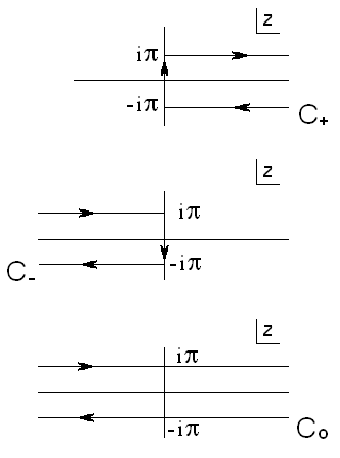
where in the last step the integral representation for the product of modified Bessel functions is used (see, e.g., [34]). Using the Schläfli contour integral representation
we perform summation over and get
| (23) |
where contours , and in the complex z-plane are shown in figure 2, and
| (24) |
Substituting the last line of (23) into (22), integrating over variables and , we get
Integrating over and changing variable to , we get final expression for the vacuum current
| (25) |
The vacuum current vanishes in the case of vanishing flux (), while in the case of vanishing tension () we get
| (26) |
and the result of [35] is recovered
| (27) |
Using the asymptotics of the Macdonald function at large values of the argument,
we get the asymptotics of the vacuum current at large distances from the brane:
| (28) |
4 Vacuum magnetic field
Assuming the valitity of the Maxwell equation
| (29) |
one can deduce that, owing to the induced angular component of the vacuum current, a magnetic field strength is also induced in the vacuum outside the brane, being directed along it:
| (30) |
note that coupling constant possesses dimension in -dimensional space-time. Substituting (25) into (30), we get expression
| (31) |
which decreases at large distances from the brane as
| (32) |
Consequently, the magnetic flux is induced in the vacuum outside the brane:
| (33) |
In the case of we get (see next section for details and compare with relation (41))
| (34) |
where is the Euler gamma function; this result can be analytically extended to a meromorphic function on the whole complex -plane, which in the physically meaningful domain has poles at real odd values of and is finite at real even values of .
However, it seems more reasonable to restrict the validity of (34) to the case of ,
| (35) |
while in the cases of cutoff at small distances to the brane should be introduced:
| (36) |
| (37) |
the integral in (37) can be explicitly taken in the case of real odd values of , see the next section.
5 Massless quantum matter
Using the asymptotics of the Macdonald function at small values of the argument, we get the vacuum current for the massless scalar field:
| (38) |
In the case of vanishing tension, the integral in (38) is taken, yielding [35]
| (39) |
In the case of nonvanishing tension, the integral in (38) is explicitly taken for odd values of only [28]. To see this, let us use the contour integral representation given by the first line in (23) and present (38) in another way
| (40) |
If is odd, then the integrand in (40) has a pole at and contour is deformed to encircle this pole, yielding
| (41) |
| (42) |
| (43) |
| (44) |
and so on; note that (41) was first obtained in [36]. If is even, then the integrand in (40) has a branch point singularity at .
Using (30), we get expression for the vacuum magnetic field strength:
| (45) |
Thus the induced vacuum flux is divergent either at small or at large distances from the brane, or both. In the case of , introducing cutoff at large distances from the brane, we get
| (46) |
In the cases of introducing cutoff at small distances to the brane, we get relation (37). In the case of the vacuum flux is logarithmically divergent both at small and at large distances from the brane, and, introducing both cutoffs, we get
| (47) |
6 Discussion
In the present paper we have obtained integral representation (25) for the induced vacuum current of the quantized charged massive scalar field in the cosmic string background. All the dependence on the cosmic string parameters (tension and flux ) is described by function (24), whereas the dependence on spatial dimension is factored otherwise. The Bohm-Aharonov effect is manifested in the periodic dependence of the vacuum current on flux with period , i.e. expression (25) depends on the fractional part of (18) rather than on quantity itself. Expression (25) vanishes at (i.e. at , where and ), being negative and convex downwards in the interval , while positive and convex upwards in the interval ; positions of the minimum and the maximum are symmetric with respect to the point . Expression (25) can be analytically extended to complex values of the space dimension yielding a holomorphic function of complex variable .
According to the Maxwell equation a magnetic field is generated by a direct current, and thus the magnetic field strength is also induced in the vacuum, being directed along the cosmic string, see (31). The dependence of the field strength on the cosmic string parameters and on the spatial dimension is qualitatively similar to that of the current. Both the current and the field strength decrease exponentially at large distances from the cosmic string, see (28) and (32). Both the current and the field strength increase as in the vicinity of the cosmic string, see (38) and (45). Thus the induced vacuum magnetic flux is finite in the case of only, see (35), whereas divergent otherwise, and a small vicinity of the cosmic string is eliminated by cutoff in the cases of , see (36) and (37); note that the flux is hence independent of mass in the cases of . In the case of , by identifying the cutoff with the transverse size of the core of the cosmic string, , we get
| (48) |
One can conclude that, if the mass of the quantized scalar is smaller than the mass of the Higgs scalar, , then the cosmic string is enclosed in a tube of the magnetic flux lines with the transverse size of the order of .
It should be noted that the vacuum current and, consequently, the vacuum magnetic field are odd under charge conjugation. The production of cosmic magnetic fields during cosmological phase transitions is currently discussed in the context of fundamental CP violation in particle physics, see [37]. As it follows from our consideration, topological defects (cosmic strings) appearing in the aftermath of phase transitions can produce magnetic fields via the vacuum polarization.
References
References
- [1] Vilenkin A and Shellard E P S 1994 Cosmic Strings and Other Topological Defects (Cambridge: Cambridge Univ. Press)
- [2] Hindmarsh M B and Kibble T W B 1995 Rep. Progr. Phys. 58 477
- [3] Misner C W, Thorne K S and Wheeler J A 1973 Gravitation (San Francisco: W H Freeman)
- [4] Nielsen H B and Olesen P 1973 Nucl. Phys. B 61 45
- [5] Weber J and Wheeler J A 1957 Rev. Mod. Phys. 29 509
- [6] Marder L 1958 Proc. Roy. Soc. London A 244 524
- [7] Marder L 1959 Proc. Roy. Soc. London A 252 45
- [8] Kibble T W B 1976 J. Phys. A: Math Gen. 9 1387
- [9] Kibble T W B 1980 Phys. Rep. 67 183
- [10] Vilenkin A 1981 Phys. Rev. D 23 852
- [11] Vilenkin A 1981 Phys. Rev. D 24 2082
- [12] Zeldovich Ya B 1980 Mon. Not. Roy. Astron. Soc. 192 663
- [13] Garfinkle D 1985 Phys. Rev. D 32 1323
- [14] Sarangi S and Tye S H H 2002 Phys. Lett. B 536 185
- [15] Jeannerot R, Rocher J and Sakellariadou 2003 Phys. Rev. D 68 103514
- [16] Polchinski J 2005 Int. J. Mod. Phys. A 20 3413
- [17] Brandenberger R H 2008 String gas cosmology Preprint arXiv: 0808.0746 [hep-th]
- [18] Vachaspati T 2009 Dark strings Preprint arXiv: 0902.1764 [hep-ph]
- [19] Sazhin M V, Khovanskaya O S, Capaccioli M, Longo L, Paolillo M, Covone G, Grogin N A and Schreier E J 2007 Mon. Not. Roy. Astron. Soc. 376 1731
- [20] Kaiser N and Stebbins A 1984 Nature 310 391
- [21] Battye R A, Garbrecht B, Moss A and Stoica H 2008 J. Cosmol. Astropart. Phys. JCAP0801 (2008) 020
- [22] Aharonov Y and Bohm D 1959 Phys. Rev. 115 485
- [23] de Sousa Gerbert P and Jackiw R 1989 Commun. Math. Phys. 124 229
- [24] Sitenko Yu A 1992 Nucl. Phys. B 372 622
- [25] Sitenko Yu A and Mishchenko A V 1995 JETP 81 831
- [26] Sitenko Yu A and Vlasii N D 2007 Proc. Gamov Memorial Int. Conf. ”Astrophysics and Cosmology after Gamov – Theory and Observations”, Odessa, Ukraine (Cambridge: Cambridge Univ. Press) p 299
- [27] Frolov V P and Serebriany E M 1987 Phys. Rev. D 35 3779
- [28] Dowker J S 1987 Phys. Rev. D 36 3095
- [29] Guimaraesh M E X and Linet B 1994 Commun. Math. Phys. 165 297
- [30] Guimaraesh M E X and Oliveira A L N 2003 Int. J. Mod. Phys. A 18 2093
- [31] Itzykson C and Zuber J-B 2006 Quantum Field Theory (New York: Dover)
- [32] Adami R and Teta A 1998 Lett. Math. Phys. 43 43
- [33] Dabrowski L and Stovicek P 1998 J. Math. Phys. 39 47
- [34] Prudnikov A P, Brychkov Yu A and Marychev O I 1986 Integrals and Series: Special Functions (New York: Gordon & Breach)
- [35]
Sitenko Yu A and Babansky A Yu 1998 Mod. Phys. Lett. A
13 379
Sitenko Yu A and Babansky A Yu 1998 Phys. Atom. Nucl. 61 1594 - [36] Sriramkumar L 2001 Class. Quantum Grav. 18 1015
- [37] Vachaspati T 2008 Magnetic fields in the aftermath of phase transition Preprint arXiv: 0802.1533 [astro-ph]