Fractal initial conditions and natural parameter values in hybrid inflation
Abstract
We show that the initial field values required to produce inflation in the two fields original hybrid model, and its supergravity F-term extension, do not suffer from any fine-tuning problem, even when the fields are restricted to be sub-planckian and for almost all potential parameter values. This is due to the existence of an initial slow-roll violating evolution which has been overlooked so far. Due to the attractor nature of the inflationary valley, these trajectories end up producing enough accelerated expansion of the universe. By numerically solving the full non-linear dynamics, we show that the set of such successful initial field values is connected, of dimension two and possesses a fractal boundary of infinite length exploring the whole field space. We then perform a Monte–Carlo–Markov–Chain analysis of the whole parameter space consisting of the initial field values, field velocities and potential parameters. We give the marginalised posterior probability distributions for each of these quantities such that the universe inflates long enough to solve the usual cosmological problems. Inflation in the original hybrid model and its supergravity version appears to be generic and more probable by starting outside of the inflationary valley. Finally, the implication of our findings in the context of the eternal inflationary scenario are discussed.
pacs
98.80.CqI Introduction
The paradigm of inflation [1, 2, 3, 4] is currently the simplest way to solve the standard cosmological problems and explain the Cosmic Microwave Background (CMB) anisotropies observed so far, though other alternative mechanisms have been proposed (for a review see [5] and references therein). Many models of inflation have been proposed [6, 7], based on single field or multi-field potentials. If single field models are efficient effective models, hybrid models explore the possibility that the inflaton is coupled to other scalar fields, as first proposed by Linde [8]. When coupled to a Higgs-type field, inflation is realized in the so-called “inflationary valley” when the Higgs vacuum expectation value (vev) vanishes and the inflation end is triggered when the Higgs becomes tachyonic and develops and non-vanishing vacuum expectation value (vev). Similar models have rapidly been constructed in various theoretical frameworks [9, 10, 11], the most popular of them being the supersymmetric/supergravity versions of F-term or D-term inflation [12, 13, 14, 15].
In the limit of sub-planckian field values, all hybrid inflation models were however thought to require extremely fine-tuned initial field values to produce enough e-folds of acceleration, from the original model proposed by Linde to most supersymmetric versions [16, 17, 18], with the exception of hilltop potentials which assume that inflation takes place near a maximum of the potential [19, 20]. The successful initial field values were found located only in an extremely narrow band around the inflationary valley, or on a few scattered points away from it [21]. This was considered as a fine-tuning problem for these models since any pre-inflationary era would have to be fine-tuned to allow inflation to last long enough to solve the standard cosmological problems. This fine-tuning has recently been revisited in Ref. [22] for the original hybrid model as well as for the supersymmetric “smooth” and “shifted” models. Using higher precision, it was shown that the successful initial field values are rather organised in intricate dense regions outside of the inflationary valley (see for instance Fig. 7 of Ref. [22]). The area occupied by these regions was found to represent up to of the sub-planckian field regime for the original hybrid model and up to for smooth hybrid inflation. The physical explanation of these new successful regions comes from the existence of an initial fast-roll phase during which the fields roll down the potential in a chaotic way followed by a climbing up of the valley and a slow-rolling phase back down.
However, as discussed in Ref. [22], these new successful regions appeared to depend on the shape of the potential, and therefore on the potential parameters. One may wonder whether these features are a new solution of the fine-tuning problem, i.e. if they are robust with respect to the potential parameters. Moreover, Ref. [22] did not discuss the statistical properties of this space and the effect of the initial field velocities which were assumed vanishing. Finally, the popular supersymmetric extensions, F- or D-term hybrid models, were not studied. The purpose of the present paper is to quantify how these new successful inflationary regions are widespread in the higher dimensional space of all the model parameters, i.e. by considering not only the initial field values but also their initial velocities and the potential parameters. We also extend our analysis to the F-term hybrid model, studied in SUGRA [12, 13].
In order to deal with a multi-dimensional parameter space, after having discussed the fractal nature of the successful inflationary regions, we introduce a probability measure and perform their exploration by using Monte–Carlo–Markov–Chains (MCMC) methods. The outcome of our approach is a posterior probability distribution on the model parameters, initial velocities and field values such that inflation lasts more than e-folds11 1 Such probability distributions are almost independent of the chosen number of e-folds: once the field rolls down in a flat enough region of the potential, the total number of e-folds generated is always very large.. As will be shown in the following, thanks to inflation starting “out of the valley”, a high number of e-folding appears to be generic, and favoured, in the original hybrid model for parameter ranges covering several orders of magnitude. We have also checked that such a result is not peculiar to a given potential by applying the same analysis to the more realistic two-field F-term inflation potential. This treatment allows us to establish natural bounds on the parameters (or combination of parameters) for each of these scenarios.
At this point, we would like to emphasize that our aim is not (yet) to constrain these models with the current Cosmic Microwave Background (CMB) and astrophysical data but rather to discuss in details their ability to generate an inflationary phase. In particular, in the small field limit, original hybrid model are known to generate a blue spectrum of scalar initial perturbations22 2 This conclusion can be altered when additional couplings are assumed for the inflaton [23]., which is disfavoured by recent CMB experiments [24]. Our use of this model here is motivated by its simplicity and its representativity of the non-linear two-field dynamics. The more realistic F-term SUGRA model is in agreement with the current CMB data: it predicts an almost scale invariant spectrum and the generic formation of cosmic strings [25], a combination which was shown to be favoured by observations in Ref. [26].
The paper is organised as follows. In the following section, we discuss the fractal nature of the successful regions of inflation in the original hybrid model and define a probability measure over the full parameter space. In Sec. III, the MCMC method is introduced and we study step by step the effect of the initial field velocities and the potential parameters on the probability of obtaining e-folds of inflation. We then present the full posterior probability distributions of these parameters for the original hybrid scenario. In Sec. IV, we perform the same analysis of the F-SUGRA hybrid potential. Some conclusions and perspectives are finally presented in the last section.
II Fractal initial field values
II.1 The model
The original hybrid model of inflation was proposed in Refs. [8, 13], its potential reads
| (1) |
The field is the inflaton and is the auxiliary Higgs-type field while , are two positive coupling constants and , are the two mass parameters. Inflation is assumed to be realized in the false-vacuum along the valley33 3 Throughout the paper denotes the vev of a field. and ends due to a tachyonic instability of when the inflaton reaches a critical value . The classical system evolves toward its true minimum , and whereas in a realistic scenario one expects the tachyonic instability to trigger a preheating era [27, 28, 29, 30, 31, 32].
To observe the effects of varying the free parameters in the dynamics of inflation, it is more convenient to rewrite the potential into
| (2) |
under which are three mass parameters. With this expression, the critical point of instability now reads
| (3) |
It is common usage to consider the effective one-field potential by restricting the field dynamics to the inflationary valley and one gets
| (4) |
II.2 Equations of motion
In a flat Friedmann--Lemaître-Robertson--Walker (FLRW) metric, the equations governing the two-field dynamics are the Friedmann-Lemaître equations44 4 Throughout the paper, denotes the physical Planck mass, and stands for the reduced Planck mass GeV.,
| (5) |
as well as the Klein-Gordon equations
| (6) |
where is the Hubble parameter, is the scale factor and a dot denotes derivative with respect to cosmic time.
In order to study the two-fields dynamics of the hybrid model, without assuming slow-roll, one has to integrate these equations numerically from a given set of initial conditions (IC) for the field values. Throughout the paper we will define a successful IC as a point in field space that lead to a sufficiently long phase of inflation to solve the horizon and flatness problem. We will assume that e-folds is the critical value required, though this value can change by a factor of two depending on the reheating temperature and the Hubble parameter at the end of inflation [33, 34]. However, generically, once inflation starts it lasts for much more than e-folds and our results are not sensitive to the peculiar value chosen.
II.3 The set of successful initial field values

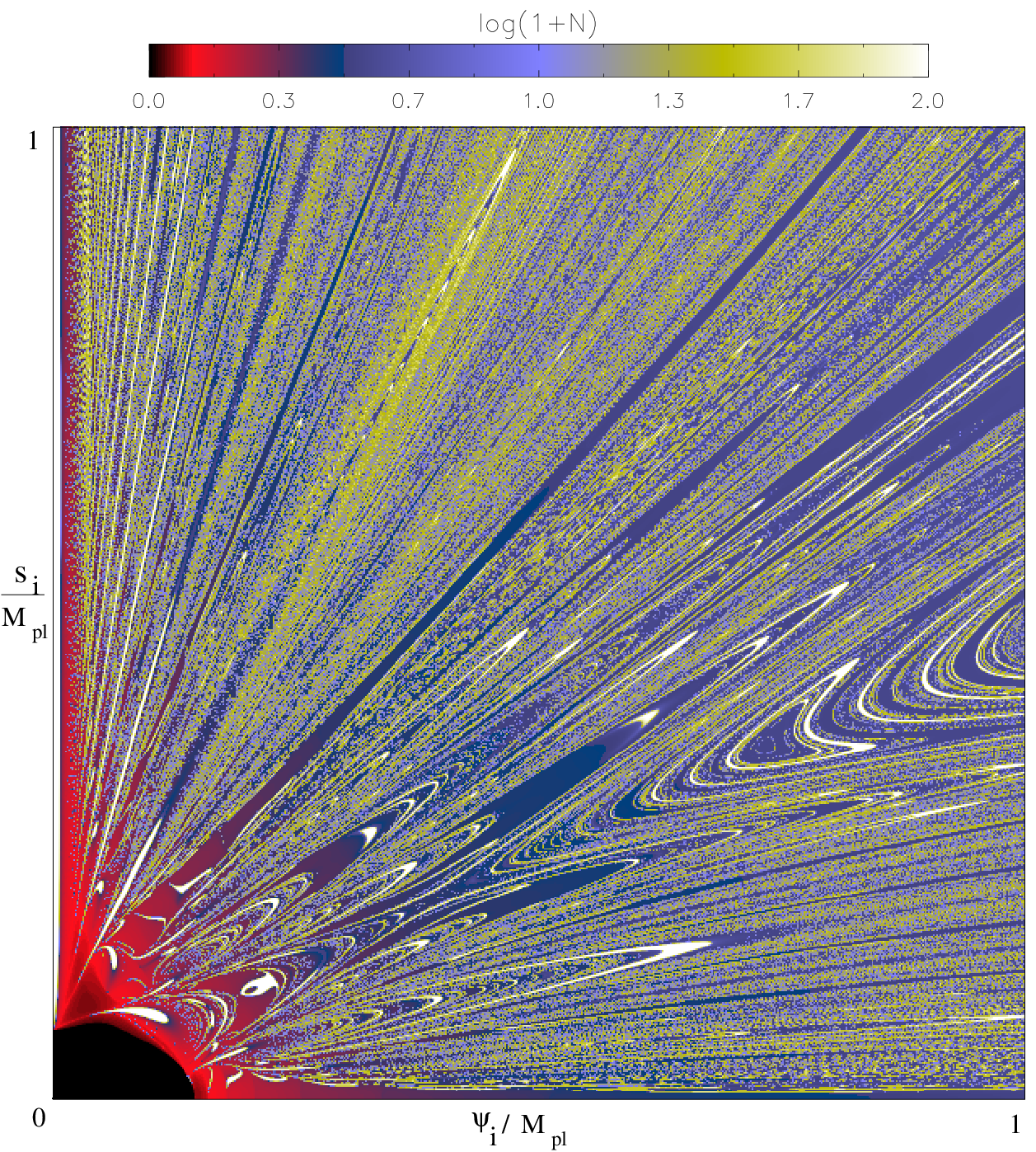
As already mentioned in the introduction, the space of successful IC for the field values alone has been discussed in Ref. [22] and found to be composed of a intricate ensemble of points organized into continuous patterns. In Fig. 1, we have represented the mean number of e-folds generated at each sub-Planckian initial field values, for a set of fixed potential parameters and assuming vanishing initial velocities. We have computed the trajectories obtained from initial field values and stopped the integration when the fields are trapped in one of the minimum of the potential, i.e. for , or when the accelerated expansion exceeds efolds. The resulting grid has a small intricated structure of successful regions spread over the whole plane which ends up being difficult to represent in a figure. As a result, we have chosen to present in Fig. 1 a downgraded pixels image in which each pixel has been given a color according to the average number of e-folds obtained in our original grid. A given pixel may therefore hide both successful and unsuccessful initial field values and the color measures their relative density. An higher resolution image would be self-similar to Fig. 1, with more thinner successful domains visible.
Notice that we recover the inflationary valley as the white vertical narrow strip located along whereas the minima of the potential are along the horizontal axis at (for as chosen in the figure). The black region in Fig. 1 precisely corresponds to the trajectories “below” the critical point which are fast-rolling inside the minima. In analogy with the anamorphosis of light produced by a distorted mirror, each point outside the inflationary valley is connected by a trajectory to a point inside the inflationary valley. The trajectory first fast-rolls towards the bottom of the potential, and after a few rebounds becomes oriented along the valley, climbs it and then produces inflation when slow-rolling back down. There is thus a one-to-one correspondence between the IC and the point in the valley for which the trajectory stops to climb and starts to slow-roll.
It was shown in Ref. [22] that such “anamorphosis points” can cover up to of the total area when restricting the IC to sub-planckian values. Moreover, as can be checked in Fig. 1, these regions exhibits a fractal looking aspect. Before studying the influence of the potential parameters and initial field velocities, one may wonder if the area of this two-dimensional set of points is indeed well-defined? Equivalently, do new successful regions appear inside unsuccessful domains and conversely? In order to quantify how much the anamorphosis points are a probable way to have inflation in the whole parameter space, we first address the question of defining a measure on the initial field values space. In particular, this requires to determine the dimension of the set
| (7) |
II.4 Chaotic dynamical system
II.4.1 Phase space analysis
As suggested by Fig. 1, at fixed potential parameter values, the dynamical system defined by Eqs. (5) and (6) seems to exhibit a chaotic behaviour. In particular, the sensitivity of the trajectories to the initial field values comes from the presence of three attractors. Two of them are the global minima of the potential, respectively at , in which all classical trajectories will end, whereas the less obvious is a quasi-attractor defined by the inflationary valley itself (, ). Indeed, whatever the initial field values, as soon as the system enters slow-roll one has (in Planck units) [35],
| (8) |
where is the first Hubble flow function [36]. The system therefore spends an exponentially long amount of cosmic time in the valley. The sensitivity to the initial conditions comes from the presence of these three attractors: either the trajectory ends rapidly into one of the two minima, or it lands on the valley where it freezes.

A phase space plot is represented in Fig. 2 in which we have computed trajectories from a grid of initial field values. The inflationary valley clearly appears as the attractor with quasi null velocity vector (), while around the two global minima, two “towers” appear due to the field oscillations around them.
II.4.2 Basins of attraction
From the definition of in Eq. (7), one has
| (9) |
where stands for the mapping induced by the differential system of equations (5) and (6). The set of successful initial field values is therefore the basin of attraction of the attractor [37, 38]. Since the attractor is a dense set of dimension 2 and is continuous, one expects to contain a dense set of dimension 2 [38]. As can be intuitively guessed, the boundary of can however be of intricate structure because of the sensitivity to the initial conditions: two trajectories infinitely close initially can evolve completely differently. As we show in the following, is actually a set of dimension two having a fractal boundary of dimension greater than one.
Finally, by the definition of a continuous mapping, all parts of , boundary included, must be connected together and to the inflationary valley . The fractal looking aspect of Fig. 1 is only induced by the intricate boundary structure of which is exploring all the initial field values space. The fractality of the boundaries of the space of initial fields values was first mentioned in Ref. [39], but the study was restricted to a small region of the field space and the model included dissipative coefficients. As an aside remark, let us notice that the existence of a fractal boundary may have strong implications in the context of eternal chaotic inflation: there would exist inflationary solution close to any initial field values.
In order to quantify the chaotic properties of the dynamical system defined by the mapping , we turn to the calculation of the Lyapunov exponents.
II.4.3 Lyapunov exponents

The Lyapunov exponents at an initial point measures how fast two infinitely close trajectories mutually diverge or converge. They give a mean to characterize the stretching and contracting characteristics of sets under the mapping induced by the differential system. A small perturbation around the trajectory will evolve according to
| (10) |
where stands for the Jacobian of the differential system . The Lyapunov exponents at the initial point and along the direction are the numbers defined by [37]
| (11) |
where is the solution of Eq. (10) with and . If the considered set is an attractor or an invariant set of the differential system having a natural measure, one can show that the exponents do not depend on the initial point . At fixed potential parameters, there are four Lyapunov exponents associated with the differential system of Eqs. (5) and (6). If the largest exponent is positive, then the invariant set is chaotic.
In Fig. 3, we have computed the largest Lyapunov exponent at each point of the plane . The numerical method we used is based on Refs. [40, 41] and uses the public code LESNLS. Let us notice that since is only a quasi-attractor, we have stopped the evolution at most when , i.e. just before the fields would classically enter either or . As can be seen, all points belonging to exhibit the same and small negative Lyapunov exponent: the invariant set is therefore non-chaotic. On the other hand, all the other initial field values associated with the basins of attraction of have a positive Lyapunov exponent. For those, the field evolution is chaotic and exhibits a sensitivity to the initial conditions. Notice that these exponents may slightly vary from point to point due to our choice to stop the integration at instead of the classical attractors . This is particularly visible for the trajectories starting close to (green shading): there is not enough evolution to get ride of the transient evolution associated with the initial conditions.
II.5 Fractal dimensions of and its boundary
II.5.1 Hausdorff and box-counting dimension
Since we suspect a set with fractal properties, the natural measure over , extending the usual Lebesgue measure, is the Hausdorff measure. The -dimensional Hausdorff measure of is defined by [38]
| (12) |
In this definition, the sets form a -covering of and the diameter function has been defined by . As a result, is the smallest sum of the th powers of all the possible diameters of all sets covering , when . Having such a measure, the fractal dimension of is defined to be the minimal value of such that the Hausdorff measure remains null (or equivalently the maximal value of such that the measure is infinite). In practice, measuring the Hausdorff dimension using this definition is not trivial, due to the necessity of exploring all -coverings. However, in our case, we are interested in the fractal properties of a basin of attraction associated with a continuous dynamical system and one can instead consider the so-called box-counting dimension [38]. This method simply restricts the class of the to a peculiar one, all having the same diameter . When the mapping is self-similar, one can show that box-counting and Hausdorff dimensions are equal. In general, the Hausdorff dimension is less or equal than the box-counting one. Here, being a contracting continuous flow, we expect the equality to also hold.
To define the box-counting dimension, we cover the set with grids of step size , and count the minimal number of boxes necessary for the covering. The box-counting dimension is then given by
| (13) |
This method has the advantage to be easily implemented numerically and, in the following, we will apply it to calculate the dimension of and its boundary.
II.5.2 Fractal boundary of
For each randomly chosen point of the plane , we compute three trajectories. The first one starts from the point under consideration while the two others have initial conditions modified by and along one direction (for example along , but the chosen direction does not affect the result). For each of these trajectories, we determine in which attractor ( or ) the flow ends. Since we are interested in the boundary of , we calculate the proportion of points for which at least one trajectory ends in , and another in or . The process is iterated for increasingly smaller values of and we evaluate how the area of the -grid covering of scales with . So strictly speaking, our evaluation of the box-counting dimension is made through the determination of the Minkowski dimension of the boundary of [38]. From Eq. (13), assuming that, at small ,
| (14) |
the box-counting dimension of the boundary is then given by [37]
| (15) |

In Fig. 4, we have plotted as a function of at fixed potential parameters. We recover the expected power law behaviour, the slope of which is approximately . As a result, the boundary of is indeed a fractal of box-counting dimension
| (16) |
Notice that this value depends on the chosen set of potential parameters, as one may expect since they affect the shape of and the typical size of the structures.
II.5.3 Dimension of
In order to determine the box-counting dimension of itself one can apply a similar method than the one used for its boundary. Now denotes the proportion of points for which at least one of the three trajectories end in the attractor (this condition therefore includes also the points belonging to the boundaries). The resulting power-law is represented in Fig. 5.

For small enough values of , the -sized boxes are small enough to be fully contained in and the function appears to be constant in that case. As a result, the box-counting dimension of is . We therefore conclude that, like for the well-known Mandelbrot set [42], the boundary of is fractal but the set of successful inflationary points is not and has the dimension of a surface. Consequently, although the boundary of has an infinite length (), it has a vanishing area: the Hausdorff dimension of (boundary included) is therefore also 2. As a result, the two-dimensional Hausdorff measure on reduces to the usual two-dimensional Lebesgue measure and this will be our choice for defining a probability measure in the rest of the paper.
As previously emphasized, the potential parameters and initial field velocities have been fixed in this section and the set is actually the two-dimensional section of an higher dimensional set, whose boundary is also certainly fractal (and therefore of null measure). Since one can no longer use griding method to explore such a high dimensional space, we move on in the next section to a MCMC exploration of the full parameter space to assess the overall probability of getting inflation in the hybrid model.
III Probability distributions in hybrid inflation
The aim of this section is to use Monte-Carlo-Markov-Chains (MCMC) techniques in order to explore the whole parameter space, including the initial field velocities and all the potential parameters. With unlimited computing resources, we could have used a griding method to localise the hypervolumes in which inflation occurs, as we have done for the two-dimensional plane in the previous section. For the original hybrid model, we have in total seven parameters that determine a unique trajectory: two initial field values, initial field velocities and the three potential parameters , and . To probe this seven-dimensional space, more than just measuring the hypervolume of the successful inflationary regions, we define a probability measure over the full parameter space. Using Bayesian inference, one can assess the posterior probability distribution of all the parameters to get enough e-folds of inflation. Monte–Carlo–Markov–Chains (MCMC) method is a widespread technique to estimate these probabilities, its main power being that it numerically scales linearly with the number of dimensions, instead of exponentially.
Several algorithms exist in order to construct the points of a Markov chain, the Metropolis–Hastings algorithm being probably the simplest [43, 44]. Each point , obtained from a Gaussian random distribution (the so-called proposal density) around the previous point , is accepted to be the next element of the chain with the probability
| (17) |
where is the function that has to be sampled via the Markov chain. MCMC methods have been intensively used in the context of CMB data analysis [45, 46, 47, 48, 49] where the function is the posterior probability distribution of the model parameters given the data. In the context of Bayesian inference, this one is evaluated from the prior distributions and the likelihood of the experiment . After a relaxation period, one can show that Eq. (17) ensures that is the asymptotic stationary distribution of the chain [50]. The MCMC elements directly sample the posterior probability distribution of the model given the data.
In our case, we can similarly define a likelihood as a binary function of the potential parameters, initial field values and velocities. Either the trajectory ends up on and produces more than e-folds of inflation, or it does not. In the former case we set whereas for no inflation. The function we sample is then defined by where stands for field values, velocities and potential parameters and is our prior probability distribution that we will discuss in the next section.
III.1 Prior choices
MCMC methods require a prior assumption on the probability distributions of the fields, velocities and potential parameters. As we only consider in this work the initial conditions and parameters space leading to at least e-folds of inflation, the prior choices are only based on theoretical arguments. These arguments can be linked to the framework from which the potential is deducted. If one considers the hybrid model to be embedded in supergravity, the fields have to be restricted to values less than the reduced Planck mass. We adopt here this restriction for initial field values, not only because of this argument, but also because it has been shown in Ref. [22] that if super-plankian fields are allowed, trajectories become generically successful. On the other hand, the model was considered to suffer some fine-tuning when one of the fields has to be order of magnitudes smaller than the other. As inflation is not possible for very small initial values of both fields (because of the Higgs instability), we have considered a flat prior for initial field values in as opposed to a flat prior for the logarithm of the fields. Note that one has to include negative values of the fields in order to take into account the orientation of the initial velocity vector.
Concerning the initial field velocities, from the equations of motion, one can easily show that there exist a natural limit55 5 This is just the limit in Planck units [35].
| (18) |
Similarly, our prior choices are flat distributions inside such a circle in the plane , where “” denotes a partial derivative with respect to the number of e-folds.
In the absence of a precise theoretical setup determining the potential there are no a priori theoretical constraint on its parameters , and . Let us just mention that for , the dynamics of inflation in the valley is possibly strongly affected by slow-roll violations [22]. As a result, with the concern to not support a particular mass scale, we have chosen the following flat priors on the logarithm of the parameters:
| (19) | ||||
in which the upper and lower limits have been set for numerical convenience, and .
Notice that the dependencies are not important here because this parameter only rescales the potential and thus does not change the dynamics.
In the next sections, we perform the MCMC exploration of the parameter space from these priors. Firstly by reproducing the results of Sec. II in the two-dimensional section , then by including the initial field velocities and finally by considering all the model parameters. Unless otherwise mentioned, the chains contain points, which corresponds to one percent error on the marginalised probability distributions. In the figures, the overall values of the posterior probability density distributions have not been represented since they are determined by the imposing the integral over the parameters to be equal to one.
III.2 MCMC on initial field values

In order to test our MCMC, we have first explored the space of initial field values leading or not to more than e-folds of inflation. The potential parameters have been fixed to various values already explored by griding methods in Sec. II and Ref. [22], while the initial velocities are still assumed to vanish. The MCMC chain samples have been plotted in Fig. 6. Notice that to recover the fractal structure of the boundary of , one has to adjust the choice of the Gaussian widths of the proposal density distribution. If those are too large, the acceptance rate will be small because the algorithm tends to test points far away from the last successful point, and if they are too small the chains remain stuck in the fractal structures without exploring the entire space. Nevertheless, with an intermediate choice, Fig. 6 shows that the intricate structure of the boundary of can be probed with the MCMC. More than being just an efficient exploration method compared to griding, the MCMC also provides the marginalised probability distributions of and such that one gets inflation. They have been plotted in Fig. 10 (top two plots), the normalisation being such that their integral is unity. As one can guess from Fig. 6, with vanishing initial velocities and a fixed set of potential parameters, inflation starting in the valley is not the preferred case since the area under the distribution of outside of the valley is larger than inside. Moreover, these distributions take non-vanishing values everywhere and there is therefore no fine-tuning problem. Of course, one still have to consider the other parameters and this is the topic of the next sections.
III.3 MCMC on initial field values and velocities

The initial values of the field velocity are inside a disk of radius in the plane (in Planck units). The marginalised two-dimensional posteriors for the initial field values is plotted in Fig. 7 whereas the marginalised posterior for each field are represented in Fig. 10 (middle line). Even if non-vanishing velocities are considered, the successful inflationary patterns remain. Notice that they appear to be blurred simply because of the weighting induced by marginalising the full probability distribution over the initial velocities.

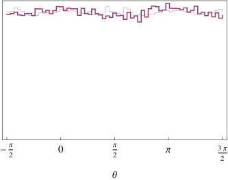
In Fig. 8, we have also represented the marginalised posterior probability distribution for the modulus and direction of the initial velocity vector. Their flatness implies that there are no preferred values. This is an important result because one could think that large initial velocities could provide a way to kick trajectories in or out of the successful regions. This actually never happens because of the Hubble damping term in the Friedmann equations, allowing only a generation of a small number of e-folds before the trajectory falls in one of the three attractors.
III.4 MCMC on initial field values, velocities and potential parameters


The most interesting part of the exploration by MCMC technique concerns the study of the full parameter space. The only restriction being associated to the necessity of as discussed in Sec. III.1. The chains contain elements and the estimated error on the posteriors is about a few percents.
We have plotted in Fig. 9 the marginalised two-dimensional posterior for the initial field values. In comparison with Fig. 6 and 7, the most probable initial field values are now widespread all over the accessible values; the intricate patterns that were associated with the successful field values (at fixed potential parameters) are now diluted over the full parameter space. The resulting one-dimensional probability distributions for each field are plotted in Fig. 10 (bottom panels). One can observe that the distribution is nearly flat outside the valley but remains peaked around a extremely small region around . Integrating over the field values, initial conditions outside the valley are still the preferred case.
Concerning the probability distributions of the modulus and the angular direction of the initial velocity vector, results integrated over the whole parameter space do not present qualitative differences compared to the posteriors with fixed potential parameters, as one may expect since the Hubble damping prevents the initial velocities to influence the dynamics (see Fig. 8).


The marginalised probability distributions for the potential parameters are represented in Fig. 11. These posteriors seem to indicate that the three parameters are bounded but one should pay attention to the influence of our prior choices over the posterior [51]. In fact, the posteriors for and are found to depend on our prior choice: changing the upper or lower limit on the -prior (or -prior) affects the values at which the - and -posteriors fall off. Such a situation is typical of the existence of correlations between these two parameters. We have therefore computed the two-dimensional posterior distribution in the plane and found out that this probability distribution clearly exhibits a correlation between these two parameters: the lower bound on depends on the minimal allowed value of in the prior. Such a correlation comes from the fact that, to realize enough inflation for a given IC, the critical/instability point should not be larger than the anamorphosis image of the IC (the point in the valley where slow-roll starts). Restricting initial fields to sub-Planckian values leads to an uper bound on the largest image, and thus an upper bound on the instability point. From Eq. (3), the relevant quantity that is constrained is the combination .

We have plotted in Fig. 12 the marginal posterior distribution associated with the parameter , and at of confidence level, we find
| (20) |
The parameter is the other constraint that the MCMC exibits. It is explained by the possible apparition of slow-roll violations in the valley, when becomes too small. These slow-roll violations prevent the generation of an inflationary phase if the trajectory climbs too high in the valley. At a two-sigma level, one has
| (21) |
This lower limit is equivalent to the upper limit on observed in [22]: a large inflaton mass induces a fast roll evolution and requires super-planckian initial conditions to realize inflation in a chaotic way. Let us stress that these constraints come only from requiring enough inflation in the hybrid model whatever the initial field values, velocities, and other potential parameters. In this respect, the limits of Eqs. (20) and (21) can be considered as “natural”.
To conclude this section, we have shown that inflation is generic in the context of the hybrid model and we have derived the marginalised posterior probability distributions of all the parameters such that 60 e-folds of inflation occur. As discussed in the introduction, the original hybrid model under scrutiny is however a toy model known to be disfavored by the current CMB data. In this respect, one may wonder whether our results are peculiar to this model or can be generalised to other more realistic two field inflationary models. This point is addressed in the next section in which we have performed a complete study of the SUGRA F-term hybrid inflation. In that model, the dynamics depends on only one potential parameter; also constrained by cosmic strings formation. The challenge will thus be to confront this constraint to the natural bounds that can be deducted from MCMC methods by requiring enough e-folds of inflation.
IV Probability distributions in F-SUGRA inflation
The minimal supersymmetric versions of hybrid inflation are known as the F-term and D-term inflationary models [12, 14, 15], where the slope of the valley is generated by radiative corrections. The F-term model is compatible with the current CMB data since a red spectrum of the cosmological perturbations is generic [12, 52, 53]. In addition, this model is more predictive and testable than its non-SUSY version since it contains only one coupling constant and one mass scale.
IV.1 The model
In the following, we are analysing the space of initial conditions and model parameters leading to enough inflation for the so-called F-term model based on the superpotential [12]
| (22) |
The inflaton is contained in the superfield . The Higgs pair is charged under a gauge group , that is broken at the end of inflation when the Higgs pair develop a non-vanishing expectation value (vev) . The superpotential leads in global SUSY to a tree level potential
| (23) |
where the effective inflaton and Higgs field can be made real and canonically normalized [, ]. The local minima of the potential at large provide a flat direction for the inflaton : .
This tree level flat direction is lifted by two effects. Firstly, radiative corrections are induced by the SUSY breaking that supports inflation. In addition, if the field values are close to the reduced Planck mass , one should expect supergravity corrections to the tree level potential. The radiative corrections along the inflationary valley can be derived using the Coleman-Weinberg formula [54]. They reduce to [12]
| (24) |
where , stands for the dimensionality of the representations to which belong and represents a non-physical energy scale of renormalization. Realistic values of can be derived from the embedding of the model in realistic SUSY Grand Unified Theories (GUT) as shown in Ref. [25]. For example, in the case of an embedding of the model in SUSY SO(10), belong to the representation or . However, as pointed out in Ref. [55], it is possible that only some components of take a mass correction of order so that effectively66 6 This depends on the mass spectrum of the assumed GUT model. . For the sake of generality, we will assume that can take values in the range . This model is also known to generically produce cosmic strings at the end of inflation [25] and this imposes an upper limit on the inflationary mass scale [56, 53, 55]
| (25) |
Secondly, SUGRA corrections also contribute to lifting the tree-level flat direction and will be taken into account since the field values we are probing are not always negligible compared to the Planck mass. It has been noticed in Ref. [13] that the F-term hybrid inflation model doesn’t suffer from the -problem only when the Kähler potential is (close to) minimal77 7 We will restrict ourselves to minimal SUGRA corrections, neglecting SUSY breaking soft terms and the non-renormalizable corrections to the superpotential (see [52, 53, 55] for an analysis of their effects).
| (26) |
which is what we assume in the following. In terms of the canonically normalized effective inflaton and waterfall fields , the SUGRA corrected potential now reads
| (27) |
The dynamics along the inflationary valley is driven by the radiative corrections and by the SUGRA corrections. The radiative corrections play a major role in the last e-folds of inflation (thereby generating the observable spectral index), whereas most of the dynamics takes actually place for field values dominated by the SUGRA corrections. We have calculated the amplitudes for both corrections and found that only at the end of the inflationary potential (for if and if ), the radiative corrections may dominate over the SUGRA corrections. In the present work, the regions of the parameter space leading to inflation do not depend on the very last part of the field evolution: as soon as e-folds are obtained, the initial conditions are considered successful and this generically occurs in the valley at larger field values. Outside the inflationary valley, we therefore expect the tree level dynamics to dominate over the radiative corrections, especially for small coupling . There also, in addition to the tree level, at large fields, SUGRA corrections are expected to be important.
Resulting of these considerations, we have neglected radiative corrections and used for our study below the potential of Eq. (27).
IV.2 Fractal initial field values
The analysis of the SUGRA F-term model of inflation has been conducted along the lines described in Sec. II and Sec. III. We have first verified that, at fixed potential parameter and vanishing initial velocities, the set of initial field values defined by Eq. (7) is two-dimensional with a fractal boundary. In Fig. 13, we have represented the set of successful initial field values for the mass scale . Notice that the coupling constant being an overall factor, it doesn’t impact the dynamics of the fields. Our study is therefore valid for any value of and of the dimensionality of the Higgs field , since the relationship depends only on .
As for the original hybrid model, the highest Lyapunov exponent for the successful initial field values is negative and the set is non-chaotic. Outside of , trajectories have positive Lyapunov exponents and exhibit chaos.
| Values of | Area of (%) |
|---|---|
| 0 (exact) | |
For vanishing initial velocities, we have reported in Table 1 the area occupied by the set in the plane for various section along the potential parameter . Like for the original hybrid model, we recover a significant proportion of successful initial field values outside the valley. This result holds even for though at small M, the potential becomes very flat and the number of oscillations of the system before being trapped in the inflationary valley can exceed . Simulations become therefore more time-consuming and error-bars in Tab. 1 increase. Reducing also reduces the typical size of structures in the plane , which evolves from Fig. 13 to a more intricated space of thinner successfull IC. As suggested by the Tab. 1, we will see below that this doesn’t affect the probability of getting inflation by starting the field evolution outside the valley.

Concerning the fractal properties of , we have applied the same method as in Sec. II.5.1 to compute the box-counting dimensions of and its boundary. As expected, we recover that is of box-counting dimension two whereas the function for its boundary is represented in Fig. 14. We obtain that, as in the non-SUSY case, the boundaries are fractal with dimension
| (28) |
These results allow us to use the usual Lebesgue measure to define the probability distribution over the whole parameter space.
IV.3 MCMC on the initial field values, velocities and the potential parameter

As already mentioned, there is only one potential parameter in F-term SUGRA model that may influence the two field dynamics. The goal of this section is to evaluate the probability distributions of the initial field values, velocities and of such that inflation lasts more than e-folds. As for the original hybrid model, we have performed an MCMC analysis on the five-dimensional parameter space defined by , , , and where
| (29) |
We have chosen the same sub-planckian priors for the initial field values and initial velocities than in Sec. III. Since the order of magnitude of is not known, we have chosen a flat prior on
| (30) |
The lower limit on is motivated by computational rather than physical considerations. The resulting marginalised posterior probability distributions for each of the parameters are represented in Fig. 15. The chains contain samples producing an estimated error on the posteriors around a few percent (from the variance of the mean values between different chains).

The posteriors for the field velocities are flat showing that all values are equiprobable to produce inflation. The initial field values are also flat, up to a sharp peak of higher probability density around corresponding to the inflationary valley. As for the hybrid model of Sec. II, after integration of these curves over the field values, inflation is clearly more probable by starting out of the valley. Finally, only the posterior probability distribution of is strongly suppressed at large values. We find, at of confidence level (see Fig. 16).
| (31) |
As for the original hybrid model, this limit comes from the condition of existence of a sub-planckian inflationary valley which is related to the position of the instability point. Indeed, from Eq. (27), one finds
| (32) |
where we have kept only the sub-planckian solutions. This expression shows that there is an inflationary valley at only for , and for field values such that . As a result of the two-field dynamics, we find that a valley supporting at least e-folds of inflation require the more stringent bound of Eq. (31). Let us finally notice that the most probable values we obtain on to get inflation in Eq. (31) are compatible with the existing upper bound coming from cosmic strings constraint: (see Ref. [56, 53]).
V Conclusion
In this paper, by numerically solving the two-field dynamics of the original hybrid model and its SUGRA F-term version, we have shown that e-folds of inflation is a generic outcome. Contrary to what is usually assumed, one does not need to fine-tune the initial field values around to get inflation. In fact, the inflationary valley, indeed of small extension in field space, is one of the three dynamical attractors of the differential system given by the Einstein and Klein–Gordon equations in a FLRW universe (the others being the minima of the potential). As a result, any trajectory will end in one of these three attractors and the set of successful initial conditions therefore belongs to the basin of attraction of the inflationary valley. We have shown that such a set is connected and of dimension two while exhibiting a fractal boundary of dimension greater than one. Moreover, it occupies a significant fraction of the sub-planckian field regime. In order to quantify what are the natural field and parameter values to get inflation for both of these models, we have introduced a probability measure and performed a MCMC exploration of the full parameter space. It appears that the inflationary outcome is independent of the initial field velocities, is more probable when starting out of the inflationary valley, and favours some “natural” ranges for the potential parameter values that cover many order of magnitudes. The only constraints being that the inflationary valley should at least exist.
Let us notice that the posterior probability distributions we have derived are not sensitive on the fractal property of the boundary of . This is expected since, even fractal, the boundary remains of null measure compared to . However, its existence may have implications in the context of chaotic eternal inflation [57, 58]. Indeed, the boundary itself leads to inflation and spawn the whole field space such that its mere existence implies that inflationary bubbles starting from almost all sub-planckian field values should be produced. Here, we have been focused to the classical evolution only and our prior probability distributions have been motivated by theoretical prejudice (flat sub-planckian prior). In the context of chaotic eternal inflation, our results are however still applicable provided one uses the adequate prior probabilities which are the outcome of the super-Hubble chaotic structure of the universe [59]. Provided the eternal scenario does not correlate with the classical dynamics, one should simply factorise the new priors with the posteriors presented here to obtain the relevant posterior probability distributions in this context.
Acknowledgements.
It is a pleasure to thank T. Carletti, S. Colombi, G. Esposito-Farese, A. Fuzfa, A. Lemaitre, J. Martin, P. Peter, and M. Tytgat for discussions and comments. S.C. is supported by the Belgian Fund for research (F.R.I.A.). J.R. is funded in part by IISN and Belgian Science Policy IAP VI/11.References
- [1] A. A. Starobinsky, Phys. Lett. B91, 99 (1980).
- [2] A. H. Guth, Phys. Rev. D23, 347 (1981).
- [3] A. D. Linde, Phys. Lett. B108, 389 (1982).
- [4] M. Lemoine, J. Martin, and P. Peter (Eds.), Inflationary cosmology, Lect. Notes Phys. 738 (Springer, Heidelberg, 2008).
- [5] P. Peter and N. Pinto-Neto, Phys. Rev. D78, 063506 (2008), eprint 0809.2022.
- [6] D. H. Lyth and A. Riotto, Phys. Rept. 314, 1 (1999), eprint hep-ph/9807278.
- [7] A. D. Linde (2005), eprint hep-th/0503203.
- [8] A. D. Linde, Phys. Rev. D49, 748 (1994), eprint astro-ph/9307002.
- [9] G. Lazarides and C. Panagiotakopoulos, Phys. Rev. D52, R559 (1995), eprint hep-ph/9506325.
- [10] R. Jeannerot, S. Khalil, G. Lazarides, and Q. Shafi, JHEP 10, 012 (2000), eprint hep-ph/0002151.
- [11] R. Kallosh and A. Linde, JCAP 0310, 008 (2003), eprint hep-th/0306058.
- [12] G. R. Dvali, Q. Shafi, and R. K. Schaefer, Phys. Rev. Lett. 73, 1886 (1994), eprint hep-ph/9406319.
- [13] E. J. Copeland, A. R. Liddle, D. H. Lyth, E. D. Stewart, and D. Wands, Phys. Rev. D49, 6410 (1994), eprint astro-ph/9401011.
- [14] P. Binétruy and G. R. Dvali, Phys. Lett. B388, 241 (1996), eprint hep-ph/9606342.
- [15] E. Halyo, Phys. Lett. B387, 43 (1996), eprint hep-ph/9606423.
- [16] G. Lazarides, C. Panagiotakopoulos, and N. D. Vlachos, Phys. Rev. D54, 1369 (1996), eprint hep-ph/9606297.
- [17] N. Tetradis, Phys. Rev. D57, 5997 (1998), eprint astro-ph/9707214.
- [18] G. Lazarides and N. D. Vlachos, Phys. Rev. D56, 4562 (1997), eprint hep-ph/9707296.
- [19] L. Boubekeur and D. H. Lyth, JCAP 0507, 010 (2005), eprint hep-ph/0502047.
- [20] K. Kohri, C.-M. Lin, and D. H. Lyth, JCAP 0712, 004 (2007), eprint 0707.3826.
- [21] L. E. Mendes and A. R. Liddle, Phys. Rev. D62, 103511 (2000), eprint astro-ph/0006020.
- [22] S. Clesse and J. Rocher, Phys. Rev. D79, 103507 (2009), eprint 0809.4355.
- [23] M. U. Rehman, Q. Shafi, and J. R. Wickman (2009), eprint 0901.4345.
- [24] E. Komatsu et al. (WMAP), Astrophys. J. Suppl. 180, 330 (2009), eprint 0803.0547.
- [25] R. Jeannerot, J. Rocher, and M. Sakellariadou, Phys. Rev. D68, 103514 (2003), eprint hep-ph/0308134.
- [26] N. Bevis, M. Hindmarsh, M. Kunz, and J. Urrestilla, Phys. Rev. Lett. 100, 021301 (2008), eprint astro-ph/0702223.
- [27] L. Kofman, A. D. Linde, and A. A. Starobinsky, Phys. Rev. D56, 3258 (1997), eprint hep-ph/9704452.
- [28] J. Garcia-Bellido and A. D. Linde, Phys. Rev. D57, 6075 (1998), eprint hep-ph/9711360.
- [29] G. N. Felder et al., Phys. Rev. Lett. 87, 011601 (2001), eprint hep-ph/0012142.
- [30] V. N. Senoguz and Q. Shafi, Phys. Rev. D71, 043514 (2005), eprint hep-ph/0412102.
- [31] R. Micha and I. I. Tkachev, Phys. Rev. D70, 043538 (2004), eprint hep-ph/0403101.
- [32] R. Allahverdi and A. Mazumdar, Phys. Rev. D76, 103526 (2007), eprint hep-ph/0603244.
- [33] A. R. Liddle and S. M. Leach, Phys. Rev. D68, 103503 (2003), eprint astro-ph/0305263.
- [34] C. Ringeval, Lect. Notes Phys. 738, 243 (2008), eprint astro-ph/0703486.
- [35] C. Ringeval, P. Brax, C. van de Bruck, and A.-C. Davis, Phys. Rev. D73, 064035 (2006), eprint astro-ph/0509727.
- [36] D. J. Schwarz, C. A. Terrero-Escalante, and A. A. Garcia, Phys. Lett. B517, 243 (2001), eprint astro-ph/0106020.
- [37] Ott, Edward, Chaos in Dynamical Systems (Cambridge University Press, Cambridge, UK, 2002).
- [38] K. Falconer, Fractal Geometry (Wiley, Chichester, UK, 2006).
- [39] R. O. Ramos, Phys. Rev. D64, 123510 (2001), eprint astro-ph/0104379.
- [40] L. Dieci, R. D. Russell, and E. S. V. Vleck, SIAM Journal on Numerical Analysis 34, 402 (1997), ISSN 00361429.
- [41] L. Dieci and E. S. V. Vleck, SIAM Journal on Numerical Analysis 40, 516 (2002), ISSN 00361429.
- [42] B. Mandelbrot, Annals NY Acad. Sci. 357, 249 (1980).
- [43] N. Metropolis, A. W. Rosenbluth, M. N. Rosenbluth, A. H. Teller, and E. Teller, Journal of Chemical Physics 21, 1087 (1953).
- [44] W. Hastings, Biometrika pp. 97–109 (1970).
- [45] N. Christensen, R. Meyer, L. Knox, and B. Luey, Class. Quant. Grav. 18, 2677 (2001), eprint astro-ph/0103134.
- [46] A. Lewis and S. Bridle, Phys. Rev. D66, 103511 (2002), eprint astro-ph/0205436, URL http://cosmologist.info/cosmomc.
- [47] J. Martin and C. Ringeval, JCAP 0608, 009 (2006), eprint astro-ph/0605367.
- [48] L. Lorenz, J. Martin, and C. Ringeval, JCAP 0804, 001 (2008), eprint 0709.3758.
- [49] J. Dunkley et al. (WMAP), Astrophys. J. Suppl. 180, 306 (2009), eprint 0803.0586.
- [50] D. J. C. MacKay, Information Theory, Inference and Learning Algorithms (Cambrdige University Press, 2003), ISBN 0521642981, http://www.inference.phy.cam.ac.uk/mackay/itprnn/book.html.
- [51] R. Trotta, F. Feroz, M. P. Hobson, L. Roszkowski, and R. Ruiz de Austri, JHEP 12, 024 (2008), eprint 0809.3792.
- [52] V. N. Senoguz and Q. Shafi, Phys. Lett. B567, 79 (2003), eprint hep-ph/0305089.
- [53] R. Jeannerot and M. Postma, JHEP 05, 071 (2005), eprint hep-ph/0503146.
- [54] S. R. Coleman and E. J. Weinberg, Phys. Rev. D7, 1888 (1973).
- [55] R. Jeannerot and M. Postma, JCAP 0607, 012 (2006), eprint hep-th/0604216.
- [56] J. Rocher and M. Sakellariadou, JCAP 0503, 004 (2005), eprint hep-ph/0406120.
- [57] A. D. Linde, Phys. Lett. B175, 395 (1986).
- [58] A. H. Guth, Phys. Rept. 333-334, 555 (2000), eprint astro-ph/0002156.
- [59] A. Linde, V. Vanchurin, and S. Winitzki, JCAP 0901, 031 (2009), eprint 0812.0005.