Realization of symmetry in the ERG approach
to quantum field theory
Abstract
We review the use of the exact renormalization group for realization of symmetry in renormalizable field theories. The review consists of three parts. In part I (§§2,3,4), we start with the perturbative construction of a renormalizable field theory as a solution of the exact renormalization group (ERG) differential equation. We show how to characterize renormalizability by an appropriate asymptotic behavior of the solution for a large momentum cutoff. Renormalized parameters are introduced to control the asymptotic behavior. In part II (§§5–9), we introduce two formalisms to incorporate symmetry: one by imposing the Ward-Takahashi identity, and another by imposing the generalized Ward-Takahashi identity via sources that generate symmetry transformations. We apply the two formalisms to concrete models such as QED, YM theories, and the Wess-Zumino model in four dimensions, and the O(N) non-linear sigma model in two dimensions. We end this part with calculations of the abelian axial and chiral anomalies. In part III (§§10,11), we overview the Batalin-Vilkovisky formalism adapted to the Wilson action of a bare theory with a UV cutoff. We provide a few appendices to give details and extensions that can be omitted for the understanding of the main text. The last appendix is a quick summary for the reader’s convenience.
1 Introduction
This is a review of the exact renormalization group (ERG) with an emphasis on the use of ERG for realization of symmetry in renormalizable field theories. In writing this review, we have set two goals. The first is to popularize the ERG formalism among the practitioners of quantum field theory. We believe ERG has enough merits to become part of the shared knowledge of all those who use quantum field theory to think and calculate. The second is to convince the reader of the universal applicability of ERG: if a field theoretical model can have a continuous symmetry, we can formulate it exactly using the ERG formalism. ERG is the second best after a formalism that realizes the symmetry manifestly with no fine-tuning of parameters.
Modern development of the renormalization group started with the work of K. G. Wilson, whose main results on the subject, summarized below, are reviewed in the well known lecture notes \citenWilson:1973jj:
- 1.
He introduced the exact renormalization group as a non-perturbative framework in which we can define the continuum limit of a field theory. Given a theory near criticality, he showed how to construct a massive field theory as a double limit of criticality and infinite distances.
- 2.
He derived an approximate recursion formula that embodies the renormalization group for the real scalar theory in dimensions, and computed a critical exponent (the anomalous dimension of the squared mass) by solving the formula numerically.
- 3.
He, together with M. E. Fisher, devised the epsilon expansions to compute non-trivial critical exponents in powers of , the difference of the space dimension from (or the dimension in which the corresponding critical theory is gaussian).
In addition to these main results Wilson introduced the exact renormalization group equations in differential form, the principal tools for the symmetry realization in this review. Many of the results we give in §2 can already be found in §11 of \citenWilson:1973jj. 11 1 Wilson also predicted that his ERG differential equations would become the basis for most future work on the renormalization group.22 2 Wegner and Houghton introduced an exact renormalization group differential equation independently of Wilson.[117]. The one-particle-irreducible version of the Wegner-Houghton equation was subsequently derived in \citenNicoll:1977hi.
It took almost ten years before Wilson’s ERG differential equation was taken up by Polchinski in \citenPolchinski:1983gv. After modifying the equation to a form suitable for perturbation theory, Polchinski applied the equation to prove the perturbative renormalizability of the theory in dimensions. We base all our discussions of symmetry realization on Polchinski’s differential equation, since we are primarily interested in perturbation theory. For those interested in Wilson’s original ERG differential equation, we describe it briefly in Appendix C for the case of a real scalar field.
Let us now recall briefly the basic idea behind Wilson’s exact renormalization group.33 3 The equations in this section are given for the purpose of illustration, and they require modifications to be strictly correct. The starting point is a bare action , a functional of field variables with an ultraviolet cutoff . The correlation of field variables is given by a functional integral with the weight :
| (1) |
By integrating over the field variables with momentum between and , we obtain an equivalent action , called the Wilson action, that gives the same correlation functions:
| (2) |
The Wilson action has the ultraviolet cutoff . As we lower , we generate a flow of equivalent Wilson actions that provide the same correlation functions.44 4 The precise definition of the Wilson action is given by (27), and the independence of the correlation functions are given by (47).
In defining the continuum limit of a field theory, we usually look at the correlation functions as we raise .55 5 Here, we describe the more traditional perturbative definition of renormalizability, not the non-perturbative definition given in \citenWilson:1973jj. Hence, no rescaling of space is introduced. If the theory is renormalizable, we can give appropriate dependence to the parameters of the bare action so that the correlation functions have a limit as :
| (3) |
Alternatively, we can look at the Wilson action at a fixed . and give the same correlation functions, and if has a limit as , the correlation functions must also have a limit. Polchinski used this idea to simplify the proof of the perturbative renormalizability of the theory.[94]
Polchinski’s work was subsequently developed further. We just mention a few as examples. An early attempt was made in \citenWarr:1986we,Warr:1986ux to apply Polchinski’s differential equation to construct Yang-Mills, chiral, and supersymmetric Yang-Mills theories. The beta functions of renormalized parameters were derived from the Wilson action,[57] and the proof of renormalizability in \citenPolchinski:1983gv was simplified[72], extended[70, 71], and given more rigor.[10].
Turning now to the subject of symmetry realization, we call a symmetry manifest if it exists in the bare action . An example is a continuous linear symmetry, such as O() of real scalar fields, for which the transformation is linear in the elementary fields. Another example is the gauge symmetry of the lattice gauge theory, for which the field transformation is highly non-linear. Not all symmetry is manifest, though: even if the symmetry cannot be realized manifestly, it may exist in the continuum limit of the theory.
Let us recall that the continuum limit is described fully by the Wilson action. If a theory has symmetry in its continuum limit, the symmetry must be present in the Wilson action. This simple reasoning suggests the possibility of formulating symmetry using the Wilson action in the continuum limit. It is the second goal of this review to explain this formulation. We introduce two identities:
- 1.
the Ward-Takahashi identity (WT identity) (to be discussed in §§5, 6) — this familiar identity is usually given for the bare action in the case of manifest symmetry. In general any continuous symmetry, whether linear or non-linear, can be formulated as the invariance of the Wilson action under an infinitesimal transformation of field variables. The infinitesimal change is highly non-linear due to integration of higher momentum modes, giving rise to a non-trivial jacobian of the transformation. Hence, the Wilson action is invariant only if the jacobian is taken into account. The WT identity for the Wilson action was discussed earlier by Becchi in his seminal work on the ERG approach to YM theories.[17]
- 2.
the quantum master equation (to be discussed in §§7, 8, and again in §§10, 11) — we introduce classical external sources that generate the symmetry transformation of fields. For gauge theory, this is quite familiar from the Zinn-Justin equation satisfied by the effective action.[125] The quantum master equation results from an adaptation of the general Batalin-Vilkovisky formalism[16]66 6 We recommend \citenHenneaux-Teitelboim,BVreview-Gomis as reviews on the BV formalism. to the Wilson action. It is not hard to expect the presence of a rich algebraic structure in this formulation. In fact, for YM theories we must generalize the WT identity to the quantum master equation in order to complete the perturbative proof of the theory’s existence. (§§6.2 and 8.2)
In formulating either the WT identity or the quantum master equation, we must introduce renormalized parameters to parameterize the radiative corrections to the field transformation. We must tune not only the parameters of the Wilson action but also these parameters to satisfy the WT identity or the quantum master equation. The necessity of giving cutoff dependence on the symmetry transformation is reminiscent of chiral symmetry on the lattice. There, the symmetry transformation is not simply specified by the standard matrix, but by its non-trivial extension that depends on the Dirac operator as well as lattice spacing. Ginsparg and Wilson[47] found a specific form of the Ward-Takahashi (WT) identity for the presence of a lattice chiral symmetry.[79] In §6.5 we derive an analogous identity in the ERG framework[62].
As we will explain in §2.4, there is an alternative way of introducing the Wilson action . Instead of , we start with a bare action not only with an UV cutoff but also an IR cutoff . The Wilson action can be defined as the generating functional of the connected correlation functions of . We can then introduce the effective average action as the Legendre transform of , or the generating functional of 1PI correlation functions. Symmetry of the continuum limit can be formulated using instead of . For YM theories, this approach was initiated by Ellwanger.[40, 41] The corresponding WT identity is called the modified Slavnov-Taylor (ST) identity, because this identity approaches the Slavnov-Taylor identity or the Jinn-Zustin equation as . In the modified ST identity, the jacobian of the symmetry transformation contains the inverse of the second-order differential of . This makes the perturbative analysis of the modified ST identity a little more complicated than that of the WT identity. For this reason we use the WT identity and the corresponding quantum master equation in this review; we explain the modified ST identity only briefly in §10.5 and Appendix D. For a review of the modified ST identity, we refer the reader to one of the references we will cite toward the end of this introduction.
This review consists of three main parts. Assuming that most of the readers are not familiar with the exact renormalization group or Polchinski’s differential equations, we give a detailed introduction to the technique before starting its application to symmetry realization. Except in §§2, 10, we treat theories perturbatively. The review is organized as follows.
Part I consists of §§2, 3, and 4. In section 2, we define the Wilson action and derive the ERG differential equation (Polchinski equation) that gives the dependence of . Primarily for notational simplicity, we take a real scalar field theory as a generic example. We then introduce the effective average action as the Legendre transform of the Wilson action. The dependence of the effective average action is given by the Wetterich equation, widely used for non-perturbative applications of ERG. The diagrammatic interpretation of these two flow equations are given for more insights. In §3, we define perturbative renormalizability in terms of a Wilson action. A renormalizable theory is characterized by the behavior of the Wilson action for the cutoff , large compared with the momenta carried by the field variables. In §4, we introduce “composite operators.” Following Becchi,[17] we give a specific meaning to the composite operators, more than an arbitrary functional of field variables. The composite operators play essential roles in our later discussions of symmetry realization: the presence of symmetry amounts to the vanishing of a certain composite operator.
Part II consists of §§5 through 9. In the ordinary treatment of a field theory, the presence of continuous symmetry is expressed as the Ward-Takahashi (WT) identity. In §5, we derive the corresponding relation satisfied by the Wilson action. This relation is expressed as the vanishing of the WT composite operator, given as the sum of the change of the Wilson action under an infinitesimal transformation and the jacobian of the transformation. We provide several examples of the formalism in §6: QED, YM theories, the Wess-Zumino model, the O(N) non-linear sigma model in two dimensions, and fermionic systems with an axial symmetry. The discussions in §§5 & 6 have a serious shortcoming: the field transformations for the WT identity are applied only once, and they lack an algebraic structure. Particularly for YM theories, the BRST transformation for the Wilson action lacks nilpotency, and as a result we cannot prove the possibility of satisfying the WT identity by fine-tuning the parameters of the theory. To circumvent this difficulty, we extend the WT identity by introducing classical sources that generate the symmetry transformations. The discussion in §7 emphasizes the practical aspect of the formalism, and it is developed only to the extent necessary for the concrete application to YM theories in §8.2. In §9 we apply the formalism of §5 to the axial and chiral anomalies. The discussions are quite limited: we discuss only abelian gauge theories up to 1-loop.
Part III consists of §§10 and 11. We adapt the general formalism of Batalin and Vilkovisky to an arbitrary bare action with an UV cutoff and its Wilson action. To emphasize the generality of the framework, we adopt a matrix notation that handles bosonic and fermionic fields equally. We show how naturally the Batalin-Vilkovisky formalism applies to the Wilson action. Contrary to §§7 & 8, we do not base our discussions on loop expansions, but we use a general functional method of §2.
Throughout this review we work on the euclidean space with dimensions, where may be specified in concrete models. We use the notation
| (4) |
for integrals over momenta.
Please be warned that this review is by no means a comprehensive review of the exact renormalization group approach to field theory. In the main text we cite only those references that are relevant to symmetry realization and that happen to be familiar to us. We owe an apology to those whose contributions deserve citations in a better researched review article.
Before closing the introductory section, however, we would like to give references on the aspects of ERG that may not be directly relevant to this review; this may help the reader broadening his perspective. The exact renormalization group equation of Wilson and that of Wegner & Houghton were introduced originally for non-perturbative studies, and accordingly there have been many such applications. Most non-perturbative studies use an approximation called the local potential approximation (LPA), where only the local potential part of the Wilson action transforms under ERG.[89][50][80] [11][4, 3, 5] The analytic properties of the LPA have only recently been studied [22, 21]. General classes of approximations to the ERG differential equation have been introduced in \citenGolner:fp.
The ERG differential equation for the effective average action is now commonly called the Wetterich equation,[88][123][122] [81][24] which we will derive in §2.4. The added note to \citenMorris:1993qb, where the relation between the Polchinski and Wetterich equations was clarified, has a short but careful analysis of the history of the Wetterich equation. For numerical works, Wetterich’s equation is known to have better convergence properties than Polchinski’s.[113][1] See Refs. \citenBenitez:2009xg, Benitez:2007mk for the state-of-the-art calculations of the critical exponents for the O(N) linear sigma model. The equivalence between the LPA for Polchinski’s and that for Wetterich’s has been shown in \citenMorris:2005ck.
As for applications of ERG to gauge theories, there have been two other approaches besides the WT identity and its extension explained in this review:
- 1.
- 2.
ERG has also been applied to quantum gravity, and a possible scenario for asymptotic safety has been proposed[98, 74][76].
Finally, we give references to the review articles that complement the present review: Morris[82], Litim [77], Aoki[2], Bagnuls & Bervillier [9], Berges, Tetradis, and Wetterich [20], Polonyi[95], and Pawlowski [90]. Especially, we recommend the pedagogical review on the functional RG and gauge theories by Gies[46]. For applications of ERG to condensed matter physics, we recommend Shankar [105], Fisher[42] (on RG in general), Salmhofer [103], and Delamotte[39].
2 Derivation of the ERG differential equations
2.1 Splitting fields into high and low momentum modes
As a generic case, we consider a real scalar theory defined by a bare action
| (5) |
where is a cutoff function, for which we demand the following properties:
- 1.
is a smooth non-increasing positive function of .
- 2.
is for .
- 3.
damps sufficiently fast as .
(See Fig. 1(a).) Hence, is small for , and the high momentum modes are suppressed by the large gaussian term.

is the UV cutoff of the theory, but the high momentum modes of are not cut off abruptly at : the smoothness of for gives rise to smooth damping of the modes .
The regularization in terms of a smooth cutoff function generalizes regularization in terms of higher order derivatives which corresponds to a choice of a finite order polynomial:
| (6) |
With finite, this cannot satisfy the second property
| (7) |
that assures the locality of the differential equation for the exact renormalization group. We usually assume 2 for locality. (See sect. 2.3.) But it is sometimes necessary to keep strictly less than except at ; for example in §2.4, we need that division by make sense. We can replace 2 by
- 2′.
.
(See Fig. 1(b).) For practical calculations the condition 2 is often replaced by 2′.
Let us give some concrete examples of the cutoff function. One popular choice for numerical calculations is that of Litim[75]:
| (8) |
This satisfies 1, 2′, and 3, but not 2. The gaussian function
| (9) |
also satisfies only 1, 2′, and 3. One example, satisfying 1, 2, and 3, is
| (10) |
where is a big enough positive number for UV convergence. (For the scalar theory in , we can take , for example.) The step function, first used in \citenWegner:1972ih,
| (11) |
is not smooth, but is often convenient for practical calculations, especially for analytic calculations.
We should remark that the choice of is unimportant theoretically; in Appendix B on universality we will show that a different choice of merely amounts to reparameterization and renormalization of fields.
2.1.1 Functional integrals without a source
All the momentum modes contribute to the vacuum functional integral
| (12) | |||||
where the contribution of the modes are suppressed by the cutoff function. We would like to split into the high and low momentum modes
| (13) |
so that, roughly speaking, contains the momentum modes , where is an arbitrarily chosen momentum scale, and contains the low momentum modes . To be more precise, in what follows we will obtain the splitting formula
| (14) | |||||
The propagator of is the low momentum propagator
| (15) |
while that of is the high momentum one
| (16) |
The original propagator
| (17) |
of is reproduced as their sum.
The splitting of into high and low momentum modes is an example of the following general formula:
| (18) | |||||
where and are both non-negative functions of . By choosing
| (19) |
we obtain (14) from (18). By applying (18) multiple times, we obtain
| (20) | |||||
For example, we can choose
| (21) |
where
| (22) |
Let us now prove (18). It is easier to go from the right-hand side to the left. Writing
| (23) |
we obtain
| (24) | |||||
Since the jacobian for the change of variables from to is unity, we obtain
| (25) |
The gaussian integral over can be regarded as unity
| (26) |
if we disregard a constant factor, the exponential of an additive constant proportional to the volume of the entire space. Hence, we obtain (18), and consequently (14).
We now define , the interaction part of the Wilson action, by
| (27) |
where we have used a short hand notation
| (28) |
Defining the full Wilson action by
| (29) |
we obtain as the functional integral of the full Wilson action
| (30) |
We have thus shown that as far as the vacuum functional integral is concerned, the bare action with cutoff can be replaced by a Wilson action with an arbitrary cutoff . In the next subsection, we wish to show that this equivalence goes further: and give the same correlation functions of the fields.
The transformation from to is called an exact renormalization group (ERG) transformation. The word “exact” is a mnemonic for no loss of information.
2.2 Functional integrals with a source
We consider the generating functional of connected correlation functions:
| (31) |
Similarly, we consider
| (32) |
for the Wilson action. In the following we wish to show that and are related as
| (33) |
where we have used the short hand notation (28), omitting the momentum variable . This relation implies that the correlation functions of the bare theory can be calculated using the Wilson action.
To derive (33), we first define
| (34) |
where
| (35) |
is a bare action that has a linear coupling to the classical external field . By definition we obtain
| (36) |
Let us now call the corresponding Wilson action by and its interaction part by . Then, from the result of the previous section, we obtain
| (37) |
We obtain (33) by working out , as we will show below.
From the definition (27) of a Wilson action, we obtain
| (38) |
We can rewrite this as
| (39) | |||||
Now, shifting , we obtain
| (40) |
This implies an important intermediate result
| (41) |
that the dependence on is given mostly by the shift of proportional to . If couples non-linearly to the field in the bare action, however, there is no simple formula like this for the dependence of the Wilson action.
Now, using (41), we can compute as follows:
| (42) | |||||
Changing the variable from to
| (43) |
we obtain the desired relation (33):
| (44) | |||||
In fact we can go backward: given (33), we can derive the definition (27) of the Wilson action. Thus, (27) and (33) are equivalent. We postpone the derivation of (27) from (33) till §4.
Let us now derive the consequences of the relation (33). and are the generating functionals of connected correlation functions, which we denote by brackets:
| (45) | |||||
| (46) |
Then, (33) implies
| (47) |
where . Hence, the correlation functions of the bare action are completely determined by those of the Wilson action. We do not miss any physics by reducing the momentum cutoff from to , as long as is a smooth non-vanishing function so that the inverse makes sense for all momenta.
2.3 Polchinski equation
The Wilson action is obtained from the bare action by integrating over the momenta between and . We wish to consider the change of the Wilson action under an infinitesimal change of , and express the result as a differential equation.
We first recall the precise definition of the Wilson action (27):
| (48) |
In deriving the Polchinski equation, it is convenient to write for to rewrite
| (49) |
Differentiating the above with respect to , we obtain
| (50) |
where we have defined
| (51) |
The sketch of is given in Fig. 2, showing a peak just above , and vanishing for if the property 2 is assumed for .77 7 If only 2′ is assumed for , the function vanishes at , but is non-vanishing for .

We now compare the -derivative with the second order functional derivative with respect to . The first order derivative is
| (52) |
In differentiating this further with respect to , we ignore differentiating in front of the exponential, since it would generate merely an additive constant to , independent of .88 8 The constant is proportional to the volume of the entire space . We then obtain
| (53) |
Hence, comparing this with (50), we obtain the differential equation
| (54) |
Rewriting this for , we get
| (55) |
This is called the Polchinski differential equation.[94]
If we assume property 2, for , then
| (56) |
This implies that the deformation of the Wilson action is restricted to the momentum region . It is in this sense that we call the ERG transformation local. If only 2′ is satisfied, we may still call the ERG transformation “almost local.”
In the above we have derived the Polchinski differential equation starting from the definition (27) of the Wilson action. Note that (27) in fact gives an integral formula for the solution of the differential equation under the initial condition
| (57) |
Finally let us rewrite the Polchinski equation for the full action
| (58) |
It is straightforward to obtain
| (59) | |||||
2.4 Wetterich equation
The purpose of this subsection is to derive what is commonly called the Wetterich equation,[88] [123] [122] [81] [24] a counterpart of the Polchinski equation (55).99 9 See the added note of \citenMorris:1993qb for a historical perspective on this equation. Even though almost all our discussions on symmetry are done with the Wilson action that satisfies the Polchinski equation, we would like to dedicate a whole subsection on the Wetterich equation, because most non-perturbative numerical works deal with the Wetterich equation instead of the Polchinski equation.
We introduce an action
| (60) |
which is obtained from the bare action by the following replacement of the gaussian term:
| (61) |
With the weight , of all momenta contribute to the functional integral. With the above replacement, however, the main contribution comes from those high momentum modes with . (See Fig. 3.)

Hence, has as the IR cutoff and as the UV cutoff. Taking the difference between and , we can also write
| (62) |
where we define
| (63) |
In the limit , and hence vanish, and we obtain the bare action:
| (64) |
Throughout §2.4, we will assume
| (65) |
This is necessary so that
| (66) |
except at and . Then the division by makes sense. We will do the following in the remainder of §2.4: we
- 1.
- 2.
- 3.
derive the Wetterich equation (112), giving the dependence of the interaction part of .
2.4.1 Introducing and
Let us first define the generating functional of by
| (67) |
Note
| (68) |
For , differs from both and . Recall that , the generating functional of the Wilson action , is essentially the same as , as has been shown in subsect. 2.2.
We then define its Legendre transform, called the effective average action, by
| (69) |
where is determined by the condition
| (70) |
as a functional of . From the general properties of Legendre transformations, we can immediately conclude the following:
- (a)
We can obtain as the inverse Legendre transform of :
(71) where is determined by
(72) as a functional of .
- (b)
- (c)
The above are the inverse of each other, and we obtain
(75) and
(76) - (d)
2.4.2 Relating to , and deriving the Legendre transformation between and
The relation between the Wilson action and the effective average action was first derived by T. Morris[81]. We reproduce his results in the following.
Our first task is to derive the relation of the generating functional and the Wilson action . Using (60) and (67), we obtain
| (81) |
From the definition (38) of , we find
| (82) | |||||
where we have used the intermediate result (41). Using the definition (29) of the full Wilson action , this can be rewritten as
| (83) |
Thus, we find that the Wilson action is basically the generating functional for the action . Especially in the limit , where vanishes, and becomes , we obtain
| (84) |
Namely, in the limit, the interaction part of the Wilson action becomes that of the generating functional .
We now use the above result to express in terms of . Substituting (83) into (69), we obtain
| (85) |
where
| (86) |
It is more convenient to use
| (87) |
as field variables instead of . We then obtain[81]
| (88) |
where
| (89) |
Conversely, by regarding as the Legendre transform of , we obtain
| (90) |
Let us now rewrite the above three equations using and the interaction part of , defined by
| (91) |
First, we can rewrite (88) as
| (92) |
Then, (89) gives
| (93) |
and (90) gives
| (94) |
Thus, we obtain
| (95) |
Differentiating (93) with respect to , we obtain
| (96) |
and differentiating (94) with respect to , we obtain
| (97) | |||||
where we define
| (98) |
Since
| (99) |
we obtain
| (100) |
Hence, defining
| (101) | |||||
where we have used (96), we obtain
| (102) |
This justifies our notation (101).
Before deriving the Wetterich equation, let us consider the two limits of as or .
- (i)
- (ii)
Thus, interpolates between the bare action and its effective action . In contrast, the Wilson action interpolates between the bare action and the interaction part of the generating functional , up to rescaling of the source as given in (84).
2.4.3 Deriving the Wetterich equation
We are now ready to derive the Wetterich equation. Using the property (d) of the Legendre transform, the derivative of is obtained as
| (107) |
Using (55) and (93), we obtain
| (108) |
We rewrite this as
| (109) |
We now note
| (110) |
and (101)
| (111) | |||||
Thus, ignoring a field independent constant (proportional to the space volume), we obtain the Wetterich equation[88][123][122] [81][24]
| (112) |
There is no formal integral formula for the solution of the Wetterich equation such as (27) for the solution of the Polchinski equation.
2.5 Recapitulation
For the reader’s convenience, we would like to tabulate the functionals and their relationship, introduced thus far:
- 1.
the bare and Wilson actions (Table 1) — Given a bare action with cutoff , we construct its Wilson action by integrating the field over momenta between and . The generating functionals of the connected correlation functions for and are basically the same.
symbol description the bare action with a UV cutoff the interaction part of the generating functional of the effective action of the Wilson action with a UV cutoff the interaction part of the generating functional of and are related as (33) Table 1: The bare and Wilson actions — (33) shows that the generating functionals and are basically the same. - 2.
the bare action with both UV and IR cutoffs (Table 2) — Instead of the bare action with an UV cutoff , we introduce with both UV and IR cutoffs & . We can define its generating functional of the connected correlation functions, and the Legendre transform . The Wilson action is equal to .
symbol description the bare action with a UV cutoff and IR cutoff the generating functional of the effective average action; the Legendre transform of the interaction part of the relation between and the relation between and (92) where Table 2: We construct from by cutting off the IR modes with momenta below . The Wilson action is the generating functional of . - 3.
the and limits (Table 3) — As we take the IR cutoff to zero, becomes . As we take to , the interaction parts of and become the interaction part of .
limit limit Table 3: The two limits: and
2.6 Diagrammatic interpretation
Although ERG is not limited to perturbation theory, it is straightforward to derive all the results of the previous subsections using Feynman diagrams.
2.6.1 and the Polchinski equation
Let us first examine , the interaction part of the Wilson action. It is defined by (27):
| (113) |
We can compute using the high momentum propagator
| (114) |
and the elementary vertices given by . (Fig. 4)

If we expand
| (115) | |||||
in powers of fields, the vertex function is obtained as the sum of all connected Feynman diagrams with external legs. No propagator is assigned for the external leg. (Fig. 5)

Now, let us consider for the bare action with a source coupled linearly to . It is defined by
| (116) |
The source gives an extra vertex given in Fig. 6.

This extra vertex can do three things:


Hence, altogether we obtain (41), which we have called an intermediate result:
| (120) |
Now, let us consider the derivative of the Wilson action . The propagators in each Feynman diagram can be classified into two types:
- 1.
type 1 — if cut, the diagram breaks into two separate pieces.
- 2.
type 2 — if cut, the diagram remains a single piece.
When we differentiate with respect to , only the propagators are acted on, since the vertices are independent of . When differentiation acts on a type 1 propagator, we obtain two Feynman graphs connected to each other by the differentiated propagator:
| (121) |
Denoting this by a broken line, we obtain two vertex functions connected by a broken line as in Fig. 9.

Summing over all possibilities, we obtain
| (122) |
where the factor avoids overcounting.
When differentiation acts on a type 2 propagator, we get a single vertex function with a loop of the differentiated propagator as in Fig. 10.

Summing over all possibilities, we obtain
| (123) |
Thus, altogether we obtain the Polchinski equation
| (124) |
2.6.2 and the Wetterich equation
The average action is the Legendre transform of the generating functional . Expanding the interaction part of the average action as
| (125) | |||||
we find that consists of all 1PI (one particle irreducible) diagrams with external legs. Again, no propagator is assigned to the external legs. All the internal lines are of type 2. We denote by a shaded blob as in Fig. 11.

Differentiating with respect to , we do not get graphs as in Fig. 9, but only graphs as in Fig. 10. The graph after the cutting is not necessarily 1PI; it consists of multiple 1PI graphs connected in series as in Fig. 12.

Hence, we obtain the graphical equation
![[Uncaptioned image]](0909.0327v1/x1.png)
![[Uncaptioned image]](0909.0327v1/derivation-dGammadLgraph.png)
where the broken line on the top denotes the derivative of the propagator.
Consider the sum over graphs in Fig. 12, where we assign a field for each external leg except for those with momentum or . Let us call the sum so that
| (126) |
Each blob of Fig. 12 gives
| (127) |
Hence, is a geometric series given by
| (128) |
Hence, we obtain
| (129) | |||
Therefore, from (101), we find
| (130) |
Thus, ignoring an additive constant proportional to , we obtain
| (131) | |||||
which is the Wetterich equation.
2.6.3 dependence of the generating functional
Let us understand (33)
| (132) |
using Feynman diagrams. Recall that this is an important equation implying we miss no physics by the ERG transformation.
Let us first consider . This can be calculated perturbatively using the vertices provided by and the source term . The propagator is given by
| (133) |
Note that there is a single contribution that does not involve the interaction vertex , which is given graphically by Fig. 8 with the above propagator:
| (134) |
Now, let us consider the Feynman diagrams contributing to
| (135) |
Each internal propagator can be decomposed as the sum of high and low momentum propagators:
| (136) |
We substitute the above decomposition to all the internal propagators. Those parts involving only the high momentum propagators give the vertices of the Wilson action . The low momentum propagator is to be used with the vertices . (See Fig. 13.)

2.7 Fermions
It is straightforward to extend ERG to include spin fields. We enumerate the main results:
- 1.
Given a bare action
(139) the Wilson action is defined by
(140) - 2.
The Polchinski equation is obtained as
(141) where the minus sign is due to the Fermi statistics.
- 3.
By introducing anticommuting sources to the bare action
(142) the Wilson action obtains the following source dependence:
(143) - 4.
The generating functionals of the bare and Wilson actions are related by
(144) - 5.
For the action with both UV and IR cutoffs
(145) where
(146) we define the generating functional by
(147) This is given in terms of the Wilson action by
(148) - 6.
The effective average action is defined as its Legendre transform:
(149) where are determined by
(150) as functionals of .
- 7.
We define by
(151) and its inverse by
(152) - 8.
The Wetterich equation for the effective average action is given as
(153) where
(154)
3 Continuum limits
In §2 we have kept the UV cutoff finite. In this section we consider taking the continuum limit . We call the theory given by a bare action renormalizable if we can obtain a limit of the Wilson action as , by giving appropriate dependence to the parameters of . Since the Wilson action contains the same physics as the bare action , we expect that the physics of the continuum limit is fully contained in the limit of . In this section we restrict our discussion only to perturbative renormalization, even though ERG is applicable non-perturbatively.
3.1 Perturbative renormalizability
For concreteness, let us consider the theory in . We give the bare action in the following form:
| (155) |
where the interaction part has three terms:
| (156) |
We determine the cutoff dependence of the coefficients so that the Wilson action has a finite limit as :
| (157) |
where is the solution of the Polchinski equation satisfying the initial condition .1111 11 Here, we denote the continuum limit of the Wilson action putting a bar above . This notation is used only in §3, and the continuum limit is simply written as in the later sections. The bar notation is adopted again in §7 to denote a Wilson action in the presence of antifields. The dependence of must go away in the limit. (Fig. 14)

In fact it was for this proof of renormalizability that Polchinski’s differential equation was first introduced.[94]1212 12 The first differential equation for ERG, introduced by K. Wilson[124], is somewhat different from Polchinski’s, which suits perturbation theory better. In Appendix A we derive the original ERG differential equation by Wilson. The idea is not to look at the continuum limit of the correlation functions, but to look instead at the limit of the Wilson action. It is beyond the scope of this review, however, to explain how to use the Polchinski equation to prove perturbative renormalizability. We refer the reader to the original paper[94] and the references cited in §1.
We now recall an important result (33) from §2. Taking the limit , we obtain
| (158) |
where is the generating functional of connected correlation functions in the continuum limit. Equivalently, by differentiating the above with respect to ’s (or taking the limit of (47)), we obtain
| (159) |
where we denote the continuum limit by a superscript ∞. These imply that the correlation functions of the continuum limit are fully obtained from the Wilson action which has a finite momentum cutoff. Hence, if we expect some symmetry in the continuum limit, it should be a symmetry of the Wilson action. The above two relations (158) & (159) play a key role justifying our approach to realization of symmetry.
In the remaining part of this subsection, let us compute the two-point vertex function of at 1-loop level. This is only for an illustration; it is no substitute for a general proof of renormalizability using the Polchinski equation. Let us first recall the expansion of the Wilson action in powers of fields:
| (160) |
We wish to compute at 1-loop. Denoting the 1-loop contribution by a superscript (1), we obtain
| (161) |
where is the tree level part of . (Fig. 15) This is independent of .

We evaluate the integral as follows:
| (162) |
The last integral has a finite limit:
| (163) |
The first integral gives1313 13 Please note that we are not using the short-hand notation (28) of §2 here; on the right does not stand for . The dimensionless argument is obtained from or by change of variables. In this section, we do not use the short-hand notation.
| (164) |
where the integral on the right-hand side is a finite constant, dependent on the particular cutoff function chosen. It needs a little more work to calculate the second integral. Let
| (165) |
so that
| (166) |
Differentiating with respect to , we obtain
| (167) |
which is a constant. This constant is independent of the choice of due to the following general formula:
| (168) |
(Proof) Using the spherical coordinates and the definition , we calculate
| (169) | |||||
using and . (End of proof)
Hence, we obtain
| (170) |
Thus,
| (171) |
Altogether, we obtain
| (172) | |||||
For this to have a limit as , we take
| (173) |
where we have introduced an an arbitrary momentum scale to make the argument of the logarithm dimensionless. This gives the continuum limit
| (174) |
as the 1-loop self-energy correction from the high-momentum modes.
In addition, the contribution of the low-momentum modes is given by
| (175) |
Hence, the 1-loop self-energy correction is
| (176) |
which is independent not only of , but also of the external momentum. Thus, up to 1-loop, the inverse propagator is given by
| (177) |
where we have defined the physical squared mass by
| (178) |
This is independent of , but depends on .
To all orders in perturbation theory, we expect the following dependence of the counterterms:
| (179) | |||||
| (180) | |||||
| (181) |
The dependence is determined so that , for a fixed , has a limit as . To fix the independent additive constants in , we must provide three renormalization conditions. For example, we can adopt the BPHZ condition at zero momentum so that
| (182) | |||||
| (183) |
At 1-loop, the BPHZ condition amounts to choosing so that
| (184) |
3.2 Asymptotic behaviors

For realization of symmetry, it is more convenient to parameterize the theory by directly specifying the “asymptotic” behavior of the continuum limit as .[17, 91, 106] (See Fig. 16.) To explain this parameterization, let us expand the continuum limit of the Wilson action in powers of fields:
| (185) |
The vertex functions are local, meaning that we can expand them in powers of and the external momenta. Since has mass dimension , we expect the following expansions:
| (186) |
At each order of loop expansions, the coefficients , , etc., are finite polynomials of the logarithm of . The scale parameter is introduced to make the argument of the logarithm dimensionless, as has been done in the previous subsection. Since the Polchinski differential equation (55) determines only the dependence, it leaves independent parts undetermined. More explicitly, the undetermined independent parts are additive constants in
| (187) |
We can fix these additive constants by specifying the values of at . Once the additive constants are fixed, the vertex functions, including and , are determined unambiguously by the Polchinski differential equation. Thus, we have argued that the Wilson action can be determined uniquely by imposing a convention on the three additive constants
| (188) |
The simplest choice would be
| (189) |
which is an analog of the MS scheme for dimensional regularization.[111]1414 14 In Appendix B.1 we derive a mass independent RG equation using the choice (189).
In lieu of expanding the vertex functions in powers of and external momenta, we often refer to the “asymptotic behavior” of the Wilson action:
| (190) | |||||
This is a convenient way of summarizing the leading terms of the expansions of the vertex functions in powers of and external momenta. The above “asymptotic” expansion is valid in two ways:
- 1.
For fixed and external momenta, we take asymptotically large.
- 2.
For fixed , we take and external momenta small.
Hence, calling (190) an asymptotic expansion is a bit imprecise. When we refer to asymptotic expansions, we often consider the second meaning. Please note that we only keep the part of the vertex functions multiplied by non-negative powers of in the asymptotic behavior; we do not write a term in the asymptotic behavior, since the leading term of is multiplied by .
For concreteness, let us consider the examples of two- and four-point vertex functions at 1-loop. First, let us consider the differential equation for the two-point vertex:
| (191) |
Expanding the right-hand side in , we obtain
| (192) |
Using
| (193) |
we obtain the asymptotic behavior
| (194) |
where we have introduced as part of the additive constant. Hence, we obtain
| (195) |
Then, by imposing the convention
| (196) |
we obtain the asymptotic behavior of the solution given by (174).
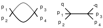
Let us next consider a 1-loop contribution to the four-point vertex function corresponding to the s-channel Feynman diagram in Fig. 17. In the rest of this section, we consider only the continuum limit, and for simplicity we omit a bar to denote the limit.

Calling the s-channel vertex by , we obtain the differential equation
| (197) |
where is part of the tree-level six-point vertex function corresponding to the right diagram in Fig. 18.
Now, satisfies
| (198) |
and the asymptotic condition
| (199) |
since no six-point vertex survives the limit.1515 15 Recall our terminology. Without referring to “asymptotic” behaviors, we can say the same thing as follows. Expanding in powers of and momenta, the leading term is proportional to a negative power of . Hence, the solution is
| (200) |
Substituting this into (197), we obtain
| (201) |
Now, is determined by this differential equation and an additive constant in its asymptotic behavior. To find the asymptotic behavior, we consider the integral
| (202) | |||||
Hence, the asymptotic behavior of is given by
| (203) |
This implies, after summing over three channels,
| (204) |
Now, we obtain
| (205) | |||||
This is integrated to give
| (206) |
The integral on the right-hand side vanishes asymptotically, i.e., as we take and to zero. The additive constant must be zero if we adopt the convention .
3.3 Asymptotic behaviors of the Wilson action and the effective average action
In §2.4 we have introduced the effective average action as the Legendre transform of the Wilson action . Their precise relation is given by (88) and (89). In the continuum limit , let us write for . (We continue omitting a bar to denote the continuum limit.) Then, we can write (88) and (89) as
| (207) |
and
| (208) |
For the interaction parts defined by
| (209) |
we can write (207) as
| (210) |
Since and become equal as , (210) implies that and have the same asymptotic behaviors. In the case of the theory in , the asymptotic behavior (190) of the Wilson action implies1616 16 This is the parameterization adopted in ref. \citenPernici:1998tp, where is denoted as .
| (211) | |||||
3.4 Alternative parameterization
We have shown how to specify the Wilson action of the theory in by specifying by hand. Alternatively, we can specify the behavior of the two- and four-point vertex functions at zero external momentum as an analog of the BPHZ scheme. More concretely, we can impose
| (212) | |||||
| (213) | |||||
| (214) |
for a given choice of the renormalization scale .
Let us see how the above conditions change the choice of at 1-loop. The two-point vertex function becomes
| (215) |
Hence,
| (216) |
Note the non-trivial dependence on .
The four-point vertex function, for a single channel, becomes
| (217) |
where we have used
| (218) |
Hence,
| (219) |
where the factor is for three channels (s,t,u). This also has non-trivial dependence on .1717 17 The non-trivial dependence of on implies that the beta function and anomalous dimension of the squared mass, explained in Appendix B.1, are mass dependent.
In general, a renormalization scheme corresponds to a convention for the coefficients . In Appendix B.2, we will show that changing the three coefficients amounts to changing , and the normalization of under the same renormalization scheme.
4 Composite operators
In this section we introduce composite operators,[17] which provide the most important tool for our program of symmetry realization. By the name we do not mean any random functionals of field variables. Only when a cutoff dependent functional satisfies a particular property, we call it a composite operator.
4.1 Definition
Let be an infinitesimal deformation of a Wilson action so that both and satisfy the same Polchinski equation. Then, the difference satisfies the following linear equation:
| (220) | |||||
This can be rewritten using the interaction part as
| (221) |
In general we call a dependent functional a composite operator if it satisfies the same differential equation as above:
| (222) | |||||
In other words, any dependent functional is a composite operator, if
| (223) |
satisfies the Polchinski equation up to first order in . Note that the right-hand side of (222) is a linear differential operator acting on . Hence, denoting the differential operator by , we may express (222) symbolically as
| (224) |
To determine unambiguously, we must supply either an initial condition at an UV scale , or an asymptotic condition in the case of a renormalizable theory. In the former case, given , we obtain an integral formula for the solution of the differential equation (222) as follows:
| (225) |
This is obtained by taking an infinitesimal variation of the definition (27) of the Wilson action:
| (226) |
If the theory is renormalizable, we can choose the dependence of such that
| (227) |
exists for any fixed . Alternatively, we can impose an asymptotic condition such as
| (228) |
where is the scale dimension of the composite operator , and is the scale dimension of , a product of derivatives of . At a given order in perturbation theory, the coefficient is a polynomial of . If , the dependence of the coefficient of is completely determined by the differential equation (222). For , though, is left ambiguous by an additive constant independent of . Hence, the additive constants , satisfying , parameterize the composite operator. We will give three examples from the theory in in subsect. 4.3. It is important to note that if
| (229) |
for all such that , the operator itself vanishes
| (230) |
due to the linearity of the differential equation (222) and uniqueness of its solution.
To understand the correlation functions of composite operators, let us introduce a source . We recall the relation (33) between and , which can be written in the form of functional integrals as
| (231) |
Changing the action infinitesimally by , the Wilson action changes by . Hence, we obtain
| (232) |
Differentiating this with respect to ’s, we obtain1818 18 As usual, we only consider connected correlations. In the presence of for , we do not factor out the delta function for momentum conservation from the correlation functions.
| (233) |
This is independent of . If the theory is renormalizable, we can take to obtain the continuum limit
| (234) |
where denotes the continuum limit of .
We now wish to show that (231) is equivalent to (226) as we have promised in §2.2. In other words, the relation (231), between the generating functionals and , is equivalent to the definition (226) of the Wilson action; taking an infinitesimal change of and , we obtain (232) from (231), and (225) from (226). Since we have already derived (231) from (226), we only need to derive (226) from (231). For this purpose we use the functional Fourier inverse:
| (235) |
where (or its Fourier transform in real space) is integrated along the imaginary axis. Using (231) to rewrite the right-hand side, we obtain
| (236) |
The integral over is gaussian, and we obtain
| (237) |
This gives (226).
To recapitulate, we have introduced three equivalent criteria for a functional to be a composite operator:
4.2 General examples
We introduce some general examples of composite operators that play important roles in realization of symmetry.
4.2.1
First of all, note that the elementary field is not a composite operator. But
| (238) | |||||
is. We can check this directly by differentiating this with respect to and using the Polchinski equation. Alternatively, we differentiate (231) with respect to to obtain
| (239) |
Since
| (240) |
we obtain
| (241) |
Thus, is a composite operator according to (232). Taking the limit , we obtain that has the asymptotic behavior
| (242) |
For any , we find
| (243) |
is independent of .
4.2.2
Another example is
| (244) |
To see this is a composite operator, we multiply (231) by . An analog of (240) gives, for ,
| (245) |
Combining this with (240), we obtain
| (246) |
Hence, according to (232), (244) is a composite operator. This composite operator may be called the equation of motion operator, since
| (247) |
where is omitted on the right-hand side.
4.2.3
We find
| (248) |
Hence,
| (249) |
is a composite operator, since it is a sum of two composite operators.
4.2.4
We next consider an arbitrary composite operator and the corresponding bare operator so that the two are related by (232). Multiplying this by , and integrating by parts as in (240) and (245), we obtain
| (250) |
Hence, according to (232),
| (251) |
is a composite operator.
The correlation functions of is given in terms of those of :
| (252) |
where is absent on the right-hand side. Divided by , this becomes independent of .
We may call a generalized equation of motion operator, since gives the equation of motion operator .
4.2.5
Suppose that the Wilson action depends on a classical external field , which is not necessarily coupled linearly to the field , so that we may not have an explicit formula such as (41). We find that the derivative with respect to the external field
| (253) |
is a composite operator, since the derivative can be regarded as an infinitesimal deformation of the Wilson action. We indeed find that
| (254) |
is independent of . Hence, substituting into (251), we obtain
| (255) |
is a composite operator. The composite operators and which play important roles for realization of symmetry are given in this form. (See sects. 5 & 7.)
4.2.6
4.2.7 Summary
To summarize, we have introduced the composite operators of the following types:
| composite operator |
|---|
| defined by (238) |
| , the equation of motion |
| , a linear combination of the above two |
| , generalized equation of motion |
| , for an arbitrary external source |
4.3 Composite operators defined by their asymptotic behaviors
In this subsection, we give three concrete examples specifically from the theory in . Since the theory is renormalizable, we can introduce composite operators by specifying their asymptotic behaviors.
- (i)
is defined by the differential equation (222) and the asymptotic condition
(258) The normalization is determined by the value . For example, we can take
(259) If we choose , then the operator vanishes identically.
- (ii)
The dimension operator with zero momentum has the following asymptotic behavior
(260) where parameterize the operator. As a simplest choice, we can take
(261) - (iii)
A related composite operator can be defined by
(262) If we choose , the operator vanishes.
Any scalar composite operator of dimension with zero momentum is given as a linear combination
| (263) |
where the coefficients are independent of .
4.4 1PI composite operators
We recall from §4.1 that a composite operator is an infinitesimal change of the interaction action . Let be the corresponding infinitesimal change in the effective average action . Using the general relations (77) and (83), we obtain
| (264) |
where is given by (89)
| (265) |
We immediately notice that , which has been introduced for the Legendre transformation, coincides with the composite operator defined by (238):
| (266) |
Since and are identical asymptotically, we find that in renormalized theories and have the same asymptotic behaviors:
| (267) |
where is fixed for , and for .
The dependence of for fixed can be obtained easily from the Wetterich equation (112). Varying the effective average action infinitesimally by , we obtain
| (268) | |||||
where we have used the following formula for an infinitesimal variation:
| (269) |
The simplest example satisfying the above differential equation is
| (270) |
for which the right-hand side of (268) vanishes. has no dependence as a functional of ; regarding this as a functional of , however, this has non-trivial dependence as given by (265).
5 Realization of symmetry by WT identity
5.1 WT identity in the continuum limit
In the continuum limit, the Ward-Takahashi (WT) identity for continuous symmetry is given in the following form:
| (271) |
where is a composite operator, giving an infinitesimal symmetry transformation of the elementary field .
We wish to realize the above WT identity in the ERG formalism as an invariance of the Wilson action. Denoting by a composite operator that gives in the continuum limit, we consider an infinitesimal transformation of the elementary field as
| (272) |
As we will explain shortly, the change of the Wilson action under the above transformation is given by the WT composite operator:
| (273) |
This is a composite operator of type (251), integrated over momentum . Hence, its correlation functions are given by
| (274) |
Therefore, the WT identity is equivalent to the vanishing of the WT composite operator :
| (275) |
The WT operator (273) is easy to understand. The first part of
| (276) |
denotes the change of the Wilson action under the infinitesimal transformation (272). The second part
| (277) |
denotes the contribution of the transformation (272) to the jacobian. Hence, (273) is the “quantum” change of the Wilson action, and (275) amounts to the quantum invariance.
Let us consider further. This is determined by and . Recall how and are determined in renormalizable theories. The interaction part of the Wilson action is determined by the Polchinski equation
| (278) |
and its asymptotic behavior. For example, for the theory in , the Wilson action is specified uniquely by the additive constants in the asymptotic behavior:
| (279) | |||||
Similarly, the composite operator is determined by the ERG linear differential equation:
| (280) |
and its asymptotic behavior:
| (281) |
where , and is a local polynomial of and its derivatives.1919 19 may also contain a product of mass parameters such as of the theory. is completely determined by for those satisfying .
Let be the generic parameters of the Wilson action, and be those of the composite operator , so that the theory has altogether parameters that we can adjust. We call the theory symmetric if we can adjust these parameters so that
| (282) |
Note that itself is a composite operator that satisfies the linear ERG differential equation. So, if we show
| (283) |
then it vanishes for any finite .
Let us go over perturbative construction. We expand the parameters in the number of loops:
| (284) |
Let us also expand and in loops:
| (285) |
Suppose is made to vanish up to -loop
| (286) |
by adjusting also up to -loop. Under this assumption, we consider if we can make vanish by choosing appropriately.
Due to the induction hypothesis, satisfies the ERG differential equation
| (287) |
Since for fixed momentum
| (288) |
we find that the right-hand side vanishes and that is independent of for large :
| (289) |
where is independent of , and is a local polynomial of and its derivatives.2020 20 may contain a product of mass parameters such as of the theory which has scale dimension . The scale dimension of must be the same as that of .
On the other hand, from the definition (273), we obtain
| (290) | |||||
Only the first integral depends on the -loop parameters . The dependence is linear. Asymptotically, neither nor has dependence. Hence, the part of that depends on are independent of . For large , the dependence of the first integral cancels that of the second integral, and we find that of (289) is written as the sum
| (291) |
Here, is linear in ’s and ’s with -independent constant coefficients:
| (292) |
denotes the contribution from the second integral of (290), and is determined only by the lower loop coefficients.
Whether or not we can choose ’s and ’s so that
| (293) |
must be examined case by case, and cannot be answered in general. In §6, we discuss four concrete examples. In the cases of QED, the Wess-Zumino model, and the two dimensional O(N) non-linear sigma model, we can prove the possibility of realizing (293). In the case of YM theories we can also satisfy (293), but the possibility cannot be proven within the present formalism; we must resort to the antifield formalism of §7. In general, if a symmetry present at the tree level cannot be extended to arbitrary loop levels, we call the symmetry anomalous. The anomaly is expressed by the non-vanishing . We discuss how the axial and chiral anomalies arise in the ERG formalism in §9.
5.2 WT identity for the bare action
In the previous subsection we have discussed the Wilson action in the continuum limit, and shown how to satisfy the Ward-Takahashi identity by adjusting renormalized parameters. The symmetry is checked with the Wilson action, but not with the correlation functions, which correspond to the Wilson action in the limit of . The advantage of our method is twofold:
- 1.
No problem with massless theories — Low momentum modes are crucially important for the manifestation of the underlying symmetry of the theory. But they are totally irrelevant to the question of the existence of the underlying symmetry. By keeping the cutoff non-vanishing, we stay away safely from the low momentum modes. Massless theories cause no problem, since we never look at the correlation functions.
- 2.
Only a few parameters to deal with — We examine the vanishing of the composite operator for large . The existence of symmetry is a matter of adjusting a few parameters, if it is possible.
In the following we ask if it is possible to realize symmetry using the bare action with a large cutoff . Under the symmetry transformation
| (294) |
the bare action changes by
| (295) |
If the symmetry exists, the above must vanish. Since we are only interested in the continuum limit, we only demand to vanish in the continuum limit . But what does it mean that vanishes in the limit?
Unless it vanishes identically, it is very difficult to see if vanishes or not. To see if it vanishes, we must lower the cutoff from to a finite , and take the limit while fixing . In other words, we must look at , defined by
| (296) |
and check if we can make it vanish in the limit .
In realizing symmetry in the continuum limit, it is difficult to use the bare action and bare WT operator . To appreciate this difficulty, let us consider a bare operator
| (297) |
in the theory in . Naively, this operator appears to vanish in the limit . But that is false. Lowering the cutoff from to , we obtain the following 1-loop correction to :
| (298) |
where
| (299) |
This does not vanish even in the limit . Hence, the small coefficient proportional to in is misleading.
Thus, in general it is difficult to judge the existence of symmetry from the bare action and its transformation property, unless the bare action is exactly invariant, i.e., the symmetry is manifest. We must lower the cutoff from to a finite fixed value . We have already pointed out the potential problem with choosing . Thus, we advocate the examination of symmetry using a Wilson action at non-vanishing .
6 Examples
In this section we give a few examples to apply the formalism introduced in the previous section and realize symmetry as the WT identity (275).
6.1 QED
The WT identities of QED have been discussed using the ERG formalism in various references such as \citenBonini:1993kt, Pernici:1997ie, Sonoda:2007dj to name only a few. Our presentation here follows closely that of \citenSonoda:2007dj.2121 21 For scalar QED, the ERG formalism was first applied in \citenReuter:1994sg.
The classical action of QED is given by
| (300) | |||||
where is a gauge fixing parameter, and are the free Faddeev-Popov ghost, antighost fields. The action is invariant under the classical BRST transformation:
| (301) |
where is an arbitrary anticommuting constant. In the following we quantize this system using the ERG formalism.
The Wilson action of QED is given as the sum of free and interacting parts:
| (302) |
where the free action is given by
| (303) | |||||
Here, we have chosen the same cutoff function for all the fields; it is for the sake of simplicity, and by no means necessary. The cutoff propagators are given by
| (304) |
The ghost and antighost fields are free, and the interaction action depends only on . The Polchinski equation is given by
| (305) |
where the minus sign before the second integral is due to the Fermi statistics. The asymptotic behavior of is given in the following form:
| (306) | |||||
Hence, the theory has 7 parameters:
| (307) |
Out of these, three are unphysical, since they only change normalization of the fields and the mass parameter . So, we can arbitrarily impose the normalization condition
| (308) |
This leaves us four arbitrary parameters:
| (309) |
We will show how to fix these for the theory to become QED.
The quantum BRST transformation is defined by
| (310) |
where is the gauge coupling. We have introduced an anticommuting constant so that the transformation preserves the statistics of the fields. The composite operators , , are defined by
| (311) |
The corresponding WT composite operator is
| (312) | |||||
For the Wilson action to be invariant under the BRST transformation (310), this must vanish.
Substituting the transformation (310) into the above, we obtain2222 22 It is straightforward and not tedious.
| (313) |
where
| (314) |
is a composite operator of type (249), and denotes an electric current. is a composite operator of type (251) defined by
| (315) |
Thus, the WT identity is equivalent to the operator identity:
| (316) |
for arbitrary . This equation is valid if and only if the asymptotic behaviors of the both hand sides match.
The asymptotic behavior of the left-hand side is obtained from (306) as
| (317) | |||||
To obtain the asymptotic behavior of , we first note that vanishes at due to the fermion number conservation. For , substituting the definition of the composite operators, we obtain
| (318) |
Since contains the same number of ’s and ’s, this vanishes:
| (319) |
Therefore, is a total derivative. Hence, its asymptotic behavior must be proportional to . Since has dimension , the most general form is given by
| (320) | |||||
It is crucial that this has the same form as the asymptotic behavior of .
Thus, the WT identity is equivalent to the following four equations:
| (321) |
where we have used the normalization condition . If the right-hand sides do not depend on , we can use the above equations to determine these parameters.
To show that the above equations can be solved uniquely, we must examine the asymptotic behavior of further. Splitting the action into the free and interaction parts, we can rewrite
| (322) | |||||
where
| (323) |
It is straightforward to obtain the asymptotic behavior of the first integral on the right-hand side:
| (324) |
Since by the normalization condition, we find that the above contributes to , and nothing at all to .
We now introduce the loop expansions of the coefficients:
| (325) |
where each term of the series is a function of and . The sum is over 1- and higher-loop contributions; we have fixed the tree level of to satisfy the WT identity (321) at tree level.
Now, let us suppose we have fixed up to -loop level by the WT identity (321). This fixes up to l-loop level. Using this, we can compute (322) up to (l+1)-loop level, where the extra loop is provided by the integral over for the second integral. Then, using (321), we can determine unambiguously. We can repeat this procedure to all orders. This is how we can construct QED perturbatively.
We end this subsection by giving concrete 1-loop calculations. We need to evaluate the second integral on the right-hand side of (322). We only need the tree level vertex and the definition (323) of for the calculations.
- (i)
— The corresponding Feynman graph is given by Fig. 19.

Figure 19: The broken curve gives (323). (326) Using the integral formula (168), we obtain
(327) We also obtain
(328) which is a constant dependent on the choice of .
- (ii)
— The corresponding Feynman graph is given by Fig. 20.

Figure 20: The solid curve gives a high-momentum photon propagator. (329) where the first minus sign is due to the interchange of and . Hence, we obtain
(330) - (iii)
— The corresponding Feynman graph is given by Fig. 21.

Figure 21: The solid line gives a high-momentum electron propagator. Writing , we obtain
(331) Hence, we obtain
(332)
It is interesting to note the presence of . The first and second are photon mass terms, and the third is a four-photon coupling. These break the invariance of the action under the classical BRST transformation (301). As has been emphasized in §5, the theory has full gauge (or BRST) invariance, but it requires order-by-order fine tuning, and is not realized manifestly.
6.2 Yang-Mills theories
In the ERG framework YM theories have been discussed usually in the antifield formalism explained in §7. We give relevant references at the beginning of §8.2.
The classical action of a generic YM theory is given by
| (333) |
where the field strength is defined by
| (334) |
and the covariant derivative is defined by
| (335) |
is a totally antisymmetric structure constant of whatever gauge group under consideration, satisfying the Jacobi identity
| (336) |
The classical action is invariant under the following classical BRST transformation:
| (337) |
where is an arbitrary anticommuting constant. Transforming twice, we obtain
| (338) |
The last one vanishes by the ghost equation of motion
| (339) |
In the following we quantize the system using the ERG formalism.2323 23 We can make the classical BRST transformation nilpotent by introducing an auxiliary field , equal to by the equation of motion. We do not do it here because does not help the perturbative construction described here and in §8.2. In §11, however, we introduce in order to keep the bare action at most linear in the antifields.
The Wilson action is given as the sum of free and interacting parts:
| (340) |
where the free action is given by
| (341) | |||||
Hence, the cutoff propagators are given by
| (342) |
The Polchinski equation for the interaction action is given by
| (343) |
The possible asymptotic behavior depends on the gauge group. For simplicity we consider only the group SU(2). For SU(2), the structure constant becomes the familiar antisymmetric symbol , where the indices run from to . It satisfies
| (344) |
The asymptotic behavior of the interaction action is now given in the following form:
| (345) | |||||
Note that the action depends only on the derivative of the antighost field ; this property certainly holds for the tree level action, and it is further inherited by the Wilson action, since the property is preserved by the Polchinski equation. Hence, besides the gauge coupling , the theory has 7 parameters:
| (346) |
At tree level, we obtain
| (347) |
and the rest vanishing.
Let us now consider the quantum BRST transformation, given by
| (348) |
where the composite operators are defined as usual:
| (349) |
We define the composite operator so that gives the composite operator for the ghost equation of motion:
| (350) |
This is equivalent to
| (351) |
This implies that the asymptotic behavior of is determined by that of the action:
| (352) |
On the other hand, the asymptotic behavior of the composite operator is not determined by the action, and it is given by
| (353) |
The parameter , which is at tree level, is the normalization constant of . This makes the eighth parameter of the theory, besides the seven parameters (346). We wish to fix these eight by demanding the invariance of the Wilson action under the BRST transformation (348). Here, we note that the gauge invariance is expected to leave three parameters free to choose: are the normalization constants of the gauge and ghost fields, respectively, and normalizes the coupling constant . Whatever constraints we find among the eight parameters must leave these three parameters free.
Before going further, let us take a moment to understand the requirement (350). The WT identity for the two-point function is
| (354) |
which gives
| (355) |
Thus, (350) gives
| (356) |
implying that the longitudinal part of the gauge boson propagator does not receive any radiative correction.
The WT composite operator[66] is now defined by
| (357) | |||||
This is a dimension scalar composite operator with ghost number . Hence, for SU(2), its asymptotic behavior must have the following form:
| (358) | |||||
where the coefficients depend on and the gauge coupling constant . As a composite operator, has ten parameters:
| (359) |
We must make these vanish by arranging the eight parameters.
Substituting the BRST transformation (348) into (357), we can simplify the expression of somewhat:
| (360) | |||||
Each of the three integrals is a composite operator by itself.
Let us now introduce loop expansions of and :
| (361) |
Correspondingly, let us expand the parameters:
| (362) |
Suppose we have made
| (363) |
by arranging . Then, as ’s at -loop are all constants, independent of , as a consequence of the ERG differential equation for . We ask if we can choose the -loop coefficients to make all vanish at -loop, which is equivalent to
| (364) |
Examining the structure of above, we find that at -loop the coefficients are given as the sum:
| (365) |
where ’s are linear in ’s, and ’s are determined by the action only up to -loop. Not all ’s are independent; only the following five are independent:
| (366a) | |||||
| (366b) | |||||
| (366c) | |||||
| (366d) | |||||
| (366e) | |||||
The remaining ’s are given by
| (367a) | |||||
| (367b) | |||||
| (367c) | |||||
| (367d) | |||||
| (367e) | |||||
It is possible to make all by adjusting ’s if and only if ’s satisfy the same relations as ’s. If ’s and ’s satisfy the above relations, so do ’s:
| (368a) | |||||
| (368b) | |||||
| (368c) | |||||
| (368d) | |||||
| (368e) | |||||
If these relations hold, we have five linearly independent conditions on eight parameters, leaving three of them arbitrary. This is as expected, since the YM gauge symmetry does not constrain the normalization of fields and the coupling constant . For example, we can adopt the normalization condition:
| (369) |
It is impossible to derive the five relations (368) within the formalism of the WT identity. We will resort to the antifield formalism of §7 for derivation.
6.3 Wess-Zumino model
The ERG formalism has been applied to the Wess-Zumino model, for example, in \citenBonini:1998ec, \citenPernici:1998ex, and \citenRosten:2008ih, where the supersymmetry transformation is linearized via auxiliary fields. Without the auxiliary fields, the supersymmetry transformation is non-linear, and the model was first formulated with ERG in \citenSonoda:2008dz.
The Wess-Zumino model[120] is the simplest supersymmetric model defined in 4 dimensions. Without auxiliary fields, the classical action of the model is given as
| (370) |
where are 2-component spinors, and we define
| (371) |
This is invariant under the following supersymmetry transformation:
| (372) |
where are anticommuting constant spinors.
The above classical action has a spontaneously broken invariance. To make the symmetry manifest, we shift the scalar fields as follows:
| (373) |
Denoting
| (374) |
we can rewrite the action with manifest invariance:
| (375) | |||||
Under the transformation, the fields transform as follows:
| (376) |
In terms of the shifted scalar fields, the supersymmetry transformation is given by
| (377) |
The classical action is parameterized by two complex parameters and . If we ask if their phases have any physical significance, we immediately see that their phase changes can be canceled by the corresponding phase changes of the fields:
- 1.
, are canceled by
(378) - 2.
, are canceled by
(379)
Hence, the physics of the model depends only on and , and we make sure that this property is carried over upon quantization.2424 24 The following results in this section are taken from a recent unpublished work of H. Sonoda and K. Ülker. The use of the symmetry makes the construction much simpler than that given in the earlier work of the same authors [110].
We now consider the Wilson action:
| (380) |
where the free action is
| (381) |
For generality we take the cutoff functions of the bosons and fermions independent, since their equality is not demanded by supersymmetry.
The interaction action is determined by the ERG differential equation
| (382) | |||
and the asymptotic behavior
| (383) | |||||
Hence, the action has six parameters:
| (384) |
We have included as a parameter, even though it corresponds to an additive constant to the action. With the constant term, the derivative of the action with respect to gives an integral of the composite operator
| (385) |
over space:
| (386) |
Similarly, the derivative with respect to gives
| (387) |
The asymptotic behavior (383) implies the following asymptotic behavior of the two composite operators in coordinate space:
| (388) |
We now define the WT identity for supersymmetry by
where the composite operators , etc., are defined by
| (389) |
Under the phase changes of , the composite operator remains invariant, if we change the phases of the fields according to (378) & (379), and at the same time change the phases of according to
| (390) |
In the remainder of this subsection, we wish to show that we can satisfy the WT identity
| (391) |
by tuning four of the six parameters, leaving and arbitrary. The physical meaning of the arbitrary parameters is clear:
- 1.
— overall normalization of the fields; the relative normalization of and is fixed by supersymmetry.
- 2.
— normalization of .
Note that the relative normalization of and is fixed by supersymmetry. Hence, the relative normalization of and is also fixed, since is the derivative of the action with respect to .
We first enumerate all possible terms in the asymptotic behavior of the composite operator :
We have enumerated all terms of dimension up to , which are invariant under the simultaneous phase changes of the parameters and fields given by (378), (379), (390).
At tree level, we find that the choice
| (392) |
satisfies the tree level WT identity
| (393) |
We now assume the vanishing of up to -loop level:
| (394) |
Then, the ERG differential equation for becomes
| (395) |
This vanishes as . Hence, we obtain that
| (396) |
and that ’s are independent of . In the following we wish to show that we can choose so that
| (397) |
We split ’s into ’s linear in ’s and ’s independent of them:
| (398) |
The coefficients ’s can be calculated from
| (399) | |||||
We then obtain, by simple substitution of the asymptotic behavior of & into the above, the following results:
| (400) |
Thus, we must choose ’s so that
| (401) |
For arbitrary ’s, this is solved by
| (402) |
where and remain arbitrary. With the above choice we can make
| (403) |
We end this subsection by giving the results of 1-loop calculations. For simplicity, we take
| (404) |
For the interaction action, we obtain
| (405) |
The coefficients ’s can be calculated from
| (406) |
as follows (Fig. 22):
| (407) |
If we choose
| (408) |
then we obtain
| (409) |

6.4 O(N) non-linear sigma model
The first application of the ERG formalism to the two-dimensional O(N) non-linear sigma model was done by Becchi [17]. The discussion here follows a recent unpublished work by Lütfüoğlu and Sonoda.2525 25 The ERG formalism has been applied to the supersymmetric non-linear sigma models extensively in \citenHigashijima:2002mh,Higashijima:2003rp,Higashijima:2005qk, Higashi:2007ie.
The classical action of the two-dimensional O(N) non-linear sigma model is given by
| (410) | |||||
where the index runs from to , the repeated indices are summed, and
| (411) |
The classical action is invariant under the following infinitesimal rotation:
| (412) |
where are arbitrary infinitesimal constants, and
| (413) |
is the N-th component of an N-dimensional unit vector whose -th component is .
Note that the usual IR problem with the massless scalar does not arise here, since the Wilson action is constructed by integration of high momentum modes . Hence, we do not need to introduce a mass term (or an external field) to break the symmetry explicitly to O(N1).
The Wilson action is given by
| (414) |
where the free action is given by
| (415) |
Hence, the cutoff propagator is
| (416) |
The interaction action is defined by the Polchinski equation
| (417) |
and the asymptotic behavior
| (418) | |||||
where the coefficient functions can be expanded in powers of as
| (419) |
The series for starts from , since the would correspond to a total derivative in the action. At tree level, we find
| (420) |
The infinitesimal transformation is given by
| (421) |
where the composite operator is the composite operator corresponding to the classical . satisfies an ERG differential equation, and is specified by the asymptotic behavior
| (422) |
where the function can be expanded as
| (423) |
At tree level, we find
| (424) |
Thus, the action is parameterized by two functions:
| (425) |
while the transformation is parameterized by a function
| (426) |
Each Taylor coefficient of is a parameter of the Wilson action. Similarly, parameterizes the transformation. Hence, there are an infinite number of parameters. We wish to show how the WT identity determines the three functions.
The WT composite operator is defined by
| (427) |
This has the following asymptotic behavior:
| (429) | |||||
We would like to fine-tune the three functions so that
| (430) |
We prove this possibility by mathematical induction on the number of loops.
Let us introduce loop expansions using the by now familiar notation
| (431) |
Suppose we have determined (or equivalently , ) and (equivalently ) so that
| (432) |
Then, the asymptotic behavior of is independent of , and we can write it as
| (434) | |||||
where are functions of , independent of .
The definition of gives
| (435) |
where
| (436) | |||||
| (437) |
Only depends on , and are determined by and up to -loop.
Therefore, the functions are given as the sum
| (438) |
where are linear in , and are determined by the lower loop functions. We obtain explicitly
| (439) | |||||
| (440) | |||||
| (441) | |||||
where the primes denote derivatives with respect to . There is no relation among the ’s. Thus, whatever ’s are, we can solve the equations
| (442) |
Using
| (443) |
the solution is obtained as follows:
| (444) | |||||
| (445) | |||||
| (446) | |||||
Note that
| (447) |
are left undetermined as constants of integration. This is expected, since normalizes the coupling , normalizes the field , and normalizes the composite operator . For example, we can adopt the convention
| (448) |
or equivalently
| (449) |
This concludes our perturbative proof of the existence of the O(N) non-linear sigma model.
Before concluding this example, let us compute and . (Note by the above convention.) For this, we compute the asymptotic behavior of
| (450) |
up to third order in ’s. The two relevant Feynman diagrams given in Fig. 23.

Note that the two graphs in Fig. 24 give only the terms, but no contribution to the coefficients.

Ignoring the terms, we obtain
| (451) | |||||
up to third order in ’s. Hence,
| (452) |
This gives
| (453) |
6.5 The axial symmetry with a massive propagator
We consider a Wilson action for the spin field:
| (454) |
where the mass is non-vanishing. The free part of the action breaks the axial symmetry explicitly. Nevertheless, the breaking can be compensated by , and the theory can still possess the axial symmetry.
In the presence of the axial symmetry, the correlation functions in the continuum limit satisfy the following WT identity:
| (455) |
The WT operator for the U(1) axial symmetry is given by
| (456) | |||||
where
| (457) |
are the composite operators corresponding to . We can further rewrite the above as
| (458) | |||||
This must vanish for the axial symmetry.
In the simplest case, the theory is free, and the Wilson action is quadratic:
| (459) |
Substituting this into , we obtain the Ginsparg-Wilson relation[47]:
| (460) |
The right-hand side is non-vanishing only for if we choose for . Expanding
| (461) |
with scalar coefficients, the above relation gives
| (462) |
Moreover, the Polchinski equation for gives
| (463) |
which implies
| (464a) | |||||
| (464b) | |||||
To obtain a general solution, we cheat a little. In this case we know the general solution for the continuum limit:
| (465) |
where is a scalar function, independent of .2626 26 We assume parity. Using
| (466) |
we obtain
| (467) |
Hence,
| (468) | |||||
Inverting this, we obtain
| (469) | |||||
This gives
| (470a) | |||||
| (470b) | |||||
which satisfy both the Polchinski equation (464) and the Ginsparg-Wilson relation (462). For small and large momenta, behaves as
| (471) |
For the simplest case
| (472) |
we obtain
| (473) | |||||
In the above, we have seen that the Wilson action of a fully interacting theory must satisfy (458) (or its analog), which reduces to the GW relation (460) only for free theories. However, it is possible to build up a fully interacting theory starting from (460).[58, 64] Particular solutions of (458) that correspond to interacting theories have been constructed explicitly in \citenIgarashi:2002bs,Igarashi:2002ba.
7 Realization of symmetry in the antifield formalism
The purpose of this section is to introduce a method of symmetry realization more powerful than the WT identity discussed in the previous two sections. The method is an adaptation of the antifield formalism of Batalin and Vilkovisky[16, 49, 51] to the ERG formulation of field theory.[62, 61, 60, 63] We introduce only what is needed for perturbative construction of theories, postponing more general discussions till §10. Most results of this section were first obtained by Becchi.[17]. Our presentation here follows §§6,7 of \citenBecchi:1996an.2727 27 For a formulation with the effective average action, see \citenPernici:1997ie, for example.
7.1 Quantum master equation
We introduce an external source in order to generate the symmetry transformation2828 28 The symmetry can be any continuous symmetry, either local or global. For the application of the BV formalism to global symmetries, see Refs. \citenBrandt:1996uv,Brandt:1997cz for example. of as the functional derivative of the Wilson action with respect to . Following the general method by Batalin and Vilkovisky, we give the statistics opposite to that of . In what follows, we treat as a generic bosonic field (scalars and vectors) and as the corresponding fermionic antifield. Extension to a fermionic field and its bosonic antifield is straightforward.
In the antifield formalism, the transformation of is called the BRST transformation,2929 29 For YM theories, this BRST transformation coincides with the ordinary BRST transformation in the limit of vanishing antifields. and it is given as the derivative of the Wilson action with respect to the corresponding antifield:
| (474) |
To show the presence of antifields explicitly, we use a bar above the Wilson action and other related quantities. At the vanishing antifields, the above transformation reduces to the infinitesimal transformation for the WT identity. The WT composite operator is generalized to the quantum master operator
| (475) |
which reduces to the WT composite operator at . Note that is a composite operator. (Quick proof) is a composite operator of type (253). Hence, is a composite operator of type (251).
We now replace the WT identity by the quantum master equation:
| (476) |
which reduces to the WT identity at the vanishing antifields. The quantum master equation implies, for the correlation functions, the following identities:
| (477) |
Given a functional in general, we define its quantum BRST transformation by
| (478) | |||||
This definition is obtained from by changing infinitesimally by . For example, we obtain
| (479) |
so that we can write
| (480) |
The first term is the change of under the infinitesimal field transformation , and the second term is the jacobian.
Suppose is a composite operator. Then,
| (481) |
is a composite operator of type (251). We then note that
| (482) |
is a composite operator of type (257). Since
| (483) |
is also a composite operator, if . If , is not a composite operator in general.
Note also that if , we can rewrite
| (484) |
for an arbitrary functional , not necessarily a composite operator. Since
| (485) |
is a fermionic differential operator acting on the functionals of and , its square vanishes:
| (486) |
Thus, we obtain the nilpotency:
| (487) |
if .
To summarize, the quantum master equation (476), i.e., , implies the following:
- (i)
is a composite operator, if is.
- (ii)
is nilpotent, .
As an example of (i), we find, under the assumption ,
| (488) |
which is a composite operator.
Finally, we come to an important algebraic identity
| (489) |
This simply follows from the definitions (475) of and (478) of . The identity is valid no matter what is. Eq. (489) is the algebraic structure we have been missing in our discussion of the WT identity in §5. We will see, in §7.2, how useful this identity is for the realization of continuous symmetry in the ERG approach.
7.2 Outline of perturbative construction
We now outline a perturbative construction of the theory that satisfies the quantum master equation (476). Let us first introduce loop expansions:
| (490) |
If the theory is renormalizable, the asymptotic behavior of the Wilson action is given in the form
| (491) |
where is a local polynomial of , and their derivatives, and is the scale dimension of . The Wilson action is parameterized only by that has . We introduce the loop expansion of as
| (492) |
Our starting point is the classical action which is independent of the cutoff . Since the interaction part of the tree level action is the sum of tree graphs consisting of the vertices of and high-momentum propagators, we obtain
| (493) |
We assume that this satisfies the classical master equation:
| (494) |
Since is the asymptotic part of , we obtain
| (495) |
Now, our induction hypothesis is
| (496) |
For this we have adjusted the parameters of the theory up to -loop order. In other words we have adjusted
| (497) |
Since is a composite operator satisfying the ERG differential equation, the induction hypothesis implies that is independent of for large . In the following we wish to show that we can fine-tune so that
| (498) |
which is equivalent to
| (499) |
Hence, (498) completes the perturbative construction by mathematical induction.
To show the possibility of such fine-tuning, we must examine the structure of further:
| (500) | |||||
where
| (501) | |||||
| (502) |
For large , is independent of . Hence, the dependence of and must cancel for large . Note that only depends on , and is completely determined by the lower loop parameters.
For later convenience, we introduce the following notation. We first denote
| (503) |
We then denote the independent part (namely the part that does not vanish at ) of the asymptotic behavior of by so that
| (504) |
Similarly, we denote the independent parts of and by , , respectively. In defining these, we ignore the part multiplied by positive powers of either or . By definition, we obtain
| (505) |
Now, for large , (501) gives
| (506) |
Introducing the classical BRST transformation
| (507) |
we can rewrite the above as
| (508) |
The classical master equation (494) implies the nilpotency of the classical BRST transformation:
| (509) |
Hence, we obtain
| (510) |
We now consider the algebraic identity (489). At -loop, this gives
| (511) |
due to the induction hypothesis (496). Considering large , we obtain
| (512) |
This gives
| (513) |
To summarize so far, our goal is to show that we can fine-tune the -loop parameters so that . This condition is equivalent to solving
| (514) |
where
- 1.
- 2.
satisfies (513), i.e., closed under .
- 3.
is given by (504), the most general local functional of fields with dimension .
Thus, we have converted the problem of perturbative construction into a question of classical algebra.3030 30 This is called the BRST cohomology. For (514) to have a solution, it is sufficient that implies ; using a more proper mathematical language, the BRST cohomology defined by must be trivial.
The final algebraic question (514) does not have any general solution. The answer depends on the the set of available fields and antifields and the choice of the classical action . But it is clear what we must do. We first consider the most general that satisfies (513), using the available set of fields and antifields. If it can be given as , the theory can be constructed. If not, the symmetry is anomalous, and we cannot construct a symmetric quantum theory based on the classical action.
8 Examples
8.1 QED
In §6.1 we have already shown how to construct QED with the help of a WT composite operator. Though we do not need the antifield formalism for assurance of the theory’s existence, it is instructive to see how the formalism applies to QED.
Our starting point is the classical action:
| (515) |
where is given by (300). Here, the fields with the superscript ∗ are antifields that have the opposite statistics to the respective conjugate fields. Let us tabulate them:
| field | antifield | statistics | dimension |
|---|---|---|---|
| Fermi | |||
| Bose | |||
| Bose | |||
| Bose |
The classical action satisfies the following classical master equation:
| (516) |
Except for the term quadratic in , the antifield dependence of the action is determined so that the derivative of the action with respect to the antifield gives the BRST transformation of the corresponding field:
| (517) |
We note that all the antifields are coupled linearly to the dynamical fields. The are coupled to the quadratic fields , respectively, but these are basically linear since the free field acts almost like an external field.
Let us consider the dependence of the Wilson action on each antifield.
- (i)
— This is coupled linearly to , contributing a term
(518) to the Wilson action. Since is free, no further dependence is generated.
- (ii)
— The linear coupling
(519) amounts to an external source
(520) coupled linearly to the gauge field . From the general result (41), the linear coupling generates the quadratic term:
(521) Furthermore, the shift
(522) is generated in the interaction part of the Wilson action.
- (iii)
— We can regard the free field as part of the external source coupled to :
(523) Hence, from the general result (41), we find first that the quadratic term
(524) is generated, and second that the fields are shifted as
(525) in .
Altogether, we obtain the following action in the presence of antifields:[65][53]
| (526) | |||||
where is the free part defined by (303), and is the interaction part constructed in §6.1. The fields are shifted in the interaction part. If , without shifts, satisfies the Polchinski equation for QED, so does given above.3131 31 In §11.1, we rederive this result using a functional method.
We now wish to show that thus constructed indeed satisfies the quantum master equation. The quantum master operator is defined by
| (527) | |||||
We now substitute (526) into the above to express it in terms of . We skip the intermediate steps which are long but straightforward.3232 32 The details of a similar calculation are given for the O(N) linear sigma model in Appendix E. Toward the end, we use the anticommuting nature of :
| (528) |
for any symmetric integration kernel . We finally obtain the result
| (529) |
where is the WT composite operator of QED defined in §6.1, and the fields are shifted as (522) and (525). Since for arbitrary field variables, we obtain
| (530) |
8.2 YM theories
For YM theories, the antifield formalism is essential for proving the possibility of their construction. We recall, from §6.2, that we still have to derive the algebraic relations (368), necessary in order to show the possibility of realizing by fine-tuning the parameters. The first application of the ERG formulation and antifield formalism was done by Becchi[17]. This work was extended subsequently in \citenBonini:1993sj,Bonini:1994dz,Bonini:1994kp,Bonini:1995tx,Bonini:2000wr among others. Our presentation here follows closely §7 of Ref. \citenBecchi:1996an with quite a few additions for pedagogy.[109]
In the presence of the antifields, the classical action is given by
| (531) | |||||
For convenience, we tabulate the antifields below:
| field | antifield | statistics | dimension | ghost number |
|---|---|---|---|---|
| Fermi | ||||
| Bose | ||||
| Bose |
The ghost numbers are assigned so that the action has zero ghost number. The classical action satisfies the classical master equation:
| (532) |
As in the case of QED, the BRST transformation of a field is given by the functional derivative of the classical action with respect to the conjugate field:
| (533) |
We now consider the Wilson action in the presence of antifields. As in QED, we can determine the dependence of the Wilson action on and . Let us consider them one by one:
- (i)
— This antifield is coupled linearly to the gauge field as
(534) This generates the quadratic term
(535) and the shift
(536) in the interaction part of the Wilson action. This dependence on is the same as in QED.
- (ii)
Now that we have determined the dependence on and , the Wilson action has the following form:
| (540) |
where is given by (341), and
| (541) | |||||
reduces to the Wilson action of §6.2 for the vanishing antifields. Especially, we find
| (542) |
The interaction action is determined by the Polchinski equation
| (543) | |||||
and an asymptotic behavior. For SU(2), the latter is given in the following form:
| (544) | |||||
We note that all the coefficients are the same as in §6.2; as for , they survive the limit of zero antifields, and as for , we must find
| (545) |
Hence, the introduction of the antifields does not increase the number of parameters of the theory. We still have the same eight parameters
| (546) |
at our disposal.
Now, the quantum master operator is defined by
| (547) | |||||
This reduces to the WT composite operator (357) of §6.2 at the vanishing antifields. We wish to fine-tune the eight parameters (546) to make vanish. The possibility of such fine-tuning can be proven if we can derive the algebraic constraints (368).
The derivation of (368) takes some steps. We first rewrite the quantum master operator using all we know about the antifield dependence of . Substituting (540) and (541) into the definition (547), we obtain
| (548) | |||||
where we define
| (549) |
and
| (550) | |||||
Note that the quadratic kinetic term of the gauge field in is purely transverse. Hence, depends only on the following combinations of the field variables:
| (551) |
Therefore, shifting and its antifield by terms proportional to , we define a modified quantum master operator by
| (552) |
where is for the shifted variables, and defined by
| (553) | |||||
Then, the quantum master equation
| (554) |
is equivalent to the modified quantum master equation
| (555) |
It is the modified action (553) and the corresponding quantum master operator (552) that we apply the general formalism developed in §7. Let us identify the classical algebraic problem corresponding to (514):
| (556) |
First, the classical action is given by
| (557) |
which satisfies the classical master equation
| (558) |
Then, the classical BRST transformation is defined by
| (559) |
which is nilpotent
| (560) |
due to the classical master equation. The most general form of , for SU(2), is given by
| (561) | |||||
where we use the familiar notation for the loop expansion
| (562) |
Now, is a dimension fermionic scalar composite operator of ghost number . Hence, the most general form of is given by
| (563) | |||||
where are constants. Replacing by , this is the same as the asymptotic behavior of in the absence of the antifields. (See (358).) Similarly, and are parameterized by and , respectively, instead of . Then,
| (564) |
implies
| (565) |
Since
| (566) |
is determined by ’s. But is determined only by the lower loop parameters.
Let us consider ’s. (566) gives
| (567a) | |||||
| (567b) | |||||
| (567c) | |||||
| (567d) | |||||
| (567e) | |||||
and
| (568a) | |||||
| (568b) | |||||
| (568c) | |||||
| (568d) | |||||
| (568e) | |||||
These are the same results as (366) & (367) that we have found in §6.2.
Next, we consider ’s. The algebraic constraint
| (569) |
implies
| (570a) | |||||
| (570b) | |||||
| (570c) | |||||
| (570d) | |||||
| (570e) | |||||
These are the relations that were missing in §6.2.
Thus, gives only five independent equations
| (571) |
The solution is given by
| (572a) | |||||
| (572b) | |||||
| (572c) | |||||
| (572d) | |||||
| (572e) | |||||
where we have treated the normalization constants as independent parameters. The simplest choice is to set them zero for .
9 Axial and chiral anomalies
In this section we formulate the axial and chiral anomalies in the ERG formalism. We restrict our discussions only to abelian anomalies, and it suffices to use only the WT identity of §5. The anomalies have been computed in the ERG formalism in Refs. \citenBonini:1997yv,Bonini:1994xj, \citenPernici:1997ie, but here we follow an unpublished work by Igarashi, Itoh, and Sonoda. For references, we would like to mention that the chiral anomalies have been studied using the antifield formalism (but not ERG) in \citenTroost:1989cu, \citenDeJonghe:1993zc, and using the BRST cohomology (but not ERG) in \citenBarnich:1994ve,Barnich:1994mt,Barnich:1994db,Barnich:2000zw.
9.1 Axial anomaly in QED
In the following we wish to consider the axial vector current in QED, and compute its divergence
| (573) |
To define the axial vector current precisely, it is convenient to couple an external field to the axial vector current. In the Wilson action, we only consider up to first order. introduces the following extra terms into the asymptotic behavior of the action:
| (574) |
where we have suppressed the terms independent of . We define the axial vector current as the composite operator:
| (575) |
This has the asymptotic behavior
| (576) | |||||
The parameter normalizes the axial vector current, and the ratio is determined by the WT identity of QED as we will see shortly. The above asymptotic behavior implies
| (577) | |||||
To determine , we consider the WT identity in the presence of . In §6.1 we have found that the WT identity is given by
| (578) |
The two composite operators are defined by
| (579) |
and
| (580) | |||||
In the presence of , the asymptotic behaviors of both and get an extra term linear in :
| (581) | |||||
| (582) |
where the terms independent of are suppressed. Thus, the gauge invariance requires
| (583) |
We leave open the convention for the normalization constant of the axial vector current for later convenience.
We now consider the composite operator of type (251) at :
| (584) | |||||
This has the correlation functions:
| (585) |
The asymptotic behavior of has the following form:3434 34 is a pseudo scalar even under charge conjugation. Hence, the dimension pseudo scalars , are forbidden.
| (586) | |||||
To rewrite , we introduce two composite operators:
- (i)
with the asymptotic behavior
(587) where we choose the convention
(588) - (ii)
with the asymptotic behavior
(589) We will make a convenient choice for shortly.
We can now expand
| (590) |
where are independent constants, dependent only on and . The right-hand side has the asymptotic behavior
| (591) | |||||
Comparing this with (586), we obtain
| (592) |
where we have used (583). By adopting the convention
| (593) | |||||
| (594) |
we obtain
| (595) | |||||
| (596) | |||||
| (597) |
Hence, we obtain
| (598) |
The last term gives the axial anomaly. We will show the 1-loop calculations of the axial anomaly in the next subsection. From (626, 628), setting , we obtain
| (599) |
so that the coefficient of the axial anomaly is
| (600) |
9.2 Chiral anomaly
9.2.1 gauge theory
Let us try to construct a gauge theory with massless fermions. Its classical action is given by
| (601) | |||||
where
| (602) |
This action is invariant under the following classical BRST transformation:
| (603) |
where is an arbitrary anticommuting constant.
The quantization follows the same line as for QED. We omit writing down the Polchinski equation for the interaction action . Its asymptotic behavior is given in the following form:
| (604) |
Here the terms are new features, not present in QED. Given is a vector, and is an axial vector, we find that the terms are allowed by parity. (Note and are forbidden by parity.)
We define the quantum BRST transformation by
where the composite operators in the square brackets are defined as usual.
The corresponding WT composite operator is given by
| (612) | |||||
Substituting the above BRST transformation, we can rewrite this as
| (613) |
where the composite operators are defined by
| (614) |
and
| (615) | |||||
| (616) | |||||
where the matrix is defined by (323) with :
| (617) |
In the following we examine the asymptotic behavior of the WT composite operator . We will restrict our discussion to the part relevant to chiral anomalies, i.e., the part proportional to the tensor. The asymptotic behavior (604) implies
| (618) |
We have only one parameter at our disposal.
On the other hand, assuming parity, the asymptotic behaviors (only the part proportional to the tensor) of are expected to be of the following form:
| (619) |
Thus, for , we need to find
| (620) |
If this is the case, we can make vanish by choosing
| (621) |
Let us compute at 1-loop. Only the second integrals of (615) and (616) contribute.
- (i)
— The term of is given by the Feynman diagram in Fig. 25 and the one with and interchanged.

Figure 25: A Feynman diagram contributing to . The broken line gives . The graph gives the integral
(622) where is defined by (617). Its limit can be calculated as follows:
(623) Finally, using
(624) we obtain
(625) The other graph gives the same contribution, and altogether we obtain
(626) - (ii)
— The term of is given by the diagram in Fig. 26, similar to the previous diagram.

Figure 26: The broken line gives . The difference is in the use of instead of , and replacement of by . There is one more graph obtained by interchanging and . The graph in Fig. 26 gives
(627) The other graph gives the same. Hence, we obtain
(628) - (iii)
— The term of can be calculated similarly. We obtain
(629)
Thus, we find
| (630) |
No matter what we choose as , we cannot satisfy . At best, we can save the vector gauge invariance by choosing
| (631) |
This leaves us the following chiral anomaly:
| (632) | |||||
9.2.2 gauge theory
We construct a quantum theory whose classical action is given by
| (633) |
where and are chiral:
| (634) |
For the quantum theory, the WT composite operator is given by
| (635) |
where
| (636) | |||||
where is defined by (617). has the asymptotic behavior
| (637) | |||||
Compared with for QED, has an extra term proportional to the tensor. On the other hand, the asymptotic behavior of has the same form as for QED:
| (638) | |||||
which implies
| (639) | |||||
Hence, unless
| (640) |
by chance, we cannot satisfy the Ward identity by adjusting the parameters in hands.
At 1-loop, the coefficient can be calculated from Fig. 25 where is replaced by , and is multiplied by the projection operator from the left. We obtain
| (641) | |||||
where is replaced by . There is another graph with and interchanged. Hence, we obtain
| (642) |
Therefore, we cannot satisfy the WT identity.
10 Functional integral approach to the antifield formalism
In §§7 & 8 we have adapted the antifield formalism to the ERG framework. Though our discussion has been limited to perturbation theory, we have obtained an important conclusion: realization of symmetry is reduced to solving a classical algebraic problem. The purpose of the present section is to give a second look at the adaptation of the antifield formalism without relying on perturbative expansions.
The antifield formalism of Batalin and Vilkovisky[16][49][51] can provide us with a systematic description of any symmetry present in a theory. In the following we apply the antifield formalism to the bare and Wilson actions. The quantum master equation (QME), satisfied by an action, signals the presence of symmetry, naturally extending the WT identity discussed in §5. As opposed to §§7 & 8, where we have constructed the continuum limit directly, we start from a bare action at a UV scale . Following the procedure of §2 we construct a Wilson action by integrating the fields over the momenta between and (). With kept finite, the resulting ERG trajectory approaches the trajectory of the continuum limit only as . (See Fig. 16.) Nevertheless, by keeping finite, we can manage to write down more explicit expressions for the antifield dependence of the Wilson action,[65, 53, 67] compared with the perturbative construction in terms of the asymptotic behavior in §§7 & 8.
We discuss only a generic gauge theory in this section, and give concrete examples in the next section. A global symmetry can be treated in a similar manner,[64][59] though we do not discuss it here.3535 35 The QME for chiral symmetry is an extension of the well-known Ginsparg-Wilson relation.[47] In §6.5 we have briefly discussed the WT identity for the axial symmetry. The organization of this section is as follows. In §10.1, we first review the classical antifield formalism, and then explain the modification necessary for quantized systems. For classical systems a symmetry is realized as a classical master equation (CME), and for quantum systems as a quantum master equation (QME). We then show, in §10.2, how to adapt the formalism in the presence of a UV cutoff, and in §10.3, how the QME relates to the WT identity. In §10.4 we derive explicit antifield dependence of the Wilson action, assuming a simple form for the BRST transformation of the bare action. In §10.5 we introduce the effective average action, and rewrite the QME for the Wilson action as the so-called “modified Slavnov-Taylor identity”[40] for the average action. Finally, in §10.6 we discuss an implication of the nilpotency of the BRST transformation.
In this section, we adopt a notation that can handle bosonic and fermionic fields equally in order to respect the canonical structure of the antifield formalism. We use the symbol with a suffix for fields, and distinguish their statistics by Grassmann parity mod :
| (643) |
Though not mentioned explicitly in §§7 & 8, a field and its corresponding antifield form a canonical pair. In order to keep the canonical structure, we rescale an antifield by the cutoff function . Hence, we must replace the antifield of the previous sections by to get the corresponding results in this section.
10.1 The Batalin-Vilkovisky antifield formalism
Let us consider a classical gauge fixed action that is invariant under the nilpotent BRST transformation :3636 36 The right (left) derivative is indicated by the superscript ().
| (644) |
The fields represent collectively gauge and matter fields as well as (anti)ghosts and B-fields.3737 37 The field is an auxiliary field which is equal to the divergence of the gauge field by the equation of motion. We introduce this to avoid the quadratic term in (645). The index represents any index to distinguish different types of fields, such as momentum, the Lorentz index for a vector field, and the spinor index for a spinor field. Hence, the Einstein convention for repeated includes integration over momenta.
By introducing an antifield for each field , we define an extended action
| (645) |
The antifield has the opposite Grassmann parity to that of :
| (646) |
We also assign ghost numbers to and so that they add up to .
In the space of and , we define a canonical structure by introducing an antibracket: for any field variables and , we define
| (647) |
Fields and their antifields are canonical conjugate pairs, satisfying
| (648) |
We now define the BRST transformation of an arbitrary variable by
| (649) |
This generalizes for the fields ; for example, it gives the transformation of antifields by
| (650) |
Following the definitions (645), (647), (649), we obtain
| (651) |
where is defined by (644). Hence, if (644), and the original BRST transformation is nilpotent
| (652) |
we obtain the classical master equation (CME):
| (653) |
Thus, CME is equivalent to the combination of the BRST invariance of (644) and the nilpotency (652). In fact the nilpotency of the BRST transformation (649) remains valid, even if acts on an arbitrary variable , dependent on both and ; applying twice, we obtain
| (654) |
Hence, (653) implies the general nilpotency:
| (655) |
We now apply the BV formalism to quantum systems with BRST invariance. Let be an action that defines a quantum system via functional integration over : is either a bare action with a UV cutoff , or a Wilson action with a lower cutoff . Under the BRST transformation of fields
| (656) |
the action changes by the quantum master operator:
| (657) |
where we define
| (658) |
The first term is the classical change of the action under the BRST transformation (656). The second term is the contribution from the jacobian of the BRST transformation. The system is BRST invariant quantum mechanically if the two contributions cancel:
| (659) |
We call this equation the quantum master equation (QME). Note that the quantum master operator (657) appears somewhat different from (475); the cutoff dependent factor is missing in (657). This is due to the adoption of a different normalization of the antifields, as mentioned in the last paragraph before §10.1.
In the antifield formalism, we define the quantum BRST transformation as
| (660) |
for an arbitrary variable . Without assuming QME, we obtain two important identities:
| (661) | |||
| (662) |
These identities are algebraic, consequences of the definitions of the quantum master operator (657) and the quantum BRST transformation (660). The identity (661) is crucial for the perturbative construction of symmetric theories, as shown in §§7 & 8. Eq. (662) implies that the quantum BRST transformation (660) is nilpotent if and only if QME (659) holds. Note the importance of the second term in (660). If we defined the BRST transformation without it by
| (663) |
we would obtain
| (664) |
and hence nilpotency demands CME instead of QME. For a generic quantum system, however, what holds is QME, but not CME. Therefore, it is the quantum BRST transformation that can be nilpotent.
10.2 Scale change in the functional integral approach
The action of the previous subsection is either a bare action or the corresponding Wilson action .3838 38 As in §2 we denote a bare action by and a Wilson action by . As in §§7 & 8 we also put a bar to denote the dependence on antifields. We recapitulate the important results of §2 using the notation adopted in the present section.
Let be an action defined at the UV scale in the presence of antifields:
| (665) |
where is the sum of the gaussian and interaction terms:
| (666) |
Here, we have adopted the matrix notation for momentum integrals:
| (667) | |||||
| (668) |
We have assumed that the antifield dependence of is strictly linear.
By introducing sources , we define the generating functional
| (669) |
In performing the above functional integral, we decompose the fields into the IR fields and UV fields , where the propagators of each class of fields are given by
| (670) |
Note that carry the momenta below , and those between and .
We now introduce the Wilson action[65][65]
| (671) |
where the interaction part is defined by the functional integral over the UV fields :
| (672) |
The two antifields are related simply as
| (673) |
We define the generating functional of the Wilson action by
| (674) |
The two generating functionals (669) and (674) are related by (33), which is rewritten as
| (675) |
where the normalization factor is given by
| (676) |
Because of its importance, we wish to rederive it using the present notation. The main tool is the triviality of the gaussian integral:
| (677) |
We substitute this into the partition function defined by (669), and perform a canonical change of variables from to , where
| (678) |
Then, we obtain
| (679) | |||||
where is given by (676). This is independent of the antifields , and we may adopt a gauge choice
| (680) |
This gives
| (681) |
We will justify this relation shortly. With the above gauge choice, we obtain (675) & (676), where the Wilson action is defined by (671) & (672).
The partition function does not depend on the IR cutoff so that
| (682) |
This yields the Polchinski differential equation[94]
| (683) |
where we define
| (684) |
as in (51). is completely determined by the Polchinski differential equation and the initial condition
| (685) |
We can define a composite operator as a functional that satisfies the differential equation (224). Using the present notation, we obtain
| (686) |
where
| (687) |
Note that the first term of (687), rescaling of the antifield, is a consequence of (681). Hence, the factor is necessary in order to make
| (688) |
composite operators.
For later convenience, we recall an alternative definition of composite operators. Given an arbitrary functional at the UV scale, the corresponding IR composite operator is constructed as
| (689) |
This implies
| (690) |
in the presence of arbitrary sources coupled linearly to the fields.
10.3 WT identity and QME
In this subsection we consider the cutoff dependence of the quantum master operator. Our starting point is the BRST transformation of fields at the UV scale , given in terms of an anticommuting constant as
| (691) |
In computing the generating functional (669), we consider changing integration variables from to . If the jacobian is properly taken into account, the integral does not depend on the choice of integration variables. Hence, we obtain
| (692) | |||||
where is the WT operator defined by
| (693) |
is the sum of the change of the original gauge fixed action
| (694) |
and the contribution from the jacobian
| (695) |
The quantum master operator defined by3939 39 Note that here is (658), but not the log derivative of .
| (696) |
is indeed given as the sum of the WT operator and the third term of (692):
| (697) |
where we have used . Hence, we obtain a simple relation between the QM and WT operators:
| (698) |
As CME implies both the BRST invariance of the action and the nilpotency of the BRST transformation, QME also implies both. In contrast, the WT identity implies only the invariance of the action.
We now rewrite (692) as
| (699) |
Setting , we obtain an analogous relation for the WT operator:
| (700) |
Using (691), we obtain
| (701) |
where the differential operator is called the Slavnov operator. Setting we obtain
| (702) |
Therefore, we can rewrite (699) and (700) as
| (703) | |||||
| (704) |
We note that the above relations, being based upon the functional relation (692), are valid whether or not the bare action is invariant under the BRST transformation (691).
We now wish to transform (703) into an equivalent condition on the Wilson action . We first apply (689) to define the QM operator for the IR theory by
| (705) |
Then, (690) implies
| (706) |
We also define the IR operator corresponding to by
| (707) | |||||
Eq. (690) implies
| (708) |
Denoting
| (709) |
we can rewrite (708) as
| (710) |
Hence, using (706) and (710), we can transform (703) into
| (711) |
which is the desired relation.
The above relation implies
| (712) |
This has the form expected for the quantum master operator; here the relevant action is the Wilson action defined at an IR scale , and the BRST transformation of the IR field is a composite operator if multiplied by .
Similarly, we can transform (704) into
| (713) |
where the WT operator and the BRST transformation are obtained by setting to zero:
| (714) | |||||
| (715) |
So far our discussion has been kept very general; we have only assumed that the bare action takes the form of (665) & (666). For symmetric theories the QME must hold: and hence must vanish. For renormalizable theories, the QME need not hold for any finite , but it must hold in the limit . In general it is a difficult problem to construct a bare action that satisfies the QME exactly; in §§7 & 8 we have discussed this problem directly in the limit , but only perturbatively. For anomaly-free renormalizable theories, we can exepect that the quantum master operator behaves as
for a large but finite value of .4040 40 We write only to mean that it vanishes as . To be more precise, we expect
| (716) |
or equivalently,
| (717) |
for an arbitrary source .4141 41 Later in eqs. (11.1) and (805), we write explicitly for gauge theories. Thanks to renormalizability, the action has only a finite number of parameters. Our assumption is that we can tune the parameters so that eq. (716) holds. This is the statement of the BRST invariance of the bare theory defined at the UV scale . As a consequence of (706), the QME for the Wilson action is given either as
| (718) |
or
| (719) |
Before concluding this subsection, we consider a particular class of BRST transformation
| (720) |
which are at most quadratic in fields. The BRST transformation for QED and YM theories belongs to this class. We wish to obtain an explicit expression for the corresponding IR composite operator . In order to rewrite the expectation value
for the IR theory, we need to compute two things.
First, we compute the first order differential:
| (721) | |||||
where we define
| (722) | |||||
Second, we compute the second order differential:
| (723) | |||||
where we define
| (724) | |||||
Note that nontrivial contributions arise from derivatives acting on the normalization factor .
Hence, using (710), we obtain
| (725) |
Since this is valid for arbitrary , we obtain the operator equality
| (726) |
It is important to mention the necessity of the cutoff function to make (726) UV finite.4242 42 The potential UV divergence is hard to see in the matrix notation. It is hidden in the loop momentum integral contained in .
10.4 Antifield dependence of the Wilson action
In this subsection we derive the general structure of the Wilson action , in particular its dependence on the antifields. We first make some assumptions for the bare action that are general enough to accommodate the cases of QED and Yang-Mills theories. Then, we describe how the Wilson action depends on the antifields. In §11 we will give the Wilson actions for QED and Yang-Mills theories more explicitly.
As for QED, the Wilson action first obtained in ref. \citenHigashi:2007ax has two different types of antifield dependence, one that can be written down explicitly and the other that appears as a linear shift of the field variables by antifields. These features are seen in Eqs. (789)-(791) in the next section.4343 43 Eqs.(789)-(791) differ from those given in ref. \citenHigashi:2007ax, where no UV cutoff is introduced. As for non-Abelian gauge theories, additional non-trivial antifield dependence exists. In this section, we will show how to modify the method of \citenHigashi:2007ax to treat the non-Abelian gauge symmetry. Based on this, we will give explicitly the Wilson action for Yang-Mills theories in (812).
Without losing generality, we assume that the bare action is linear in antifields and the BRST transformation quadratic in fields:
| (727) | |||||
| (728) | |||||
| (729) |
The bare actions of QED and Yang-Mills theories can be given in this form.
The functional integral (672) over the UV fields defines the interaction part of the Wilson action, . We rewrite the integrand of (672) as
| (730) |
where the effective sources coupled to are given by
| (731) |
and
| (732) |
For the terms quadratic in and linear in the antifield, we replace by the derivative . The Wilson action then takes the form
| (733) |
In order to simplify the above further, we follow ref. \citenHigashi:2007ax and introduce a change of variables. First, we complete the square with respect to in the first two terms of the integrand:
| (734) |
where
| (735) |
We then introduce new variables so that :
| (736) |
Finally we obtain
| (737) |
Using the definition of in the absence of antifields
| (738) |
we obtain our final expression for the Wilson action:
| (739) |
With (739) we can construct the action from . The antifield dependence comes partly from (731), and partly from the shifted variables (736). The remaining antifield dependence is solely generated by the exponentiated differential operator in the logarithm. This complicates and the BRST transformation of the fields . Once the antifields are removed, however, we have simple expressions [66]:
| (740) | |||||
where
| (741) | |||||
| (742) | |||||
We can obtain the same results from (726) simply by setting the antifields to zero.
Before closing this subsection, we make a comment on the ghost equation of motion: we wish to point out that the actions for gauge theories depend on the antighost and the antifield through a particular linear combination.
Let us consider the classical action (645) either for QED or for Yang-Mills theories. The gauge-fixing and the ghost parts of are written as[73]
| (743) |
where is a gauge-fixing condition. If we choose the covariant gauge fixing
| (744) |
where is a gauge field, and an auxiliary field, we obtain
| (745) | |||||
Therefore, in , the antifield appears as a linear combination with the antighost, . Hence, the action satisfies
| (746) |
We now assume that the bare action satisfies the same equation:
| (747) |
This implies the same relation for the Wilson action
| (748) |
because and are both composite operators. We call Eqs. (746), (747), (748) the ghost equations of motion. We encountered these before, first as (350) and then as (537). In fact in §8.2, (537) plays an important role in simplifying the perturbative construction of the theory. We will assume (747) and hence (748) when we discuss examples in the next section.
10.5 QME and the modified Slavnov-Taylor identity
In §2.4 we have discussed the relation between a Wilson action and the corresponding effective average action . The two are related by a Legendre transformation. A theory can be constructed equally well in terms of or . As for realization of symmetry, however, we have so far considered only the Wilson action. In this subsection we make a brief detour to write down the identity for , corresponding to the QME for . This is called the modified Slavnov-Taylor identity[40]. We also give a brief note on the same subject as Appendix D. Compared with Appendix D, we employ a more functional method here.
As in §2.4 we introduce an action with both UV and IR cutoffs:
| (749) |
The gaussian term suppresses the momentum modes or . The generating functional is defined by
| (750) |
The Legendre transform of is defined by
| (751) |
where is defined in terms of as
| (752) |
In the following we wish to consider the functional integral over the QM operator for the bare action:
| (753) |
and express this in terms of the effective average action .
As a preparation, we first compute the derivatives of :
| (754) | |||||
| (755) |
Hence, we obtain
| (756) | |||||
where is the QM operator for the action :
| (757) |
To find the difference between and , we note
| (758) |
where we define
| (759) |
Hence, we obtain
| (760) |
The functional integral over the difference gives
| (761) | |||||
where we have used (754), (755). To summarize so far, the functional integral over (760) gives
| (762) | |||||
To further rewrite the second term in the above, we introduce the notation:
| (763) |
where (755) is used. Then, the inverse is written as
| (764) |
Hence, we can rewrite (762) as
| (765) | |||||
Imposing this to vanish, we obtain the modified Slavnov-Taylor identity[40]:
| (766) |
In the limit of , goes to zero and becomes . Therefore, the modified ST identity reduces to the Zinn-Justin equation.
10.6 On the nilpotency without antifields
As shown toward the end of §10.1, the quantum master equation (659) implies the nilpotency of the quantum BRST transformation , defined by (660). Even if is nilpotent, the reduced BRST transformation
| (767) |
that appears in the WT operator (714) is not nilpotent in general. In this subsection we compute , and study how it differs from zero, assuming the nilpotency of the full BRST transformation.
Take a functional of the field defined at an IR scale , and consider its BRST transformation:
| (768) |
Expanding the Wilson action in powers of antifields
| (769) |
we obtain an expansion
| (770) |
Setting , we obtain
| (771) |
By the definition (660), the nilpotency of implies
| (772) |
Setting to zero, the first term on the right gives . Therefore, we obtain
| (773) |
Using the expansions (769) & (770), we obtain
| (774) | |||||
In particular, we obtain
| (775) |
Thus, we have found that fails to be nilpotent in a particular way that is a total derivative, or using the terminology introduced in §4.2, is a generalized equation of motion.4444 44 Note that is not necessarily a composite operator. Hence, we are abusing the terminology introduced for genuine composite operators.
11 Examples: the Wilson actions for QED and Yang-Mills theories
The purpose of this section is to apply the general result (739) on the antifield dependence of the Wilson action to QED and the Yang-Mills theories. As for QED this has already been done in §8.1, from a consideration of the ERG differential equation. This method works only for QED, but not for YM theories. For the latter we have adopted a perturbative approach in §8.2, and have shown how to construct the continuum limit of the Wilson action by loop expansions. In §8.2, we have discussed the antifield dependence of only the asymptotic behavior of the Wilson action, since that is all we need for proving the theory’s existence. In contrast, we have adopted a unifying approach in §10, and have determined the antifield dependence of the Wilson action explicitly by starting from a bare action that has simple antifield dependence.4545 45 The antifield dependence of the bare action is linear in and at most quadratic in as in (729).
11.1 QED
We first consider QED and reproduce the results from \citenIgarashi:2007fw and \citenHigashi:2007ax. Our derivation follows closely that of \citenHigashi:2007ax except that we pay more careful attention to the necessity of a UV cutoff for the bare theory.
Denoting the UV fields by
| (776) |
and the UV antifields by
| (777) |
the bare action of QED is written as follows4646 46 We have introduced the auxiliary field to avoid the quadratic dependence of on . The result (526) is obtained from (801) by integrating out .:
| (778) |
where
and
The coefficients
| (787) |
are given such dependence on that we obtain a finite continuum limit.
Denoting the IR fields and antifields by
| (788) |
the effective sources defined by (731) are given by
| (789a) | |||||
| (789b) | |||||
| (789c) | |||||
| (789d) | |||||
Since the ghost and antighost remain free, and are absent in the interaction action , the source does not appear in the IR action. This simplifies the application of the general result (739). The differential operators, in (739), generate no contribution. The Wilson action is thus given as
| (790) | |||||
where the shifted variables are defined by
| (791a) | |||||
The term quadratic in the effective sources is given by
Hence, the total Wilson action is
| (801) | |||||
Since QED is renormalizable, we can tune the dependence of the bare parameters (787) to obtain the continuum limit of . The remaining dependence of on comes from in the term and the shifted variables . In the limit , is simply replaced by , and we obtain the continuum limit of as in \citenHigashi:2007ax. A canonical transformation that eliminates the quadratic terms in the antifield gives the action obtained in ref. \citenIgarashi:2007fw. Perturbative construction of that satisfies the WT identity, , has already been discussed in §6.1.
11.2 Yang-Mills theories
We consider a Yang-Mills theory without matter described by the UV action4747 47 We suppress the group index and use the notations: and .
| (802) |
where fields and antifields are collectively denoted as
| (803) |
The bare action consists of the kinetic part
| (804) | |||||
and the interaction part
| (805) |
Here, we have assumed the gauge group SU(2) to write down ; more terms are available and need to be introduced for higher symmetry. The coefficients depend on .
The Wilson action with the IR fields & antifields
| (806) |
is given by the general formula (739). Let us get a concrete expression. The effective sources read
| (807a) | |||||
| (807b) | |||||
| (807c) | |||||
and the differential operator w.r.t. is given by
| (808) |
The shifted variables defined by (736) are given by
| (809) |
It is easy to see that does not depend on :
| (810) |
The quadratic term in that appears inside the exponentials of (739) takes the following concrete form:
| (811) |
Putting together the above results, we obtain the Wilson action:
| (812) | |||||
In writing down the bare action (802) we have assumed the ghost equation of motion (747) to hold. Hence, the Wilson action (812) must satisfy (748), i.e., the Wilson action must depend on the antighost and the antifield for the gauge field only through the linear combination, . The way we have written (812) for , this is not manifest.
12 Concluding remarks
We hope we have succeeded in achieving the two goals that we have set in §1. Formulating a field theory with a momentum cutoff is the most natural, and it accords with Wilson’s non-perturbative definition of a field theory. It is still surprising that we can describe the continuum limit using a finite momentum cutoff, but it does not come for free: the cutoff function needs to be smooth, and the Wilson action contains an infinite number of terms. The formalism of ERG is simple enough that we only need several pages to summarize the essence of all done in this review. We have given a quick summary as Appendix F.
We have introduced two ways of realizing continuous symmetry: one with the WT identity, and another with the QME. Among the examples we have discussed in §§6 & 8, only YM theories need the QME for proving the possibility of construction. Let us try to understand this. The WT identity is the invariance of the Wilson action under infinitesimal transformations, and it knows nothing about the algebra formed by the transformations. We need the antifield formalism to incorporate an algebraic structure. Take the example of the two dimensional O(N) non-linear sigma model discussed in §6.4. Commuting two generators that move the N-th axis, we get an element of O(N1), under which the action is manifestly invariant. Take the Wess-Zumino model. Commuting two supersymmetry generators, we get a translation, under which the action is manifestly invariant. Hence, either in the non-linear sigma model or the Wess-Zumino model, the algebra of infinitesimal transformations does not constrain the theory. Hence, the WT identity suffices. This is not the case with YM theories; we need the antifield formalism to incorporate the full algebra of BRST transformations.4848 48 The antifield formalism is necessary only to prove the possibility of perturbative construction. The WT identity suffices for the order-by-order construction.
As for perturbative applications, our list of examples is not exhaustive. Among those missing, supersymmetric YM theories are particularly important. The ERG formalism has been already applied,[35, 6, 23] but our understanding is still incomplete regarding the non-renormalization properties.[104][119] We also think it important to prove the non-renormalization theorem for chiral anomalies using the ERG formalism; to our knowledge it has not been done.
As for non-perturbative applications, the order-by-order solution of the WT identity or QME is inappropriate. Even approximate solutions will do as long as they are given in closed form. Progress along this line is hoped for.
In this review we have been primarily concerned with formulating various symmetric theories. The formalism has matured enough that we are ready to address more physical questions.
Acknowledgment
The authors would like to thank Prof. K. Higashijima for suggestions and encouragement.
Appendix A Generalized diffusion equations
In §2 we have derived a particular ERG differential equation (55) for the interaction part of the Wilson action, , defined by (27). The purpose of this appendix is twofold:
- 1.
to rewrite (27) as a formula that gives the entire Wilson action,
- 2.
This is done by (814), where different choices of correspond to Wilson’s and Polchinski’s ERG differential equations.
In the following we adopt a notation slightly different from that in the main text. We write for , and for , where is defined by
| (813) |
The logarithmic parameter grows, as the momentum cutoff decreases.
A.1 Derivation of the generalized diffusion equations
We consider a one-parameter family of actions for a real scalar field . We generate the -dependence by a gaussian integral transformation of the following type:[124, 121]
| (814) |
We impose the two properties
| (815) |
in order to assure the limit
| (816) |
The two factors and have the following physical meanings:
- 1.
blocking factor — is the Fourier transform of a block spin. Denoting the Fourier inverse of and by the same symbols, we write
(817) Then, the inverse Fourier transform of is the block spin or average field:
(818) The size of the domain of should grow exponentially as .
- 2.
We will shortly give examples of and .

We now wish to derive the differential equation for , analogous to the diffusion equation. We first consider the -derivative:
| (819) | |||||
where we have suppressed the argument of the last exponential. We compare the above with the first and second order functional derivatives of :
| (820) | |||||
| (821) | |||||
where we have ignored an additive constant proportional to the space volume.
Thus, we obtain the generalized diffusion equation
| (822) | |||||
This can be rewritten for as
| (823) | |||||
where
| (824) |
The equation for has the same form as the ERG differential equation (59) for the full action.
We now define the generating functional of the connected correlation functions:
| (825) |
Using the technique familiar from §2.2, we can compute in terms of as follows:
| (826) | |||||
Now, shifting by , we obtain
| (827) | |||||
Hence, we obtain
| (828) |
This means that nothing is lost in going from to ; we can construct from , and vice versa. Differentiating the above equation with respect to , we obtain the following equation for the connected correlation functions:
| (829) |
This is a generalization of (47). Hence, of has the same correlations as the block spin of the original . The smearing factor affects only the two-point correlation function. This is a well known general characteristic of diffusion processes.4949 49 The diffusion equation preserves the connected part of the correlation for .
We now choose a particular blocking function, given in terms of a cutoff function :
| (830) |
where is an anomalous dimension, which affects only the overall normalization of the field. For , we obtain
| (831) |
if we assume for . Hence, the support of the Fourier transform has size in space, growing exponentially as increases. This choice of corresponds to
| (832) |
With the above choice for , we obtain
| (833) | |||||
Hence,
| (834) |
where we impose the initial condition
| (835) |
Let us now look at two examples of and calculate the corresponding .
Example 1 (Wilson)
We choose
| (836) |
This is the original choice of Wilson discussed in sect. 11 of \citenWilson:1973jj.5050 50 We have not introduced rescaling of space. This is discussed briefly in Appendix C. This gives
| (837) | |||||
Hence, we obtain
| (838) |
using the initial condition (835). Thus, using (830), we obtain
| (839) |
This implies
| (840) |
Wilson’s choice is characterized by the following behavior of the two-point function as :
| (841) |
Example 2 (Polchinski)
The Polchinski equation (59) is obtained if we choose , and
| (842) |
Here, we make a slightly generalized choice without assuming :
| (843) | |||||
where is a -dependent squared mass, and
| (844) |
Let us find the corresponding ; we find
| (845) |
Hence,
| (846) |
Thus, we obtain
| (847) |
Hence, we obtain the following dependence of the correlation functions:
| (848) |
and
| (849) |
These reduce to (47) if we take and -independent .
A.2 Extention to fermions
In extending the generalized diffusion equations to fermions, we only consider the spin fields in . We generate the following one-parameter family of actions:
| (850) |
where is a scalar, and & are 4-by-4 matrices. We choose
| (851) |
so that
| (852) |
Let us define the generating functional by
| (853) |
We then obtain the familiar relation
| (854) |
where denotes the inverse of the matrix .
To derive the differential equation for , it is convenient to rewrite
| (855) | |||||
From this, we obtain the following ERG differential equation:
| (856) | |||||
where
| (857) |
Example 1 (Polchinski)
We take
| (858a) | |||||
| (858b) | |||||
Then we obtain
| (859) |
Example 2 (chirality breaking diffusion)
We keep the same blocking factor , but take the smearing factor
| (860) |
so that
| (861) |
The smearing factor breaks chirality explicitly. Even if we start from the chiral invariant action
| (862) |
the diffusion process breaks chiral symmetry explicitly, and is not manifestly chiral invariant. But it does inherit the chiral invariance of the original action , as will be shown at the end of the next subsection. It is straightforward to find
| (863) |
where
| (864) |
This satisfies the initial condition:
| (865) |
Now, we take , while we keep finite. We obtain the continuum limit:
| (866) |
This has an interesting property:
| (867) |
For , chiral invariance becomes manifest.
A.3 WT operator for chiral invariance
As an application, let us formulate the WT identity for chiral invariance. At scale , we define the WT operator
| (868) |
for chiral invariance (axial invariance to be more precise). implies that the action is invariant under the chiral transformation:
| (869) |
We wish to study how the chiral symmetry is realized by the Wilson action with .
A familiar calculation gives
| (870) |
where
| (871) |
Hence, the chiral invariance of is given by
| (872) |
For a free theory5151 51 The quantum master equation and its solutions have been studied for interacting fermions in Refs. \citenIgarashi:2002ba,Igarashi:2002bs,Igarashi:2001cv. See also Ref. \citenIchinose:1999ke
| (873) |
the relation reduces to the Ginsparg-Wilson relation[47]
| (874) |
ERG gives the following -dependence:
| (875) |
Substituting this into the Ginsparg-Wilson relation above, we obtain what is expected:
| (876) |
which is equivalent to
| (877) |
Appendix B Applications of composite operators
In the main text we have shown how to realize symmetry in terms of either a WT composite operator or a QM composite operator . In this appendix we describe two further applications of composite operators: one to beta functions, and the other to universality.
B.1 Beta functions
We recall that the Wilson action of the theory in is defined by the Polchinski equation
| (882) |
and the asymptotic behavior
| (883) | |||||
The Wilson action is parametrized not only by which appears in the differential equation, but also by the three parameters . Here, for the sake of simplicity, we make a simple choice[106]:
| (884) |
We call this the MS scheme for its similarity to the minimal subtraction scheme for dimensional regularization.[112, 111] We immediately notice, though, that the MS scheme depends on the choice of . The MS scheme (884) for a different corresponds to that do not satisfy (884) for the original . It is the purpose of this appendix to derive the dependence of the Wilson action in the MS scheme (884).[108](See also \citenHughes:1987rf,Bonini:1996bk for derivations of beta functions from the ERG. Ref. \citenPernici:1998tp derives the same mass independent RG equation as (903).)
Since can be regarded as a constant external field, the derivative of the Wilson action
| (885) |
is a composite operator. (Here, and are fixed.) To be more precise, it is a dimension composite operator with zero momentum. Hence, it must be a linear combination of the three linearly independent composite operators
| (886) |
which are defined at the end of §4.3. The asymptotic behavior (883) implies the following asymptotic behavior:
| (887) | |||||
where
| (888) |
Hence, we obtain
| (889) |
where the coefficients depend only on .
We now wish to rewrite the above equation as a physically meaningful equation. For this purpose, we construct an alternative basis of dimension composite operators with zero momentum.
We first consider
| (890) |
This is a composite operator of the type (253), since can be regarded as a constant external field. This satisfies
| (891) | |||||
Similarly, we wish to construct a composite operator that gives
| (892) |
for any . For , the derivative of will do:
| (893) |
But, for , we obtain
| (894) |
Hence, we need that satisfies
| (895) |
This is easily constructed as
| (896) |
Hence, we obtain
| (897) | |||||
It is straightforward to check that this satisfies the ERG differential equation (222).
The third and last composite operator is defined by
| (898) |
where
| (899) |
is the composite operator corresponding to . is a composite operator of the type (251), and it has a simple correlation function
| (900) |
for any .
Thus, we have obtained an alternative basis of dimension scalar composite operators with zero momentum, consisting of
| (901) |
We can use this basis, instead of the basis consisting of (886), to expand :
| (902) |
where the coefficients are all functions of alone, since they cannot depend on . The physical meaning of this equation is clear. It implies, for the correlation functions,
| (903) |
This is a mass independent renormalization group equation. [111, 118]
B.2 Universality
Universality is an important concept in renormalization theory. To construct a continuum limit, there are always more than one way. The independence of the continuum limit on the particular method of construction is called universality. For example, if we use a lattice to construct a continuum theory, the limit should not depend on what kind of lattice, whether square or cubic, we use.
In the following we examine universality in two restricted senses. First, we wish to show that the continuum limit (i.e., the correlation functions with the suffix ) does not depend on the particular asymptotic conditions we use to select a solution of the ERG differential equation. Second, we wish to show that the continuum limit does not depend on the choice of a cutoff function .
Scheme dependence
Let us compare two solutions of the same Polchinski differential equation (882). One is satisfying the MS condition (884), and the other is satisfying
| (904) |
where are all infinitesimal constants. Then, is a composite operator given by
| (905) |
Using the alternative basis, we can rewrite this in the form
| (906) |
This implies that , which does not satisfy the MS condition (884), gives the same continuum limit as the Wilson action satisfying (884) with squared mass and coupling . The only difference is in the normalization of fields by a factor . Extending this, we can show that the action with any choice of is equivalent to an action satisfying the MS condition (884) up to field normalization.
Dependence on the choice of
In our discussions so far, we have always kept a choice of the cutoff function . Physics should not depend on the choice of , and we will show this in the following.
Let be a solution of the ERG equation with the cutoff function , infinitesimally different from . We would like to construct an equivalent action that has as the cutoff function. We first recall that the correlation functions in the continuum limit are given by
| (907) |
This can be rewritten as
| (908) | |||||
| (909) | |||||
We now construct a new Wilson action by
| (910) | |||||
This has the correlation functions:
| (911) |
so that
| (912) | |||||
| (913) |
This implies
- 1.
that satisfies the Polchinski equation with the cutoff function ,
- 2.
that gives the same continuum limit as .
Hence, the continuum limit does not depend on the choice of a cutoff function. Note that even if obeys the MS condition (884), does not necessarily obey it.
Appendix C ERG differential equations for fixed points
In the main text we use the Polchinski differential equation, (55) for and (59) for , to construct the continuum limit of renormalizable theories. This equation is NOT what was originally proposed by K. G. Wilson for his non-perturbative studies of field theory [124]. As we lower the cutoff , the cutoff function keeps changing its momentum dependence, and hence the Polchinski equation has no fixed point. In this appendix we explain how to modify the Polchinki equation to obtain an ERG differential equation that can have non-trivial fixed points.
To have a fixed point, we must do two things:
- 1.
make everything dimensionless by multiplying an appropriate power of the cutoff ,
- 2.
rescale the field to normalize the kinetic term.
Let us explain the above one by one:
- 1.
For the real scalar theory in dimensions, the Fourier transform has mass dimension . Using the dimensionless ratio
(914) we define the dimensionless field
(915) We then rewrite the Wilson action
(916) as
(917) where we define
(918) so that
(919) The parameter is a dimensionless parameter such that
(920) If satisfies the Polchinski equation, then satisfies
(921) where we have omitted the bar above the integration variable .
- 2.
To obtain a fixed point, we must normalize the field to satisfy
(922) This further modifies the differential equation to
(923) where the constant , anomalous dimension, is determined as
(924)
The last ERG differential equation (923) has not only the gaussian fixed point
| (925) |
but also a non-trivial fixed point, called the Wilson-Fisher fixed point, if .
In the above we have modified the ERG differential equation not only to have a fixed point, but also to give simple -dependence to the correlation functions, similar to (47). We find the following results:
| (926a) | |||
| (926b) | |||
The original differential equation, given in \citenWilson:1973jj, is based upon Wilson’s ERG differential equation (Example 1 of §A.1), and is somewhat different from the above:
| (927) | |||||
The difference in the second line comes from the choice of (836). In \citenWilson:1973jj, the function is denoted as
| (928) |
Expanding in powers of fields
| (929) |
the anomalous dimension is determined by the normalization condition
| (930) |
as
| (931) |
(927) gives slightly different -dependence to the two-point correlation function:
| (932a) | |||
| (932b) | |||
Appendix D Symmetry of the effective average action
The purpose of this appendix is to rewrite the WT identity and quantum master equation of the Wilson action as those of the corresponding effective average action. We have briefly discussed this in §10.5, where a more functional method is used than the method here. Our main tool is the relation between a composite operator and its 1PI sibling, given by (264) & (265).
We first consider a generic WT composite operator
| (933) |
where is a composite operator of momentum giving an infinitesimal transformation of . The corresponding 1PI composite operator is defined by
| (934) |
where
| (935) |
(In this appendix, we consider only the continuum limit .) Since and coincide asymptotically, and share the same asymptotic behavior.
In order to express in terms of , we consider the two composite operators and one by one.
- (i)
— The corresponding 1PI composite operator is given by
(936) - (ii)
Thus, we obtain
| (940) | |||||
where we have used (101)
| (941) |
and
| (942) |
For example, the WT identity for QED
| (943) | |||||
is rewritten as
| (944) | |||||
where
| (945) |
We next consider the quantum master operator
| (946) |
The antifield is a classical external field, and it does not affect the Legendre transformation between and . The Legendre transformation is given by
| (947) |
where
| (948) |
From the general relation (77), we obtain
| (949) |
Hence, the 1PI quantum master operator is given by
| (950) | |||||
Since
| (951) |
by construction, and share the same asymptotic behavior. For YM theories,
| (952) |
is called the modified Slavnov-Taylor (ST) identity, first obtained by Ellwanger [40].
Appendix E O(N) linear sigma model
In this subsection we apply the antifield formalism to the O(N) linear sigma model. The model is a typical example of theories with their symmetry realized linearly. In such cases, it should not be surprising that the WT identity or the QME for the Wilson action boils down to the invariance of the action under the naïve linear transformation.5252 52 In preparing this appendix, we have benefited from the discussions with Drs. K. Ülker and L. Akant. Though we do not discuss it here, the Wess-Zumino model with auxiliary fields has its supersymmetry linearly realized, and the supersymmetry of the Wilson action is invariant under the naïve linear supersymmetry transformation.[35, 93, 102]
We consider a theory of real scalar fields invariant under the following linear O(N) transformation:
| (957) |
where is an infinitesimal constant. The -by- matrices are real and antisymmetric, and they satisfy the commutation relation
| (958) |
where the structure constants are real and completely antisymmetric, and satisfy the Jacobi identity:
| (959) |
The Wilson action is given as
| (960) |
where the free part is
| (961) |
Using the composite operator corresponding to the elementary field
| (962) |
the WT composite operator is given by
| (963) |
The WT identity
| (964) |
is equivalent to the cutoff independent identities
| (965) |
for any .
We now wish to show that the WT identity (964) is equivalent to the naïve identity:
| (966) |
This is done in two steps. First we show the vanishing of the jacobian:
| (967) |
This vanishes because of the antisymmetry of . Second we consider
| (968) |
where we have used the antisymmetry of again. Hence, the WT identity is equivalent to (966).
We now promote to anticommuting ghost fields, constant in space. We then introduce the fermionic antifields for and bosonic constant antifields for . We define the action by
| (969) | |||||
where the interaction action is the same as before, except that the fields are shifted by antifields:
| (970) |
is constructed so that it satisfies the same Polchinski differential equation as . The last -independent term generates the O(N) transformation of the ghosts:
| (971) |
The QM operator is defined by
| (972) | |||||
We wish to verify that the QME
| (973) |
is equivalent to the WT identity (964), and hence equivalent to the naïve identity (966). Verification is straightforward but takes several steps.
- 1.
We first compute
(974) Hence,
(975) and therefore
(976) by the antisymmetry of .
- 2.
We then compute
(977) - 3.
We therefore obtain
(978) Hence,
(979) - 4.
Using
(980) we obtain
(981) - 5.
We compute
(982) Since
(983) by the Jacobi identity, we obtain
(984) - 6.
We finally obtain the desired relation
(985)
The last relation is already familiar from QED, for which we have derived (529), even though the abelian gauge symmetry of QED is not strictly linear in the sense used here.
To conclude, we have found that for the O(N) global symmetry, the following three equations are equivalent:
| (986a) | |||||
| (986b) | |||||
| (986c) | |||||
The jacobian of the linear transformation is :
| (987) |
Appendix F Quick summary
ERG
- 1.
A cutoff function and its log derivative :
(988) We usually (not always) choose
(989) - 2.
The interaction part of the Wilson action satisfies the Polchinski equation
(990) - 3.
The full Wilson action
(991) satisfies the ERG differential equation
(992) - 4.
Under the initial condition , the integral solution of the Polchinski equation is given by
(993) - 5.
For renormalizable theories, can be determined by the Polchinski equation and its asymptotic behavior:
(994) For the theory in , we choose
where the coefficients are determined by the Polchinski equation up to
(995) which constitute the renormalized parameters of the theory. A particularly simple choice is
(996) - 6.
No loss of information along the ERG flow: the correlation functions
(997) are independent of .
- 7.
is a composite operator if satisfies the ERG differential equation to first order in , or equivalently if satisfies the differential equation
(998) Given an initial condition , the integral formula for is
(999) - 8.
The independent correlation functions of a composite operator:
(1000) - 9.
Examples of composite operators
- (a)
(Equation of motion)
(1001) - (b)
, where is an external source.
(1002) - (c)
has the asymptotic behavior
(1003) - (d)
If is a composite operator, so is
(1004) (1005) - (e)
If is a composite operator, so is
(1006) (1007)
- (a)
- 10.
For the theory in , the composite operator is determined by the differential equation and the asymptotic behavior
(1008) where is an arbitrary normalization constant.
Ward-Takahashi (WT) identity
- 1.
Under the symmetry transformation of the field
(1009) where is a composite operator, the Wilson action changes by
(1010) The WT composite operator is a composite operator of type (d).
- 2.
The WT identity is given by
(1011) Since is a composite operator,
(1012) guarantees the WT identity for all .
- 3.
The WT identity is equivalent to
(1013)
Quantum master equation
- 1.
We generalize the Wilson action to by introducing an antifield , conjugate to . has the opposite statistics to . is a classical external source that generates the transformation of .
- 2.
The quantum master operator
is a composite operator of type (d), since is a composite operator of type (e).
- 3.
The quantum master equation
(1014) is satisfied, if
(1015) - 4.
The quantum master equation is equivalent to the WT identity
(1016) - 5.
The Wilson action , deformed by the composite operator , satisfies the quantum master equation, if and only if
(1017) where the BRST transformation is defined by
(1018) - 6.
For any composite operator , is a composite operator if . Then,
(1019) For example,
(1020) satisfies
(1021) - 7.
The algebraic identity
(1022) even if .
- 8.
The nilpotency needs the QME .
Classical nature of the quantum master equation
- 1.
Loop expansions (bars omitted; , etc.)
(1023) Loop expansions of the asymptotic parts:
(1024) - 2.
induction hypothesis: Given that satisfy , we wish to construct so that
(1025) This condition is equivalent to
(1026) - 3.
Tree level: we start from the classical action with the classical BRST invariance
(1027) We then choose
(1028) so that
(1029) - 4.
Under the induction hypothesis, the ERG differential equation
(1030) implies that is independent of .
- 5.
satisfies the differential equation
(1031) We split into two parts:
(1032) - (a)
is independent of , not determined by the differential equation.
- (b)
is a particular solution of the differential equation for .
We wish to fine tune so that .
- (a)
- 6.
We split into two parts:
(1033) where
- (a)
implies is independent.
- (b)
is independent, and so is .
- (a)
- 7.
is equivalent to
(1034) - 8.
The classical BRST transformation is defined by
(1035) This is nilpotent:
(1036) - 9.
Since
(1037) we obtain
(1038) - 10.
and the induction hypothesis imply
(1039) Taking the asymptotic form, we obtain
(1040) Hence, implies
(1041) - 11.
is equivalent to
(1042) - 12.
Thus, we must prove the triviality of the cohomology of :
(1043)
References
- [1] M. G. Alford, \PLB336,1994,237.
- [2] K.-I. Aoki, \IJMPB14,2000,1249.
- [3] K.-I. Aoki, Non-perturbative renormalization group approach to dynamical chiral symmetry breaking in gauge theories in *Nagoya 1996, Perspectives of strong coupling gauge theories*, (1996) 171, hep-ph/9706204.
- [4] K.-I. Aoki, K.-I. Morikawa, W. Souma, J.-I. Sumi, and H. Terao, \PTP95,1996,409.
- [5] K.-I. Aoki, K.-I. Morikawa, W. Souma, J.-I. Sumi, and H. Terao, \PTP99,1998,451.
- [6] S. Arnone, C. Fusi, and K. Yoshida, \JHEP02,1999,022.
- [7] S. Arnone, Y. A. Kubyshin, T. R. Morris, and J. F. Tighe, \IJMPA17,2002,2283.
- [8] S. Arnone, T. R. Morris, and O. J. Rosten. \JLEur. Phys. J., C50,2007,467.
- [9] C. Bagnuls and C. Bervillier, \PRP348,2001,91.
- [10] R. D. Ball and R. S. Thorne, \JLAnn. Phys.,236,1994,117.
- [11] R. D. Ball, P. E. Haagensen, J. I. Latorre, and E. Moreno, \PLB347,1995,80.
- [12] G. Barnich, F. Brandt, and M. Henneaux, \CMP174,1995,57.
- [13] G. Barnich, F. Brandt, and M. Henneaux, \CMP174,1995,93.
- [14] G. Barnich, F. Brandt, and M. Henneaux, \PRP338,2000,439.
- [15] G. Barnich and M. Henneaux, \PRL72,1994,1588.
- [16] I. A. Batalin and G. A. Vilkovisky. \PLB102,1981,27.
- [17] C. Becchi, On the construction of renormalized gauge theories using renormalization group techniques, hep-th/9607188.
- [18] F. Benitez, J.-P. Blaizot, H. Chaté, B. Delamotte, R. Méndez-Galain, and N. Wschebor, arXiv:0901.0128 [cond-mat.stat-mech].
- [19] F. Benitez, R. Méndez Galain, and N. Wschebor, \PRB77,2008,024431.
- [20] J. Berges, N. Tetradis, and C. Wetterich, \PRP363,2002,223.
- [21] C. Bervillier, B. Boisseau, and H. Giacomini, \NPB801,2008,296.
- [22] C. Bervillier, B. Boisseau, and H. Giacomini, \NPB789,2008,525.
- [23] A. Bilal, \ANN323,2008,2311.
- [24] M. Bonini, M. D’Attanasio, and G. Marchesini, \NPB409,1993,441.
- [25] M. Bonini, M. D’Attanasio, and G. Marchesini, \PLB329,1994,249.
- [26] M. Bonini, M. D’Attanasio, and G. Marchesini, \NPB421,1994,429.
- [27] M. Bonini, M. D’Attanasio, and G. Marchesini, \NPB418,1994,81.
- [28] M. Bonini, M. D’Attanasio, and G. Marchesini, \NPB437,1995,163.
- [29] M. Bonini, M. D’Attanasio, and G. Marchesini, \PLB346,1995,87.
- [30] M. Bonini, M. D’Attanasio, and G. Marchesini, \NPB444,1995,602.
- [31] M. Bonini, G. Marchesini, and M. Simionato, \NPB483,1997,475.
- [32] M. Bonini and E. Tricarico, \NPB585,2000,253.
- [33] M. Bonini and E. Tricarico, \NPB606,2001,231.
- [34] M. Bonini and F. Vian, \NPB511,1998,479.
- [35] M. Bonini and F. Vian, \NPB532,1998,473.
- [36] F. Brandt, M. Henneaux, and A. Wilch, \PLB387,1996,320.
- [37] F. Brandt, M. Henneaux, and A. Wilch, \NPB510,1998,640.
- [38] F. De Jonghe, hep-th/9403143.
- [39] B. Delamotte, cond-mat/0702365v1 [cond-mat.stat-mech].
- [40] U. Ellwanger, \PLB335,1994,364.
- [41] U. Ellwanger, M. Hirsch, and A. Weber, \JLZ. Phys. C69,1996,687.
- [42] M. E. Fisher, \JLRev. Mod. Phys., 70, 1998, 653.
- [43] F. Freire, D. F. Litim, and J. M. Pawlowski, \IJMPA16,2001,2035.
- [44] F. Freire and C. Wetterich, \PLB380,1996,337.
- [45] F. Freire, D. F. Litim, and J. M. Pawlowski, \PLB495,2000,256.
- [46] H. Gies, hep-ph/0611146.
- [47] P. H. Ginsparg and K. G. Wilson, \PRD25,1982,2649.
- [48] G. R. Golner, hep-th/9801124.
- [49] J. Gomis, J. Paris, and S. Samuel, \PRP259,1995,1.
- [50] A. Hasenfratz and P. Hasenfratz, \NPB270,1986,687.
- [51] M. Henneaux and C. Teitelboim, Quantization of Gauge Systems (Princeton University Press, 1992).
- [52] T. Higashi, K. Higashijima, and E. Itou, \PTPS164,2007,103.
- [53] T. Higashi, E. Itou, and T. Kugo, \PTP118,2007,1115.
- [54] K. Higashijima and E. Itou, \PTP108,2002,737.
- [55] K. Higashijima and E. Itou, \PTP110,2003,563.
- [56] K. Higashijima and E. Itou, hep-th/0511300v1.
- [57] J. Hughes and J. Liu, \NPB307,1988,183.
- [58] I. Ichinose and K. Nagao, \JLChin. J. Phys., 38, 20000, 671.
- [59] Y. Igarashi, M. Ishikake, K. Itoh, H. Sawanaka, and H. So, \JPA39,2006,8023.
- [60] Y. Igarashi, K. Itoh, and H. So, \IJMPA16,2001,2047.
- [61] Y. Igarashi, K. Itoh, and H. So, \PTP104,2000,1053.
- [62] Y. Igarashi, K. Itoh, and H. So, \PLB479,2000,336.
- [63] Y. Igarashi, K. Itoh, and H. So, \PTP106,2001,149.
- [64] Y. Igarashi, K. Itoh, and H. So, \PLB526,2002,164.
- [65] Y. Igarashi, K. Itoh, and H. Sonoda, \PTP118,2007,121.
- [66] Y. Igarashi, K. Itoh, and H. Sonoda, \PTP120,2008,1017.
- [67] Y. Igarashi, K. Itoh, and H. Sonoda, Quantum master equation for yang-mills theory in the exact renormalization group in preparation.
- [68] Y. Igarashi, H. So, and N. Ukita, \PLB535,2002,363.
- [69] Y. Igarashi, H. So, and N. Ukita, \NPB640,2002,95.
- [70] G. Keller and C. Kopper, \CMP148,1992,445.
- [71] G. Keller and C. Kopper, \CMP153,1993,245.
- [72] G. Keller, C. Kopper, and M. Salmhofer, \JLHelv. Phys. Acta, 65, 1992, 32.
- [73] T. Kugo and S. Uehara, \NPB197,1982,378.
- [74] O. Lauscher and M. Reuter, Quantum Einstein gravity: Towards an asymptotically safe field theory of gravity, volume 721 (Springer Berlin / Heidelberg, 2007).
- [75] D. F. Litim, \PRD64,2001,105007.
- [76] D. F. Litim, arXiv0810.3675 [hep-th].
- [77] D. F. Litim and J. M. Pawlowski, hep-th/9901063.
- [78] D. F. Litim and J M. Pawlowski, \PLB546,2002,279.
- [79] M. Lüscher, \PLB428,1998,342.
- [80] A. Margaritis, G. Odor, and A. Patkos, \JLZ. Phys., C39, 1988, 109.
- [81] T. R. Morris, \IJMPA9,1994,2411.
- [82] T. R. Morris, \PTPS131,1998,395.
- [83] T. R. Morris, \NPB573,2000,97.
- [84] T. R. Morris, \JHEP12,2000,012.
- [85] T. R. Morris, \JHEP07,2005,027.
- [86] T. R. Morris and O. J. Rosten, \PRD73,2006,065003.
- [87] T. R. Morris and O. J. Rosten, \JPA39,2006,11657.
- [88] J. F. Nicoll and T. S. Chang, \PLA62,1977,287.
- [89] J. F. Nicoll, T. S. Chang, and H. E. Stanley, \PRL33,1974,540.
- [90] J. M. Pawlowski, \ANN322,2007,2831.
- [91] M. Pernici and M. Raciti, \NPB531,1998,560.
- [92] M. Pernici, M. Raciti, and F. Riva, \NPB520,1998,469.
- [93] M. Pernici, M. Raciti, and F. Riva, \PLB440,1998,305.
- [94] J. Polchinski, \NPB231,1984,269.
- [95] J. Polonyi, \JLCentral Eur. J. Phys., 1, 2003, 1.
- [96] M. Reuter and C. Wetterich, \NPB417,1994,181.
- [97] M. Reuter and C. Wetterich, \NPB427,1994,291.
- [98] M. Reuter and F. Saueressig, arXiv:0708.1317 [hep-th].
- [99] O. J. Rosten, \IJMPA21,2006,4627.
- [100] O. J. Rosten, \JPA39,2006,8699.
- [101] O. J. Rosten, \PRD74,2006,125006.
- [102] O. J. Rosten, arXiv:0808.2150 [hep-th].
- [103] M. Salmhofer and C. Honerkamp, \PTP105,2001,1.
- [104] N. Seiberg, \PLB318,1993,469.
- [105] R. Shankar, \JLRev. Mod. Phys., 66, 1994, 129.
- [106] H. Sonoda, \PRD67,2003,065011.
- [107] H. Sonoda, \JPA40,2007,9675.
- [108] H. Sonoda, \JPA40,2007,5733.
- [109] H. Sonoda, arXiv:0710.1662.
- [110] H. Sonoda and K. Ulker, \PTP120,2008,197.
- [111] G. ’t Hooft, \NPB61,1973,455.
- [112] G. ’t Hooft and M. J. G. Veltman, \NPB44,1972,189.
- [113] N. Tetradis and C. Wetterich, \NPB422,1994,541.
- [114] W. Troost, P. van Nieuwenhuizen, and A. Van Proeyen, \NPB333,1990,727.
- [115] B. J. Warr, \ANN183,1988,1.
- [116] B. J. Warr, \ANN183,1988,59.
- [117] F. J. Wegner and A. Houghton, \PRA8,1973,401.
- [118] S. Weinberg, \PRD8,1973,3497.
- [119] S. Weinberg, \PRL80,1998,3702.
- [120] J. Wess and B. Zumino, \PLB49,1974,52.
- [121] C. Wetterich, \NPB352,1991,529.
- [122] C. Wetterich, \JLZ. Phys., C60, 1993, 461.
- [123] C. Wetterich, \PLB301,1993,90.
- [124] K. G. Wilson and J. B. Kogut, \PRP12,1974,75.
- [125] J. Zinn-Justin, Quantum field theory and critical phenomena, Fourth Edition (Oxford Univ Press, 2002).