Coherent State Description of the Ground State in the Tavis-Cummings Model and its Quantum Phase Transitions

In order to obtain an energy surface we use as a trial state the direct product of coherent states in each subspace: Heisenberg-Weyl for the photon part [3] and $SU(2)$ or spin for the particle part [20], i.e., $|\alpha,\,\zeta\rangle=|\alpha\rangle\otimes|\zeta\rangle$. Explicitly, it is given by the expression

where the ket $|\nu\rangle$ is an eigenstate of the photon number operator, $|j,\,m\rangle$ is a Dicke state with $j$ denoting the eigenvalue of $J^{2}$, and $m$ the corresponding eigenvalue of $J_{z}$. The trial state contains $N$ particles and up to an infinite number of photons distributed into all the possible ways between the two levels.

The expectation value of the TC Hamiltonian ([5]) in this trial state is defined as the energy surface given by

To get this expression we have substituted

where $(p,q)$ correspond to the expectation values of the quadratures of the field and $(\theta,\phi)$ determine a point on the Bloch sphere. The function $\lambda$ is the expectation value of the constant of motion $\Lambda$, and is given by

The eigenvalue $j$ is related to the number of molecules or atoms present in the two-level system, and it can take the values $|m|\leq j\leq N/2$ [20], according to the symmetry of the particles. If we are interested in the symmetric configuration, the so called superradiance regime [19], we have to consider $N=2j$, which will be assumed hereafter.

The critical points of the energy surface are obtained by equating its first derivatives to zero. The derivatives with respect to $q$ and $p$ give us the relation of them with the critical values of $\theta$ and $\phi$:

The derivative with respect to $\theta$, using (9) and (10), determines its critical value $\theta_{c}$ in terms of the strength parameter $\gamma$ and of $\omega_{A}$:

The remaining equation, related with the derivative with respect to $\phi$, gives us an identity. One can check that the Hessian matrix has rank 3 at the critical points. This means that the energy surfaces at the critical points are independent of $\phi$ and we shall say the energy surface is $\phi$-unstable.

We thus obtain the following critical points: the North Pole ($\theta_{c}=0$), the South Pole ($\theta_{c}=\pi$), and a Parallel defined by $\theta_{c}=\arccos\left(\omega_{a}/\gamma^{2}\right)$.

We determine the nature of the critical points examining the hessian matrix of the energy surface at the critical points. Because the variable $\phi$ is spurious, we have the liberty to choose its value (which in general we will take to be zero). We can recover the values of quantities dependent on $\phi$, at any $\phi$, by applying the transformation $e^{i\phi\Lambda}$.

In the North Pole ($\theta_{c}=0$) the hessian matrix has the three eigenvalues

For $\omega_{A}>\gamma^{2}$ we have a minimum (all three eigenvalues positive); for $\omega_{A}=\gamma^{2}$ we obtain a degenerate critical point; and for $\omega_{A}<\gamma^{2}$ we get a saddle point (one eigenvalue is always negative). Along $\omega_{a}=\gamma^{2}$, the hessian matrix is singular and thus it is a bifurcation set of the system [17].

In the South Pole ($\theta_{c}=\pi$) the hessian matrix has eigenvalues

Here, for $\omega_{A}<-\gamma^{2}$ we have a minimum; for $\omega_{A}=-\gamma^{2}$ we obtain a degenerate critical point; and for $\omega_{A}>-\gamma^{2}$ we get a saddle point. The matrix is singular along $\omega_{A}=-\gamma^{2}$, which is then another bifurcation set.

Finally, in the Parallel region ($\theta_{c}=\arccos(\omega_{A}/\gamma^{2})$), the hessian matrix eigenvalues are

In this case, there are no solutions above $\omega_{A}=\gamma^{2}$ nor below $\omega_{A}=-\gamma^{2}$, and in between all the eigenvalues are positive. Along $\omega_{a}=\pm\gamma^{2}$, the hessian matrix is singular.

The minimum energy function therefore maps all the region $\omega_{A}>\gamma^{2}$ to the North Pole of the Bloch sphere, all the region $\omega_{A}<-\gamma^{2}$ to the South Pole, and the region $-\gamma^{2}<\omega_{A}<\gamma^{2}$ to the rest of the sphere. Along the curves $\omega_{A}=\pm\gamma^{2}$ the nature of the critical points is not determined by the hessian; they are bifurcation sets in the parameter space forming part of the separatrix of the system, which is shown in Fig.(1).

Table 1 shows the critical points, the energy, and the constant of motion evaluated at these, together with the conditions in the parameter space to guarantee that they constitute an energy minimum.

Most system variables will inherit their behaviour from that of $\theta_{c}$ at the minima. Fig.(1) shows $\theta_{c}$ as a function of the interaction strength $\gamma$ and $\omega_{A}$. The full energy surface is shown in Fig.(2) as a function of $\gamma$ and $\omega_{A}$ also.

The order of the phase transitions can be determined following the Ehrenfest classification. A phase transition takes place between $p$ and $q$ branches of critical points, and is of nth-order if

for $i=0$, $1$, $2$, …, $n-1$, but fails for $i=n$ [17]. In the TC model, the phase transitions for the states of mimimum energy occur at the separatrix $\omega_{A}=\pm\gamma^{2}$, as we have seen. It can be shown that crossing the arms of the parabolae, such as along the circuit $I-II-III-IV-I$ in Fig.(1), leads to second order phase transitions; in this case the composition of the ground state changes from only one component $|0\rangle\otimes|j,\,-j\rangle$ at the North Pole to many components at the Parallels region, or from one component $|0\rangle\otimes|j,\,j\rangle$ at the South Pole to many at the Parallels, and viceversa. Figure (3) below shows contour maps for $E=E(\theta,\phi)$ just before and after the crossing at $\gamma=-1$ along Path II.

The crossing at the vertex $\gamma=\omega=0$ along a non-zero slope, such as Path V in Fig.(1), is a first order phase transition. The minimum energy state switches from all the atoms in their ground state and zero photons in the field (North Pole), to all the atoms in their hyperfine excited state and zero photons in the field (South Pole). This transition involves a change in sign for $\omega_{A}$, which may be achieved by continuously varying a magnetic field to which the atoms in the cavity are exposed. The energy surface $E(\theta,\phi)$ changes abruptly through this vertex, as expected, and it is shown in Fig.(4).

As mentioned in Section A, the trial state is a tensor product of the coherent states of the one mode electromagnetic field times the collective atomic state. The expectation values of the quadratures of the field, $\hat{q},\,\hat{p}$, and their fluctuations, can therefore be written in terms of real variables $q$ and $p$. In a similar form, we can determine the expectation values of the photon number operator and its corresponding fluctuations. For the matter observables we have a similar situation, and the expectation values of the occupation operator $J_{z}$ and atom dipole moments $J_{x}$ and $J_{y}$ can be expressed in terms of the stereographic projection variables $(\theta,\phi)$ indicating a point on the Bloch sphere.

Then the expectation values of the quadratures of the electromagnetic field at the mimimum critical points, given in Eqs.(9,10), are shown in Table (2), where we have divided the expectation values by the appropiate normalization quantities. The fluctuations $\Delta\hat{p}$ and $\Delta\hat{q}$ are those associated to the coherent state of the electromagnetic field so they have their minimum values allowed by the Heisenberg uncertainty relations, i.e., $\Delta\hat{p}=\Delta\hat{q}=1/\sqrt{2}$. The expectation value of the number of photons and its corresponding fluctuation at the minimum critical points are also indicated in Table (2).

The expectation values for $J_{x}$, $J_{y}$, and $J_{z}$ per particle are given by the spherical coordinates of a point on a sphere of radius $1/2$. Therefore at the North and South Poles we get $\langle J_{x}\rangle=\langle J_{y}\rangle=0$, and $\langle J_{z}\rangle/N=\pm 1/2$, respectively. For the Parallel region we have

The corresponding fluctuations per particle are indicated in Table (3), their values tend to zero as the number of atoms in the system increases.

The expression (4) for the trial state $|\alpha,\,\zeta\rangle$ that minimizes the energy surface takes the following forms: At the North Pole, $\omega_{A}>\gamma^{2}$, the ground state is given by

At the South Pole, $\omega_{A}<-\gamma^{2}$, the trial state has the form

For the Parallel case, $\left|\omega_{A}\right|<\gamma^{2}$, the approximate expression to the ground state is given by

where we define the expansion coefficients

One usually would perform this sum by selecting a value of $\nu$ to make the sum over $m$, and then proceeding with the following value of $\nu$, until we reach some type of convergence. In the TC model $\lambda=m+\nu$ is a conserved quantity. By replacing $m$ by $\lambda-\nu$, we can write

which, in compact form, is

To understand the physical meaning of the constant of motion $\Lambda=a^{\dagger}a+J_{z}$, we apply the transformation

to the TC Hamiltonian. The effect of the transformation in the quadratures of the electromagnetic field is

making a rotation by an angle $\eta$ counterclockwise in the plane of the electromagnetic quadratures. In the same way we can calculate the induced transformation for the matter observables $J_{x}$ and $J_{y}$

which is a rotation by an angle $\eta$ clockwise along the $z$-axis. This transformation then leaves invariant each term in the TC Hamiltonian. Therefore, we propose that the quantum states for the TC Hamiltonian have the form

because only one value of $\lambda$ is present. This contrasts with the trial function that we are considering, which is a superposition of all $\lambda$’s. The index $k$ is denoting the different eigenvectors of the Hamiltonian matrix, whose dimension depends on the value of $\lambda$: for $\lambda\leq j$ one has matrices of dimension $d=\lambda+j+1$, while if $\lambda\geq j$ the matrices have dimensions $d=2j+1$. We are using the natural basis states to diagonalize the TC Hamiltonian because it has the constant of motion $\Lambda$; for the general case, when one is not considering the rotating wave approximation, a new technique has been proposed to obtain the exact result for systems with size two orders of magnitude higher than reported in the literature [23].

In this contribution we will mainly be concerned with the behaviour of the ground state, which will be denoted by $|\psi_{gs}\rangle$ and its expansion coefficient by $c_{\nu}$.

Finding analytic solutions for small values of $\lambda$ is straightforward, for an arbitrary number of particles $N$, any value of the detuning parameter $\Delta$, and an arbitrary coupling $\gamma$:

1. i)

   For $\lambda=-\frac{N}{2}$ we have a $1\times 1$ Hamiltonian matrix, the ground state energy is given by $E_{0}/N=-\frac{1}{2}(1-\Delta),$ and the state is $|0\rangle\otimes|j,\,-j\rangle$.

2. ii)

   For $\lambda=-\frac{N}{2}+1$ we have a $2\times 2$ Hamiltonian matrix, the ground state energy is given by $E_{1}/N=\frac{1}{2N}(2-N-\Delta+N\Delta-\sqrt{4\gamma^{2}+\Delta^{2}}),$ and the state is a linear combination involving $0$ and $1$ photons: $|0\rangle\otimes|j,\,-j+1\rangle$ and $|1\rangle\otimes|j,\,-j\rangle$.

3. iii)

   For $\lambda=-\frac{N}{2}+2$ we have a $3\times 3$ Hamiltonian matrix, the ground state energy is given by

   $$E_{2}/N=\frac{N\Delta-N-2\Delta+4}{2N}-\frac{2\sqrt{\frac{(4N-2)\gamma^{2}}{N}+\Delta^{2}}\,\sin\left(\frac{1}{6}(2\phi+\pi)\right)}{\sqrt{3}N},$$

   where $N\geq 2$ and

   $$\phi=\tan^{-1}\left(\frac{N^{2}\sqrt{\left(\frac{(4N-2)\gamma^{2}}{N}+\frac{\Delta^{2}}{N^{2}}\right)^{3}-\frac{27\gamma^{4}\Delta^{2}}{N^{4}}}}{3\,\sqrt{3}\,\gamma^{2}\Delta}\right),$$

   and the state is a linear combination involving $0$, $1$ and $2$ photons: $|0\rangle\otimes|j,\,-j+2\rangle$, $|1\rangle\otimes|j,\,-j+1\rangle$ and $|2\rangle\otimes|j,\,-j\rangle$.

The expressions get more and more complicated, but one can solve analytically for up to $\lambda=-\frac{N}{2}+4$. The way in which our Hamiltonian is written allows us to take the thermodynamic limit $N\rightarrow\infty$ in the expressions for the energy; in all cases mentioned these reduce to $E_{0}/N$. When in resonance $\Delta=0$, the results for all these values of $\lambda$ coincide with those given by Bužek et al. [11].

In Fig.(5) we show the quantum phase transitions for a system of 6 atoms ($j=3$), with a detuning parameter $\Delta=0.2$. The straight lines correspond to the energy of the ground state for different values of the constant of motion $\lambda$, starting from $-3$ ($0$ photons) to $+1$ ($4$ photons). In each case the eigenstate is a mixture of $0$ to $\lambda+j$ photons.

By taking the trace with respect to the field (matter) states the reduced density matrix takes the form

where $c_{\lambda+\frac{N}{2}-n}$ (or $c_{\nu}$) is determined from the Hamiltonian diagonalization. Taking the trace over the first oscillator in $\varrho^{matter}$, we have a diagonal matrix of the same size given by

where $n_{1}=0,\cdots,\min\{\lambda+\frac{N}{2},\,N\}$. These expressions will be used below to calculate the fidelity between the variational and the exact quantum states. As the reduced density matrix of the matter is diagonal, the matter-field entanglement entropy equals that between the atoms occupying the two hyperfine levels

in both cases.

The expectation values for the photon, $\hat{\cal O_{F}}$, and atomic, $\hat{\cal O_{A}}$ observables with respect to the quantum ground state can be simplified to the expressions

Given the form of the quantum ground state (26) it is immediate that: 1) the expectation values of any power of the ladder operators $J_{\pm}$ vanish because $\lambda$ and the number of excited atoms cannot be changed when the number of photons remains constant. Therefore $\langle J_{x}\rangle=\langle J_{y}\rangle=0$, and $\langle J_{x}^{2}\rangle=\langle J_{y}^{2}\rangle$ because we have only contributions from the diagonal part of the operators. 2) The expectation values of any power of the creation and annihilation operators vanish for the same reason. In particular we obtain $\langle\hat{q}\rangle=\langle\hat{p}\rangle=\langle\left(\hat{q}\hat{p}+\hat{p}\hat{q}\right)\rangle=0$. For the expectation values of $\hat{q}^{2}$ and $\hat{p}^{2}$, one has again contributions from the diagonal part and they are given by

where $\nu$ denotes the number of photons of the state. 3) The fluctuations in the quadratures of the fiels are given by $(\Delta\hat{p})^{2}=\langle\hat{q}^{2}\rangle$ and $(\Delta\hat{q})^{2}=\langle\hat{p}^{2}\rangle$.

As in the TC Hamiltonian the expectation value of the angular momentum vector is only in direction $z$, and the fluctuations of the dipole moment components of the atoms satisfy $(\Delta J_{x})^{2}=(\Delta J_{y})^{2}$; the squeezing spin coefficients in directions $x$ and $y$ must be equal. Therefore, the expression for $\xi$, in the orthogonal directions to the $z$-axis, is defined by the expression

where $k=x$ or $y$.

Fig.(6) displays the energy per number of particles $E_{0}/N$, and the constant of motion $\lambda_{0}$, as a function of the coupling interaction $\gamma$. The top figures correspond to a number of atoms $N=6$, while the bottom figures correspond to $N=100$; in both cases the detuning parameter is $\Delta=0$. While the classical energy slightly overestimates the exact quantum result outside the North Pole (as must be according to the Rayleigh-Ritz variational principle), second order corrections to the eigenvalues of the Hamiltonian matrix gives a much better agreement when the number of atoms is increased, as shown.

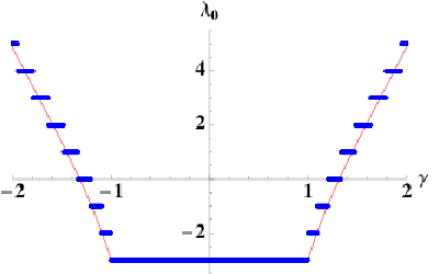
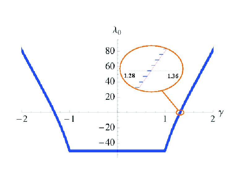
We observe that both $E_{0}$ and $\lambda_{0}$ depend strongly on the coupling strength $\gamma$. As this coupling is increased, the value of the (quantum) constant of motion at which the minimum energy is obtained remains constant until a threshold is reached, at which point it jumps to its next value. This same process repeats itself as $\gamma$ keeps increasing, $\lambda_{0}$ taking discrete values throughout (in contrast to its semiclassical counterpart, which is continuous), reflecting the quantum nature of the system. As $N$ increases, the width of the steps becomes smaller until the difference with the classical result seems negligible. However, the separation of $\lambda$-values always equals $1$ (cf. zoom in the figure). In the North Pole, the state is $|\nu\rangle\otimes|j,\,m\rangle=|0\rangle\otimes|j,\,-j\rangle$, so only one value of $\lambda_{0}$ (and of $E_{0}$) is had all through this region $-1<\gamma<1$, and it naturally coincides with the classical value. The same (dual) result is obtained in the South Pole.

This discrete behaviour in $\lambda_{0}$ is inherited in all the quantum observables of interest, as we shall see below. It is important to note the horizontal shape of the steps in $\lambda_{0}$ shown in Fig.(6). This is a consequence of the system being in resonance: $\Delta=0$. When the detuning parameter is taken away from resonance, the $\lambda_{0}$ steps acquire a slope given precisely by the difference in energy between the absorbed photons and the atom’s energy level separation.

Given the present possibility of confining a small number of atoms and performing non-demolition experiments on them, and the direct importance of these on cavity QED, quantum information theory, encryption, teleportation, and quantum optics in general, in all the results that follow, we take $N=6$ and $\Delta=0.2$ in order to illustrate the behaviour of a small system slightly away from resonance. The effect of the detuning parameter on the ground state energy, for $\Delta=\ -0.2,\,0,\,0.2$, is shown in Fig.(7). One notices that the width of the North Pole depends on the value of $\Delta$, as expected.

Fig(8) presents the expectation value of $\langle J_{z}\rangle/N$ for $N=6$ atoms and $\Delta=0.2$. The observable takes discrete values for the exact quantum solution while it is continuous for the semiclassical trial state. The inherited discreteness from $\lambda_{0}$, associated to quantum phase transitions as the structure of the ground state changes with $\gamma$, is evident. The semiclassical approximation follows the same trend.

For $\gamma^{2}<\omega_{A}$ all the atoms are concentrated in their lowest hyperfine level. It is natural to find that $\langle J_{z}\rangle/N$ takes on the value $-j/N$, which in the plotted case corresponds to $-0.5$, and the constant of motion takes its minimum value $\lambda=-3$. For values of $\gamma$ outside this region there are other occupancies. When $\gamma$ is very large the occupancy tends to zero, i.e., the two hyperfine levels are equally occupied. The dispersion $(\Delta J_{z})^{2}$ has values ten times smaller.

The expectation value $\langle\hat{n}\rangle/N$ of the photon number operator per number of atoms with respect to the ground state is shown in Fig.(9), for the exact and variational quantum results, for a system of $N=6$ atoms with a detuning $\Delta=0.2$. The fluctuation in the number of photons $(\Delta n)^{2}/N^{2}$ is also shown. Note that in the North Pole, $|\nu\rangle\otimes|j,\,m\rangle=|0\rangle\otimes|j,\,-j\rangle$, the number of photons is zero. Thus, the fluctuation must be zero and completely coincide with its semiclassical counterpart. Outside this region, the proposed trial function as a coherent state for the description of the electromagnetic field, which includes an infinite number of photons in its composition, greatly overestimates the quantum result: for $\gamma\approx 2$ there is approximately one photon per atom with very good agreement between the two procedures, while their corresponding fluctuations have at least a difference of a factor of six.

We have found that the ground state of the TC model does not present the phenomenon of squeezing in the matter components. However we propose to use the behaviour of the squeezing spin coefficient $\xi$ as an additional signature of the goodness of our trial state in reproducing the exact quantum solution. We can see in Fig.(10) that the squeezing coefficient exceeds the value of one for large values of the coupling parameter. This means that the trial state must have a very small overlap with the exact quantum state, and it is due to the multiple values of the constant of motion contained in the composition of our trial state.

The entanglement is usually regarded as a purely quantum correlation which plays an important role in quantum phase transitions [10, 11]. For the variational state the entanglement entropy between the matter and field is zero because it corresponds to a pure state (matter coherent state). It is then interesting to do a comparison with the entanglement between atoms in the semi-classical approach. Fig.(10) shows the entanglement entropy associated to the variational and exact quantum cases, for a reduced density matrix that eliminates the electromagnetic degrees of freedom and discriminates the matter part into the atoms occupying the lowest hyperfine level from the rest, and viceversa. Once again, the semiclassical result is a very good approximation to the exact one. The plots shown are for $N=6$ and $\Delta=0.2$. It is clear that for any $\lambda>-j$ (i.e., outside $\left|\gamma\right|\leq\sqrt{1-\Delta}$) there is entanglement between the atoms. In the thermodynamic limit $N\rightarrow\infty$, the behavior is the same with an even more abrupt slope at the separatrix. Besides, one can notice directly from this plot, that the entanglement entropy with $\gamma\approx 2$ is $S_{E}\approx 1.6$ nats; this compares favorably with a straightforward estimate of the maximum entanglement entropy available for a quantum system of $j=3$, which would yield $S_{E}=1.94$ nats.

An interesting measure, coming from quantum information theory, is the fidelity $F(\rho_{1},\,\rho_{2})$ [25], where $\rho_{i}$ denotes the density matrix of a system. This is a measure of how close two probability distributions are to each other, even for mixed states. In the case of two pure states, the measure is equivalent to the overlap. In our case, we want to compare the reduced probability distributions calculated from the exact model and from the variational model. Since they are both diagonal (cf. Eqs.(15, 27)), the expression for the fidelity is simple:

Fig.(11) shows the fidelity as a function of $\gamma$ both in resonance $\Delta=0$, and away from resonance $\Delta=0.2$, for the probability distributions mentioned above. At the North Pole (zero photons and all atoms in the ground state, $\lambda=-j$) the fidelity represents the overlap between the two states, and equals $1$. Each jump represents a value of $\lambda$ increased by $1$. The first and largest transition is found at the separatrix, while the other discontinuities occur at the quantum phase transitions. Note that $F$ diminishes at each of these for small values of $\lambda$ (small number of photons). In all these cases we have mixed states. After $\lambda=j$ (number of photons equal to the number of atoms) the dimension of the Hamiltonian matrix remains constant and $F$ increases at each transition (except for the anomalous case $N=1$). It is important to stress the fact that the fidelity is high and the probability distribution of the coherent state approximates very well the exact solution, especially for a small number of atoms and a large number of photons.

The composition of the ground state of the TC model can be analyzed both, in terms of the distribution of the atoms into the two hyperfine levels, and of the photon number content, be it for the exact energy ground state or for its variational approximation. Fig.(12) shows the composition of the trial and exact states for $N=6$, $\Delta=0.2$. The four plots show the change in the occupation probability as one crosses one arm of the separatrix: in this case, we move along $Path\ II$ in Fig.(1) and cross the separatrix at $\gamma=-\sqrt{0.8}$ from the Parallels region into the North Pole (recall that $\Delta=0.2$). The marked change due to the phase transition is obvious. While the composition of the ground state in both cases are very similar, one has to notice that the variational state is constituted by a distribution of $\lambda$’s in contrast to the exact quantum result which is described by only one $\lambda$-value. (This good approximation is a consequence of the fact that the distribution of $\lambda$’s is a gaussian centered at the quantum eigenvalue, as will be seen below in Fig.(14) and its corresponding discussion.) This quantum $\lambda$-value depends of the coupling parameter $\gamma$ considered in the TC Hamiltonian as can be seen in Fig.(6). It is important to stress that, for values of $\gamma$ far away from the separatrix ($\gamma=-1.5$ in the figure), the semiclassical occupation probability estimates very well the quantum result. The estimate is even better as $N$ increases, until they become almost indistinguishable, as shown in Fig.(13) calculated for $N=100$. However, as we get close to the separatrix ($\gamma=-\sqrt{0.8}$ for $N=6$; $\gamma=-1$ for $N=100$) the semiclassical approximation gets poorer. When we cross it, both distributions become a spike at $\lambda=m=-j$, and they remain so until the separatrix is crossed again. The distributions are exactly the same changing $\gamma$ for $-\gamma$ (cf. Fig.(13)).

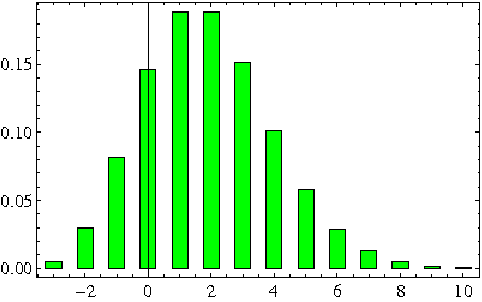
To calculate the distribution of the $\lambda$ values for the trial state one can use the coefficients (20). Fig.(14) shows the obtained distribution for $\gamma=-1.5$, $N=6$, and $\Delta=0.2$. Notice that there are approximately six different values of $\lambda$ with significative values in the probability distribution. The maximum is centered between $\lambda=1$ and $\lambda=2$; adjusting a gaussian distribution we get a mean $\mu=1.87$ and a standard deviation $\sigma=2.06$. For reference, the exact diagonalization gives $\lambda_{0}=2$ for this value of $\gamma$. While only values of $\lambda$ up to 10 were considered in this chart, these amount to 99.979% of the total contribution. This is the main reason why the tensorial product of coherent states constitutes a good approximation to the quantum ground state.

In order to explain the good approximation of the trial state in all the studied observables except for the fluctuations in the number of photons, one can study the way in which the number of photons is distributed in the ground state for each quantum eigenvalue $\lambda$. From our analysis on fidelity (cf. Fig.(11)), we expect the distributions for the variational state and the quantum state to agree inside the North Pole and away from the separatrix, but to show a strong disagreement at the separatrix itself. This is exactly what Fig.(15) shows, where, starting at the minimum value $\lambda=-10$, corresponding to $\gamma=\sqrt{1-\Delta}-0.01$ (just inside the North Pole), we increase $\lambda$ in steps of $1$, crossing the separatrix and reaching a value away from it at $\lambda=6$, corresponding to $\gamma=1.5$. We see that, even though the photon number distribution of the trial state is wider than the quantum case, the mean is the same. The top of Fig.(16), for $N=10,\ \Delta=0.2$ and $\gamma=5$ (corresponding to $\lambda=124$), shows this more clearly. Considering the contribution to the photon number probability distribution given by only the $\lambda$ value of the exact quantum solution, we obtain the narrow, darker bars in Figs.(15, 16). The amplitudes are necessary smaller since we have eliminated all contributions from other $\lambda$ values: for instance, with $N=10,\ \Delta=0.2$ and $\gamma=5$ the contribution of the values of $\nu$ to the state is of only $3.5\%$. However, a proper renormalization renders this distribution practically equal to that of the corresponding quantum photon number distribution, as illustrated in Fig.(16) (bottom).