One of the most exciting ideas of contemporary physics is to explain the origin of the observed structures in our universe as a result of quantum fluctuations in the early expanding universe. As first shown in the sixties [1], the amplification of quantum field fluctuations is an unavoidable consequence in a strongly time-dependent gravitational field [2, 3]. Fundamental physical implications were implemented some years latter to culminate, in the seventies, with the prediction of the evaporation of black holes with a black-body spectrum [4] and, in the eighties, when the inflationary model of the universe was introduced [5], predicting that small density perturbations are likely to be generated in the very early universe with a nearly scale-free spectrum [6]. In the nineties, the detection of temperature fluctuations in the cosmic microwave background (CMB) by the COBE satellite [7] appeared to be consistent with the inflationary cosmology predictions. In the present decade, the predictions of inflation have been confirmed in the specific pattern of anisotropies imprinted in the full sky map of the CMB, as reported, for instance, by the WMAP mission [8]. Moreover, an inflationary-type expansion also predicts the creation of primordial gravitational waves [9], whose effects still remain undetectable. Forthcoming experiments, such as the PLANCK satellite [10], may measure effects of relic gravitational waves and offer new trends for gravitational physics in the next decade. Therefore, it is particularly important to scrutinize the quantitative predictions of quantum field theory in an inflationary background. This is the aim of this essay.

As remarked above, a strongly time-dependent gravitational field necessarily amplifies vacuum fluctuations. This happens, typically, in a rapidly expanding universe and also in a gravitational collapse. The event horizon of a black hole acts as a magnifying glass that exponentially stretches very short wavelengths to macroscopic scales and generates a thermal flux of outgoing particles. Similarly, during exponential inflation, $ds^{2}=-dt^{2}+e^{2Ht}d\vec{x}^{2}$, a typical physical length, with comoving wavenumber $k$, increases exponentially $k^{-1}e^{Ht}$ and reaches the Hubble radius, $H^{-1}=$constant, at some time $t_{k}$ ($ke^{-Ht_{k}}=H$). These quantum fluctuations produce scale-free density perturbations and relic gravitational waves via a quantum-to-classical transition at the time of Hubble horizon exit $t_{k}$. The cosmic expansion farther stretches these scale-free primordial perturbations to astronomical scales.

Let us focus on the production of relic gravitational waves by considering fluctuating tensorial modes $h_{ij}(\vec{x},t)$ in an exponentially expanding, spatially flat universe: $g_{ij}=a^{2}(t)(\delta_{ij}+h_{ij})$, with $a(t)=e^{Ht}$. The perturbation field $h_{ij}$ can be decomposed into two polarization states described by a couple of massless scalar fields $h_{+,\times}(\vec{x},t)$, both obeying the wave equation $\ddot{h}+3H\dot{h}-a^{-2}\nabla^{2}h=0$ (see, for instance, [11]; we omit the subindex $+$ or $\times$). On scales smaller than the Hubble radius the spatial gradient term dominates the damping term and leads to the conventional flat-space oscillatory behavior of modes. However, on scales larger than the Hubble radius the damping term $3H\dot{h}$ dominates. If one considers plane wave modes of comoving wavevector $\vec{k}$ obeying the adiabatic condition [1, 2, 3] and de Sitter invariance one finds

These modes oscillate until the physical wave length reaches the Hubble horizon length. A few Hubble times after horizon exit the modes amplitude freezes out to the constant value $|h_{\vec{k}}|^{2}=\frac{GH^{2}}{\pi^{2}k^{3}}$. Because of the loss of phase information, the modes of the perturbations soon take on classical properties [12]. The freezing amplitude is usually codified through the quantity $\Delta_{h}^{2}(k)\equiv 4\pi k^{3}|h_{\vec{k}}|^{2}$. Taking into account the two polarizations, one easily gets the standard scale free tensorial power spectrum [11] $P_{t}(k)\equiv 4\Delta_{h}^{2}(k)=\frac{8}{M_{P}^{2}}\left(\frac{H}{2\pi}\right)^{2}$, where $M_{P}=1/\sqrt{8\pi G}$. It is easy to see that $\Delta_{h}^{2}(k)$ gives the formal contribution, per $d\ln k$, to the variance of the gravity wave fields $h_{+,\times}$

Due to the large $k$ behavior of the modes the above integral is divergent. It is a common view [11] to bypass this point by regarding $h(\vec{x},t)$ as a classical random field. One then introduces a window function $W(kR)$, multiplying at $\Delta^{2}_{h}(k)$ in the integral, to smooth out the field on a certain scale $R$ and to remove the Fourier modes with $k^{-1}<R$. One can also consider unimportant the value of $\langle h^{2}\rangle$ and regard the (finite) two-point function $\langle h(x_{1})h(x_{2})\rangle$, uniquely defined by $\Delta^{2}_{h}(k)$, as the basic object. However, $\langle h^{2}\rangle$ represents the variance of the Gaussian probability distribution associated to $h(\vec{x},t)$, which means that at any point $h(\vec{x},t)$ may fluctuate by the amount $\pm\sqrt{\langle h^{2}(\vec{x},t)\rangle}$ defining this way a classical perturbation. It is our view to regard the variance as the basic physical object and treat $h$ as a proper quantum field. Renormalization is then the natural solution to keep the variance finite and well-defined. Since the physically relevant quantity (power spectrum) is expressed in momentum space, the natural renormalization scheme to apply is the so-called adiabatic subtraction [13], as it renormalizes the theory in momentum space. Adiabatic renormalization [14, 2, 3] removes the divergences present in the formal expression (2) by subtracting counterterms mode by mode in the integral (2)

with $w_{k}=k/a(t)$. The subtraction of the first term $(16\pi Gk^{3}/4\pi^{2}a^{3}w_{k})$ cancels the typical flat space vacuum fluctuations. However, the additional terms, proportional to $\dot{a}^{2}$ and $\ddot{a}$ are necessary to properly perform the renormalization in an expanding universe.

For the idealized case of a strictly constant $H$, the subtractions exactly cancel out the vacuum amplitude [13], at any time during inflation, producing a vanishing result for the variance. Therefore, the physical tensorial power spectrum, the integrand of (3), is zero. Note that this surprising result does not contradict the fact that quantum fluctuations in de Sitter space produce a Hawking-type radiation with temperature $T_{H}=H/2\pi$ [15]. This temperature stems from the comparison of the modes (1) with those defining the vacuum of a static observer, located at the origin of coordinates, with metric $ds^{2}=-(1-H^{2}r^{2})d\tilde{t}^{2}+(1-H^{2}r^{2})^{-1}dr^{2}+r^{2}d\Omega^{2}$. The different time/phase behavior of both sets of modes (captured by non-vanishing Bogolubov coefficients) produces the Hawking temperature. However, their amplitudes are exactly the same [16].

Does it mean that inflation does not produce gravitational waves? No. For more realistic inflationary models, $H\equiv\sqrt{\frac{8\pi G}{3}V(\phi_{0})}$ slowly decreases as $\phi_{0}$ (the classical homogeneous part of the inflaton field) rolls down the potential towards a minimum. Tensorial perturbations are then expected, on dimensional grounds, to be produced with amplitude proportional to $\dot{H}$, instead of $H^{2}$. The form of the modes is now $h_{\vec{k}}(t,\vec{x})=(-16\pi G\tau\pi/4(2\pi)^{3}a^{2})^{1/2}$ $\times H^{(1)}_{\nu}(-k\tau)e^{i\vec{k}\vec{x}}$, were the index of the Bessel function is $\nu=\sqrt{9/4+3\epsilon}$ and $\epsilon$ is the slow-roll parameter $\epsilon\equiv-\dot{H}/H^{2}=(M^{2}_{P}/2)(V^{\prime}/V)^{2}$. The conformal time $\tau\equiv\int dt/a(t)$ is given here by $\tau=-(1+\epsilon)/aH$. The loss of phase information in the modes still occurs at a few Hubble times after horizon exit, converting the fluctuations to classical perturbations. Therefore, it is natural to evaluate the new integrand of (3) (i.e, the tensorial power spectrum) a few Hubble times after the time $t_{k}$. Since the results will not be far different from those at $t_{k}$, we use the time $t_{k}$ to characterize the results. The new tensorial power spectrum turns out to be then

where $\alpha\approx 0.904$ is a numerical coefficient. As expected, it is just the deviation from an exactly constant $H$, parameterized by $\epsilon$, which generates a non-zero tensorial power spectrum.

The above result would then imply that the tensor to scalar ratio $r=P_{t}(k)/P_{\cal R}(k)$ may be well below the standard predictions of single-field inflationary models. However, this is not necessarily the case since the scalar power spectrum $P_{\cal R}(k)$, which constitutes the seeds for structure formation, is also affected by renormalization. A detailed calculation, sketched in [17], leads to

where $\beta\approx 0.448$ is numerical coefficient and $\eta\equiv M_{P}^{2}(V^{\prime\prime}/V)$ is the second slow-roll parameter. Note that this contrasts with the standard prediction: $P_{\cal R}=\frac{1}{2M_{p}^{2}\epsilon(t_{k})}\left(\frac{H(t_{k})}{2\pi}\right)^{2}$ [11]. Since the scalar amplitude is also modulated by the slow-roll parameters the ratio $r$ is given by

which contrasts with the standard result $r=16\epsilon(t_{k})$. To translate this difference to a closer empirical level we have to introduce the scalar and tensorial spectral indices $n_{s}\equiv 1+d\ln P_{\cal R}/d\ln k,\ n_{t}\equiv d\ln P_{t}/d\ln k$, and the running tensorial index $n^{\prime}_{t}\equiv d{n_{t}}/d\ln{k}$. The standard expression for the relation between the tensor-to-scalar ratio $r\equiv P_{t}/P_{\cal{R}}$ and spectral indices (consistency condition) is: $r=-8n_{t}$. It is expected to be verified by any single-field slow-roll inflationary model, irrespective of the particular form of the potential. However, if we invoke renormalization we get a more involved consistency condition $r=r(n_{t},n_{s},n^{\prime}_{t})$. For illustrative purposes, in the simplest case of $n^{\prime}_{t}\approx 0$ and taking the approximation $\alpha\approx 2\beta$, the new consistency condition becomes

Note that this expression allows for a null tensorial tilt $n_{t}\approx 0$ while being compatible with a non-zero ratio $r\approx\frac{16}{5}(1-n_{s})$.

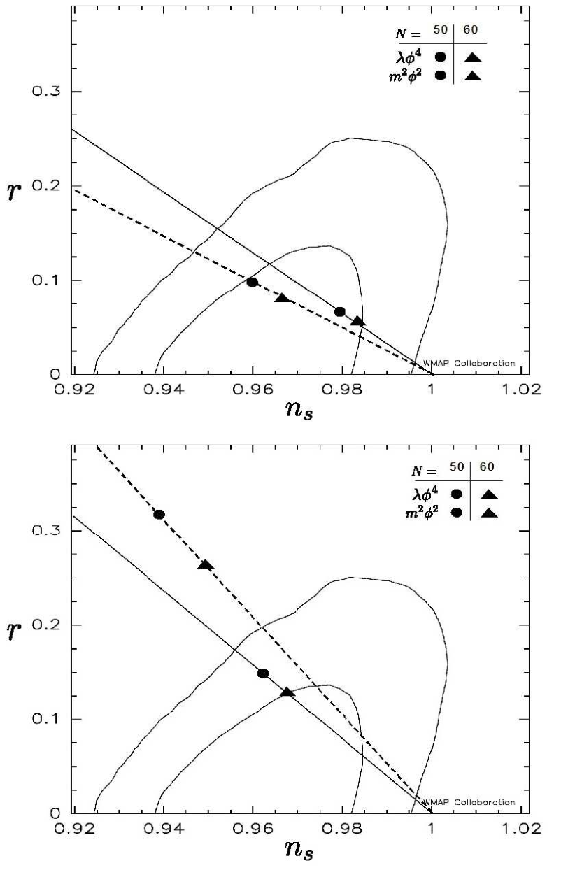
We can compare the new predictions with the standard ones on the basis of the five year WMAP results. We find [17], see Figure 1, that the new predictions agree with observation and improve the likelihood that the simplest potential energy functions (quadratic and quartic, respectively) are responsible for driving the early inflationary expansion of the universe. The influence of relic gravitational waves on the CMB will soon come within the range of planned satellite measurements, and this will be a definitive test of the new predictions.

References

- [1] Parker L., Phys.Rev.Lett. 21 562 (1968); Phys. Rev. 183, 1057(1969).
- [2] Parker L. and Toms D.J., Quantum field theory in curved spacetime: quantized fields and gravity, Cambridge University Press, (in press).
- [3] Birrel N.D. and Davies P.C.W., Quantum fields in curved space, Cambridge University Press, (1982).
- [4] Hawking S.W., Comm. Math. Phys. 43, 199 (1975). Parker L., Phys. Rev. D12, 1519 (1975). Wald R.M., Commun. Math. Phys. 82, 548 (1975).
- [5] Guth A., Phys. Rev. D23, 347 (1981). Starobinsky A.A., Phys. Lett. B91, 99 (1980). Linde, A.D., Phys. Lett. B108, 389 (1982); Phys. Lett. B129, 177 (1983). Albrecht A. and Steinhardt P. J., Phys. Rev. Lett. 48,1220 (1982). Sato, K., Mon. Not. Roy. Astron. Soc. 195, 467 (1981).
- [6] Mukhanov V.F. and Chibisov G.V., JETP Letters 33, 532(1981). Hawking, S. W., Phys. Lett. B115, 295 (1982). Guth A. and Pi, S.-Y., Phys. Rev. Lett. 49, 1110 (1982). Starobinsky, A. A., Phys. Lett. B117, 175 (1982). Bardeen, J.M., Steinhardt, P.J. and Turner, M.S., Phys. Rev.D28, 679 (1983).
- [7] Smoot, G., et al. Astrophys. J. Lett. 396, L1-L4 (1992).
- [8] Komatsu, E. et al, arXiv:0803.0547.
- [9] Grishchuk, L.P., Sov. Phys. JETP 40, 409 (1975); Starobinsky, A.A., JETP Lett. 30, 682 (1979).
- [10] Efstathiou G., Lawrence C. and Tauber J. (coordinators), ESA-SCI(2005)1.
- [11] Liddle A. R. and Lyth D.H., Cosmological inflation and large-scale structure, Cambridge University Press, (2000).
- [12] Kiefer C., Lohmar I., Polarski D. and Starobinsky A. A., Class. Quant. Grav. 24, 1699 (2007)
- [13] Parker L., hep-th/0702216
- [14] Parker L. and Fulling S.A., Phys. Rev. D 9 341 (1974).
- [15] Gibbons G. and Hawking S.W., Phys. Rev. D15, 2738 (1977).
- [16] Agulló I., Navarro-Salas J., Olmo G.J. and Parker L., Phys. Rev. Lett. 101, 171301 (2008).
- [17] Agulló I., Navarro-Salas J., Olmo G.J. and Parker L.,Phys. Rev. Lett. 103, 06131 (2009).