Factorization Structure of Gauge Theory Amplitudes and Application to
Hard
Scattering Processes at the LHC
Abstract
Previous work on electroweak radiative corrections to high energy scattering using soft-collinear effective theory (SCET) has been extended to include external transverse and longitudinal gauge bosons and Higgs bosons. This allows one to compute radiative corrections to all parton-level hard scattering amplitudes in the standard model to NLL order, including QCD and electroweak radiative corrections, mass effects, and Higgs exchange corrections, if the high-scale matching, which is suppressed by two orders in the log counting, and contains no large logs, is known. The factorization structure of the effective theory places strong constraints on the form of gauge theory amplitudes at high energy for massless and massive gauge theories, which are discussed in detail in the paper. The radiative corrections can be written as the sum of process-independent one-particle collinear functions, and a universal soft function. We give plots for the radiative corrections to , , , and , and to illustrate our results. The purely electroweak corrections are large, ranging from 12% at 500 GeV to 37% at 2 TeV for transverse pair production, and increasing rapidly with energy. The estimated theoretical uncertainty to the partonic (hard) cross-section in most cases is below one percent, smaller than uncertainties in the parton distribution functions (PDFs). We discuss the relation between SCET and other factorization methods, and derive the Magnea-Sterman equations for the Sudakov form factor using SCET, for massless and massive gauge theories, and for light and heavy external particles.
I Introduction
Soft collinear effective theory (SCET) [1, 2, 3, 4] is a field theory which describes the interactions of energetic particles which produce final states with small invariant mass. SCET was developed for QCD, but has recently been extended to spontaneously broken gauge theories with massive gauge bosons [5, 6, 7]. This allows one to compute electroweak corrections to Standard Model processes at high energies, and to sum electroweak Sudakov logarithms [6, 7]. One can compute QCD and electroweak corrections to parton-level scattering amplitudes with 1% precision. To achieve this accuracy, one needs to compute two-loop QCD and one-loop electroweak radiative corrections, and sum the large logarithms using renormalization group methods in SCET. An extensive analysis with plots of numerical results for parton processes such as dijet production, Drell-Yan, and top-quark production was given in Ref. [7]. The results included fermion mass effects (e.g. due to the top quark), mixing (which leads to ) as well as Higgs exchange corrections. The results are extended in this paper to include Higgs and gauge bosons. The purely electroweak corrections are substantial — 20% for pair production and 10% for production at 1 TeV rising to 50% and 25% respectively, at 4 TeV, and are much larger than two-loop QCD corrections.
The Sudakov double-logarithms arise as a result of soft and collinear singularities in radiation, and are a feature of exclusive amplitudes such as form-factors. They are absent in totally inclusive processes such as the total hadronic cross-section. There is some cancellation of the QCD Sudakov corrections in inclusive processes such as jet rates, because the infrared singularities cancel between real and virtual graphs. Jet cross-sections still have a residual double-logarithmic dependence on infrared parameters in the jet definition such as , and can have large radiative corrections. Unlike QCD, the electroweak Sudakov corrections do not cancel, even for a totally inclusive cross-section, because the initial state particles are not electroweak singlets [8, 9, 10].
Radiative corrections to high energy processes have been obtained previously using fixed order computations by many groups [8, 9, 10, 11, 12, 13, 14, 15, 16, 17, 18, 19, 20, 21, 22, 23, 24, 25, 26, 28, 27, 29]. The computations use infrared evolution equations [11], based on an analysis of the infrared structure of the perturbation theory amplitude and a factorization theorem for the Sudakov form factor [30]. We have checked our EFT results against these computations.
The computation of electroweak radiative corrections is greatly simplified by the use of effective field theory methods. The computation splits into a high-scale matching condition, and the EFT computation. The matching can be computed neglecting all low energy scales such as fermion masses, gauge boson masses, and spontaneous symmetry breaking. Secondly, the effective theory results depend only on the color structure of the amplitude, and are independent of the momentum structure. This is because the large momenta (i.e. the kinematic variables ) are labels in the effective theory, and not dynamical variables. Thus an amplitude in the effective theory can be treated as a number, with a different value depending on the kinematics. In contrast, in a computation without the use of effective theory methods, is a vertex in a Feynman graph, and the arguments of get integrated over in loop graphs. In gauge boson production, there are 10 possible kinematic structures [31], and they all evolve the same way in the effective theory.
In this paper, we explain in more detail the factorization structure of the high energy amplitudes which follows from the effective theory [32, 5, 6, 7], and extend our results to include external gauge bosons and Higgs scalars, so that we have the results for all standard model particles. The computations for longitudinally polarized gauge bosons use the Goldstone boson equivalence theorem [33, 34, 35, 36, 37, 38, 39, 40]. The factorization results hold both for the anomalous dimension, as well as for the low-energy matrix elements in the effective theory, i.e. for both the infinite and finite parts of the amplitude.
The factorization structure is rederived using the -regulator introduced in Ref. [41], because this gives the answer in a form which can be most easily compared with previous results using other methods [42, 43, 44, 45]. We show that the hard scattering amplitude can be written as a sum of process-independent one-particle collinear functions which depend on external particle energies, and a universal soft function which depends only on the external particle directions. The amplitude for a hard scattering process with external particles is given by combining the collinear functions for each external particle with the universal soft function. The collinear function for all standard model particles, and the universal soft function can be computed using the results given in this paper. The explicit expressions for the standard model are rather lengthy, because of the different possible fermion quantum numbers, and because of custodial violation which leads to mixing, , and to different radiative corrections for the and . For this reason, in this paper, we give the results for a broken gauge theory, with massless fermion doublets. The standard model results can be obtained straightforwardly from the results, and will be given explicitly in a companion paper [46]. All numerical plots shown here are in the full standard model, including Higgs corrections due to the top-quark Yukawa coupling.
The high energy behavior of scattering amplitudes for massive gauge theories is the same as that for massless gauge theories, since symmetry breaking is a soft effect and does not influence the high energy behavior of the amplitude. Thus our results are related to recent work on the infrared structure of gauge theory amplitudes [47, 48, 49, 45, 50, 51, 52], which we discuss in Sec. X. Of particular interest is whether the SCET amplitudes obey two properties, Casimir scaling and the sum-on-pairs form.
We compute the Sudakov form factor in a massive gauge theory, following the analysis of Magnea and Sterman [42]. This clarifies the connection between SCET results and the analysis using factorization methods. While SCET and factorization methods [53] use the same terminology of soft, collinear and hard amplitudes, the different contributions are not identical in the two approaches, even though their sum is the same. In our computation, the infrared sector of the gauge theory is under complete perturbative control, since the gauge bosons are massive, and the gauge theory is spontaneously broken. Thus we can compute the low-energy matrix elements, which are finite and free of infrared divergences. This provides additional insight into the structure of gauge theory amplitudes. In the usual QCD analysis, the low energy matrix elements are infrared divergent, and infinite in perturbation theory.
Using the results in this paper, one can compute radiative corrections in the effective theory to all partonic hard scattering processes, and thus to any hard scattering process at the LHC with an arbitrary number of external particles, if the high scale matching (step (2) below) is known. The high-scale matching is suppressed by two powers of a large logarithm relative to the EFT corrections. In the examples we have studied, the high scale matching (including QCD) is much smaller (by a factor of four or more) than the electroweak EFT corrections, so one can profitably use our EFT results even for cases where the high scale matching is not known. The only exception is the cross-section for , where the high-scale matching is almost 20%. The radiative corrections are also large for this case, and exceed 20% below 1 TeV.
The computation of the complete hadronic cross-section can be done using the following steps, shown schematically in Fig. 1:

(1) If the amplitude is the matrix element of a full theory operator, such as the Sudakov form factor for the scattering of a gluon by the operator , scale the operator using the standard model anomalous dimension to the scale (high-scale matching). If the amplitude is a scattering amplitude computed using vertices in the standard model Lagrangian, this step is not necessary, since the Lagrangian is independent.
(2) Compute the hard matching11 1 pun intended coefficient at a scale . This is a standard example of a matching computation to an effective field theory. is computed from graphs in the full theory, setting all small scales such as the gauge boson and fermion masses to zero. The resulting graphs are single-scale graphs, and have ultraviolet and infrared divergences, which are regulated using dimensional regularization, leading to terms. The ultraviolet divergences are cancelled by renormalization counterterms, and the infrared divergences are reproduced by corresponding infrared divergences in the effective theory. Thus is given by keeping the finite part of the full theory diagrams, and throwing away all singular terms in .22 2 The above procedure only works if dimensional regularization is used to regulate both the ultraviolet and infrared divergences. A check on the matching computation is that the infrared divergent terms must agree with the anomalous dimension in the effective theory. See, for example, Refs. [54, 55] for a more extensive discussion. The hard matching is independent of low scales such electroweak symmetry breaking and fermion masses, and so can be computed in the unbroken theory using gluons, and gauge bosons, without worrying about electroweak gauge boson mixing, even for processes such as production. All mass effects are included in the EFT computation in steps (4)–(6).
All scattering amplitudes are independent of the choice of . However, in perturbation theory, there is residual dependence from higher order terms that are not included in the computation. is chosen to be of order the hard scale in the scattering problem so that there are no parametrically large logarithms in , and all large logarithms are summed by renormalization group evolution. We will choose , the partonic center of mass energy in the collision.
The high-scale matching for processes involving a small number of external partons is known and is included in the examples considered in Ref. [7] and in this paper. The high scale matching, in general, does not obey the factorization structure of the effective theory amplitude. This is the only piece of the computation which cannot be computed using the effective theory results.
(3) Run the amplitude from the high scale to a low scale of order using the SCET anomalous dimension computed in . ( is SCET with dynamical gauge bosons). The SCET anomalous dimension is linear in to all orders [56], and the renormalization group evolution sums the Sudakov double-logarithms. For TeV, so the Sudakov corrections can be very large, and lead to a suppression of the cross-section. It is well-known that the QCD Sudakov corrections can have a huge effect on the cross-sections. The electroweak Sudakov corrections are also significant, ranging from 10%–50% depending on the process at energies of a few TeV, increasing rapidly with energy. The Sudakov double logarithms which are summed by the LL series are two powers of more important than the high-scale matching in step (1). The anomalous dimension is independent of the electroweak scale, and like the high-scale matching, can be computed in the unbroken theory.
(4) Compute the low-scale matching at by integrating out the , , Higgs and -quark, onto a theory containing only QCD and electromagnetism, which we call . The new feature found in Ref. [5, 6, 7] is that this low-scale matching in SCET contains a term of order . This term is related to the cusp anomalous dimension. No higher powers of a log appear to all orders in perturbation theory. For most processes, the low-scale matching correction is purely electroweak, since the gluon graphs are continuous through the electroweak threshold. The low-scale matching can be comparable to or slightly larger than the QCD contribution to the high scale matching because of the enhancement. There are low-scale QCD corrections for processes involving external -quarks, and here the corrections are much larger, of order 35%. The low-scale matching is one power of more important than the high-scale matching.
(5) Run the amplitude to (the factorization scale) using the anomalous dimension in . ( is SCET with dynamical gluons and photons). This gives the parton level scattering amplitude at the scale , i.e. the hard amplitude at , denoted by in Fig. 1.
(6) The last step depends on the experimental observable being computed. To compute a hadronic cross-section, one would first square the parton scattering amplitude and multiply by the partonic phase space to get the hard partonic cross-section . An SCET amplitude with two incoming collinear fields and outgoing collinear fields can be used to compute the cross-section for jets. This is an inclusive cross-section at the level of partons, i.e. each jet can contain any number of collinear partons, but it is exclusive at the level of jets, i.e. one only includes exactly jets, and no additional hard radiation. For such exclusive jet rates, one in general can have parton distribution functions (PDFs) describing the parton distributions inside the proton, as well as jet and soft functions [53]. These must all be scaled to the common scale , and then convoluted with the partonic cross-section , to get the experimentally measurable hadronic cross-section. The dependence of is cancelled by that in . This provides non-trivial constraints on the anomalous dimension, since the convolution running of , and must be cancelled by the multiplicative running of [57, 58]. For complete consistency, the parton distribution functions need to be extracted including QED corrections. The QED running below is very small, so one can simply drop this and match to PDFs obtained neglecting electromagnetic corrections.
The final step (6) above is common to all hadronic computations, and has been studied extensively. We have nothing new to say here. We therefore stop our computation at the end of (5). In the numerical results we present, we will choose .
Various software packages such as BlackHat [59], Rocket [60] and CutTools [61] are being developed to streamline the computation of QCD radiative corrections to experimentally relevant cross-sections at the LHC. These calculations typically include the QCD effects discussed in (1)–(4) above, but not the electroweak radiative corrections. They also perform the difficult task of taking partonic cross-sections and computing infrared safe observables (such as jet rates) in proton scattering. The electroweak corrections are independent of the QCD corrections to one-loop, and the mixed QCD-electroweak terms from renormalization group running at two-loops are tiny. One can then incorporate our results in the existing methods by using the results in this paper with as a multiplicative correction factor to the scattering amplitudes. If the partonic amplitude is needed at a scale , it can be obtained by using our results for and , and then scaling back up to using the pure QCD expressions.
The outline of the paper is as follows. In Sec. II, we give plots of a few representative processes to illustrate our results. We consider as an example of fermion scattering, for transverse electroweak gauge boson production, for longitudinal gauge boson production, for associated Higgs boson production, and . The kinematics and notation is given in Sec. III, and the structure of the logarithmic series in Sec. IV. Sec. VI discusses the EFT result that we need for our computations, which have been checked by explicit computation. There follows a long discussion in Sec. VII-Sec. XII on the general form of the radiative corrections to all orders in perturbation theory, which can be skipped by readers not interested in technical details. The topics discussed are only relevant beyond three loops, and away from the limit. Sec. VII discusses the -regulator, and Sec. VIII discusses the factorization structure of the amplitude. The general form of the scattering amplitude is given in Sec. IX. Casimir scaling, the sum-on-pairs form, and -factors are given in Sec. X. The decomposition into collinear and soft functions is given in Sec. XI, and the extension to heavy quarks in Sec. XII. The Goldstone boson equivalence theorem, and the one-loop radiative corrections, are summarized in Sec. XIII. Sec. XIV gives the results for the collinear and soft functions in an gauge theory. The Magnea-Sterman result for the Sudakov form factor is given in Sec. XV, and conclusions in Sec. XVI.
II Plots
The numerical results for a few representative standard model computations are shown here. The details of how these plots were computed will be discussed later in this article. All the computations have been done using QCD plus electroweak one-loop matching at and , and renormalization group evolution using the SCET QCD plus electroweak non-cusp anomalous dimension to two loops, and the QCD plus electroweak cusp anomalous dimension to three loops. The electroweak three-loop cusp anomalous dimension is only known neglecting the Higgs scalar contribution.
The results have a very small dependence on the Higgs mass. All the numerical results are for GeV. Changing to 500 GeV changes the rates by less than one part in .
The full standard model is matched onto at , and the electroweak gauge bosons, Higgs, and top quark are integrated out at . We will choose and in computing scattering rates. It is convenient to integrate out the electroweak gauge bosons, Higgs, and top quark at a common scale, so that one does not have to treat an effective theory with electroweak gauge bosons but broken gauge symmetry.
The dependence is very small in almost all the processes we have studied. Fig. 2 shows the variation in the cross-section as these scales are varied. is varied between and , and is varied between the two natural choices, and , which is approximately a factor of two variation. A similar plot of the variation for is shown in Fig. 3.


The only example with significant variation is transverse gauge boson production. Fig. 4 shows the variation for . The dependence is still very small, but the variation is nearly 10%. This is being investigated further. The high-scale matching is large for this process, almost 20%. We have checked that the dependence of the high-scale matching agrees with the EFT anomalous dimension.
The scale dependence is below 1% in all cases except production, so and will be held fixed in subsequent plots. The main contribution to the scale dependence is from the two-loop cusp anomalous dimension in the running, which is not cancelled by logarithms in the matching, since that has only been computed to one-loop. The scale-dependence would be even smaller if only the one-loop SCET anomalous dimension was used. The dependence increases with energy because of the term in the low-scale matching. The total radiative correction increases even faster.
The relative size of different contributions to the radiative corrections, such as the two and three-loop cusp and non-cusp anomalous dimensions, high-scale and low-scale matching, are shown for in Fig. 5, in Fig. 6, in Fig. 7 and in Fig. 8. We have determined the size of the electroweak corrections by turning them on and off in the effective theory, while keeping the full one-loop matching.


In processes such as , the tree-level matching has terms of order , from , and gluon exchange, and the one-loop matching has terms of order from box graphs. One has to decide whether to treat the tree-level matching as an electroweak correction to the term, and whether terms in the one-loop matching should be treated as electroweak corrections to the tree-level QCD matching, or QCD corrections to the tree-level electroweak matching. To avoid this, we have used the full one-loop matching in all comparisons. The EFT graphs are one-loop diagrams, so it is clear whether to call them QCD or electroweak corrections.
The electroweak radiative corrections are substantial, and increase rapidly with energy. For transverse production, the electroweak corrections exceed 20% at TeV. The corrections for transversely polarized gauge bosons are larger than those for longitudinally polarized gauge bosons and the Higgs. At high energies, longitudinally polarized gauge bosons and Higgs bosons behave like members of the scalar doublet, and their electroweak radiative corrections depend on the Casimir of the fundamental representation , whereas transverse gauge bosons depend on the Casimir of the adjoint , which is larger. The high-scale matching for transverse production is almost 20%, and both QCD and electroweak matching is important. The large dependence is an indication that the two-loop high-scale matching might be important for this problem.
The electroweak corrections are more important than the two-loop QCD cusp anomalous dimension.33 3 Note that at 1 TeV and at 5 TeV. The only corrections that are necessary for sub-1% accuracy are the one-loop QCD and electroweak corrections, the one-loop matching, and the two-loop QCD anomalous dimension. The two-loop electroweak and three-loop QCD corrections are completely negligible; even the two-loop QCD non-cusp anomalous dimension barely exceeds one percent in a few cases. The one-loop high scale matching can be as large as 10%. Higgs corrections proportional to the top-quark Yukawa coupling are a few percent. These arise even for processes not involving top quarks via virtual top quark loops in the anomalous dimensions for the longitudinal gauge bosons and Higgs (see Ref. [46]).


Finally, in Figs. 9–14, we show the complete radiative corrections to the scattering rate for some representative processes involving quarks, transverse and longitudinal gauge bosons, and the Higgs, normalized to the tree-level rate. At high energies, the radiative corrections suppress the scattering rate, but at lower energies, the radiative corrections lead to an enhancement. The rates are shown as a function of for different values of . The lower figure shows the total correction to the rate, whereas the upper panel shows only the electroweak contribution. The numerical values of the electroweak contribution are different from the previous plots, because they have been normalized to the tree-level rate. The previous plots computed the electroweak contribution using the ratio of the total rate including electroweak corrections, to the total rate without electroweak corrections.
Fig. 14 shows the radiative corrections to , which is a background for the Higgs search at the LHC. This process first occurs at one-loop in the standard model. We have not included the radiative corrections to the high scale matching , which would involve computing two-loop diagrams, but all the other radiative corrections have been included using the effective theory.
III Kinematics and Notation
We will compute amplitudes for an arbitrary scattering process with external legs in the high energy limit. The large energy scale will be denoted by , and can be chosen to be the center of mass energy in the collision. The effective theory computation is valid in the limit that the kinematic invariants are of order , and invariant masses are small, , , where is the mass of particle . The resulting amplitudes can be used, for example, to compute the rate for as long as the jet invariant masses are small compared with . The SCET computation neglects power corrections of the form and in the one-loop and higher radiative corrections, and these are estimated in Sec. V. The full dependence on mass ratios such as , which are order unity in the power counting, is included in the EFT computation.
It is convenient to introduce unit three-vectors , , which point along the direction of motion of the scattering particles. For incoming particles , define the null vectors and , with . For outgoing particles , and are defined by and .
In SCET, fast moving particles in the direction are referred to as -collinear particles, and are described by fields . A four-vector can be decomposed as
| (1) |
If is the momentum of an collinear particle, and , , then , , . If is chosen to point precisely along the direction of , so that , then and .
In an -leg scattering amplitude, all momenta are chosen to be incoming, so that for an outgoing particle , is the negative of the momentum of the particle. is still positive for outgoing particles, because of our definition of for outgoing particles.
A massive particle such as the top quark is described by a velocity four-vector , with , where , . For energetic top-quarks, it is sometimes convenient to use the four-vector , with in the high-energy limit. This allows for a smooth transition in the high energy limit to a massless description, with .
The Sudakov form factor will play an important role in this paper. The spacelike Sudakov form factor is defined as the particle scattering amplitude by an external current, with momentum transfer . It is convenient to compute the form factor in the Breit frame (see Fig. 15), where the particle is back-scattered, and the momentum transfer has .

The Sudakov form factor is an scattering amplitude, where the incoming and outgoing particle are identical. In the Breit frame, , so that and .
The labelling convention chosen for the Higgs doublet is
so that . The charged gauge and Goldstone bosons are
| (5) |
and the sign convention for the and photon fields is
| (6) |
The and fine structure constants are and respectively, and the QED fine structure constant is , with
| (7) |
We will use the abbreviations
| (8) |
A generic gauge coupling is denoted by , and the electromagnetic coupling constant is .
Anomalous dimensions, form-factors and matching coefficients will be expanded in powers of ,
| (9) |
IV Structure of the Logarithms
The schematic structure of the radiative corrections is
where the first row is the tree-level result, the second row gives the one-loop corrections, etc., and all the terms are added to give the total amplitude. The standard terminology used in the literature is to call the first row leading order, the second row NLO, the third row NNLO, etc. and refer to the term as LL, the term as NLL, etc. Thus the term is referred to as the NNLL term at NNLO.
In the leading-log regime, where , the terms have the form
and terms of high order become important.44 4 The leading double-log series exponentiates, and is convergent, i.e. has a series expansion with infinite radius of convergence. Clearly fixed order perturbation theory breaks down completely when get comparable to , and one needs to include all terms along and below the diagonal in Eq. (IV).
The SCET formalism gives a result for the logarithm of the amplitude in the form
which is the known form of the perturbation series for the Sudakov form factor [62, 63, 64]. Eq. (IV) implies many non-trivial relations between the coefficients in Eq. (IV). In the leading-log regime, the exponentiated series becomes
To get a reliable value for the amplitude in the leading-log regime, it is essential to sum the first two columns of Eq. (IV). In this case, the higher order terms are small and under perturbative control, even though the total radiative correction can be very large (order ). We will use the exponentiated form of the amplitude. The first column in Eqs. (IV,IV) is the LL series, the second column the NLL series, etc.
The SCET analysis automatically gives the amplitude in the exponentiated form Eq. (IV). By expanding the SCET result in a series in , one can recover the form Eq. (IV). The exponentiated form must be used for the QCD corrections. It also needs to be used for electroweak corrections in production at several TeV, where the electroweak corrections become order unity. At lower energies ( TeV) it is not necessary to sum the entire set of terms along and below the diagonal in Eq. (IV). It is still necessary to include the two-loop corrections, and in some cases, the three-loop terms. The SCET formalism automatically sums all these terms (as well as higher order enhanced terms). The two-loop terms can be obtained using a one-loop renormalization-group improved computation. We have checked that the SCET formalism reproduced the known two-loop , terms [11, 12, 13, 14, 15, 16, 17, 18, 19, 20, 21, 22, 23, 24, 25, 26, 27].
It is worth emphasizing that with the EFT theory method, no additional work needs to be done to sum the higher order terms. This is done automatically by the renormalization group. Instead one needs to work harder to drop these terms by expanding the SCET expressions in , and then truncating the series. By contrast, in a fixed order computation, one first computes the one- and two-loop graphs, matches the resulting amplitude to the infrared evolution equation and then exponentiates the resulting amplitude, so summing the higher order terms requires additional work.
V Estimate of Neglected Power Corrections
The EFT computation neglects power corrections in the one-loop and higher radiative corrections. There are also power corrections at tree-level, which arise from masses in the propagators and particle phase space. These are easy to include, and do not limit the computation. Thus the neglected power corrections are small, because they only arise from loop graphs.
To estimate the size of power corrections in the loop graphs, we compare the exact and EFT results for the one-loop Sudakov form factor with a massive gauge boson. The exact one-loop result is
| (34) | |||||
In the limit, this becomes
| (35) | |||||
which is the EFT result,
plus suppressed corrections. We define the power corrections as the difference . At ,
| (37) |
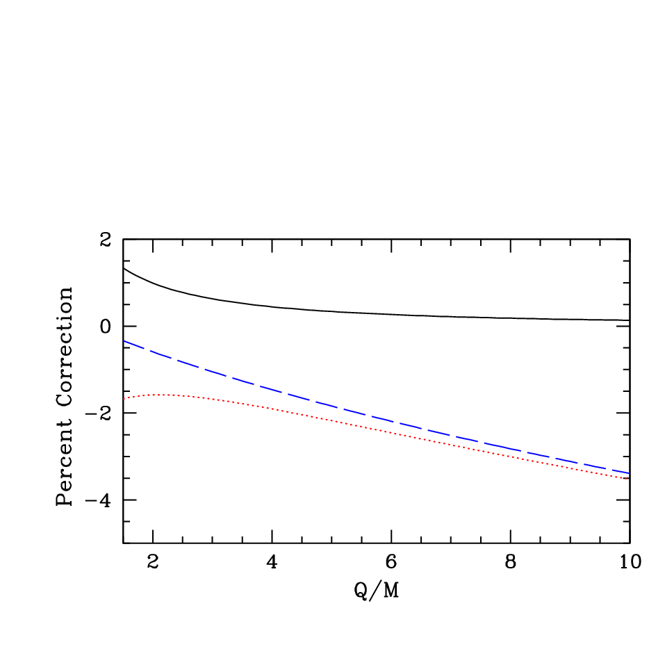
In Fig. 16, we have plotted the power corrections as a percentage of the tree-level value , using an gauge theory with coupling , the value of the standard model gauge coupling at . The power corrections shown by the solid black line are less than 2% even at , and fall below 1% by the time . The EFT radiative corrections, shown by the dotted red line, grow with energy.
The other place where power corrections enter is through the use of the Goldstone boson equivalence theorem to compute the cross-section for longitudinally polarized gauge bosons, since the polarization vector is replaced by the momentum . Here the power corrections exist even in the tree-level amplitude. In Fig. 17 is plotted the ratio of the

tree-level cross-section computed using the equivalence theorem, to the exact expression , as a function of the center-of-mass energy for different center-of-mass scattering angles . The ratio asymptotes to one, but the corrections do not go below 1% until . The correction is % for . Production threshold is .
The cross-section is suppressed by relative to the and cross-sections. The cross-section has been omitted in our analysis. In Fig. 18, we

plot the ratio of the to the cross-section. The rate falls with energy, and is sub-1% of the total cross-section at .
The parton-level results in this paper have an accuracy better than 1%, with the exception of production. From the estimates in this section, we see that they can be used for processes other than those involving external longitudinal and bosons at relatively low energies, times , while retaining their sub-1% accuracy. For processes, the use of the equivalence theorem introduces power corrections at tree-level, so the corrections are not sub-1% till much higher energies. One can achieve sub-1% accuracy at much lower energies by including the tree-level power corrections in the final result, and by including the tree-level rate for production. Then only suppressed power corrections are omitted, as for the Sudakov form factor, and the results can be used close to threshold with high accuracy.
VI The Effective Theory Amplitude
The next few sections contain a lengthy discussion of the general form of the scattering amplitude to all orders in perturbation theory. We have already seen that for practical purposes, a one-loop analysis augmented by the two-loop cusp anomalous dimension is sufficient. The general form of the amplitude to this order is known explicitly, and the subtleties discussed in the subsequent sections are not relevant. We therefore provide a brief summary of the subsequent sections, and the form of the amplitude.
A generic -particle scattering amplitude can have several different gauge invariant contributions. One writes the amplitudes and anomalous dimensions as matrices in a standard operator basis. For example, the amplitude can have the two possible color structures,55 5 The term color refers to the gauge quantum numbers, not just to QCD. written schematically as
| (38) |
where the color of the initial particles is combined to a color singlet, or color octet, respectively. The amplitude and anomalous dimensions are matrices in this operator basis. A more useful notation is to use operators in color space acting on the various particles [65], rather than matrices in a particular basis. is a color operator acting on particle . The action of the color operators on the particle fields is
| (39) |
where is the color matrix in the representation of particle . The minus sign in the first of Eq. (39) is because annihilates particle . One can think of as a field-theory operator acting by commutation, so that
| (40) |
Taking the hermitian conjugate then gives the second of Eq. (39). Then, for example,
| (41) | |||||
Thus is equivalent to the matrix structure
in the basis Eq. (38).
The number of color invariants grows rapidly with the number of external legs, and the color operator method provides a compact way of writing the group theoretic form of the amplitude. The soft anomalous dimension and matching has universal form when written using color operators.
VI.1 The Renormalization Group Improved Amplitude
At high energies, fixed order perturbation theory breaks down because of large logarithms of the form , which are of order in the log-counting, since all invariants () are of order . From the point of view of the high-energy theory, these logarithms arise from infrared divergences as . The same logarithms arise from ultraviolet divergences as in the EFT, and can be summed using the EFT renormalization group equations.
The renormalization group improved on-shell scattering amplitude (i.e. an -matrix element) has the schematic form [5, 6]
| (45) |
where boldface quantities are matrices, and denotes path ordering so that higher values of are to the right. The and scales are of order and , respectively, and the dependence cancels between the matching conditions and the renormalization evolution, so that is independent. The invariants are of order . denotes a possible dependence on kinematic variables that is explained below. Further details on the form Eq. (45) are given in Secs. VIII, X.
In Eq. (45), is the high scale matching coefficient at , and can be a function of all the invariants . It is independent of low-energy scales such as the gauge boson mass or fermion masses . The matching scale is chosen of order , so that are all of order unity in the log-counting.
The anomalous dimension is the SCET anomalous dimension used to evolve the operators from to . is given by the ultraviolet divergence structure of the effective theory, and is independent of low-energy scales such as and . The denotes linear dependence on and a possible dependence on cross-ratios (also referred to as conformal ratios) of the form
| (46) |
which are order unity in the log-counting, can potentially arise in scattering amplitudes with four or more external particles beyond two-loop order[47, 48, 49, 45, 50, 51, 52], and are discussed further in Sec. X.
In deep inelastic scattering and , the SCET anomalous dimension is linear in to all orders in perturbation theory [56, 66], and can be written as . is known as the cusp anomalous dimension, and will be referred to as the non-cusp anomalous dimension. The term is order in the log-counting, and is proportional to the unit matrix. The integral of this term is order , and gives the exponentiated Sudakov double-logarithms in high-energy scattering. The term is order unity in log-counting, and its integral gives an order contribution to . can have a non-trivial matrix structure in color space.
The analysis in Sec. VII–XI is concerned with determining the structure of the anomalous dimension and low-scale matching to all orders in perturbation theory, and determining what possible variables can occur in . For the applications discussed in Sec. II, it is sufficient to know the form of the anomalous dimension and matching to two-loop order. This is known by explicit computation, and many of the complications discussed in later sections do not occur to two-loop order. We summarize here the results to two-loop order. The reader not interested in the technical details of their derivation can skip directly from the end of this section to Sec. XIII.
The matching and anomalous dimension can both be written as the sum of collinear and soft contributions, and , where the collinear contributions are unit matrices in color space. The collinear running and matching can be written as the sum of one-particle contributions,
| (47) |
where the sum is over the incoming and outgoing external particles in the hard scattering process. The collinear contributions are process-independent, so that, for example, and for a quark have the same values in and in . The collinear anomalous dimensions have the form
Recall that is twice the energy of the particle. The first term is order in the power counting, and the second term is order unity. is the cusp anomalous dimension. At one-loop,
| (49) |
and the two-loop value is given by multiplying by the -factor, Eq. ().66 6 See Sec. X.4 for the definition and references. has no subscript because it does not depend on the particle.
The collinear-matching has the form
and at one-loop,
| (51) |
and does not depend on the particle. The collinear matching at the low scale has a dependence on the high scale through the term. is related to the cusp anomalous dimension, and is required for consistency of the low-scale matching, see Sec. XV.
The matrix dependence is in the soft anomalous dimension and matching. These have a universal form when written using the color operator notation,
where the sum is over all pairs of external particles in the scattering process. The two-loop values are given by multiplying by the -factor, as shown in Refs. [43, 44] for the soft anomalous dimension in QCD.
The soft-collinear split divides the amplitude into a collinear contribution which depends only on the energies of the individual particles and is independent of their directions, and a soft contribtion which depends only on the vectors and hence on the directions of the external particles, but not on their energies. The full amplitude depends only on the Lorentz invariant dot products , and the dependence on the vectors introduced by the effective theory cancels between the soft and collinear terms by reparametrization invariance [67, 68].
The anomalous dimension has a cusp contribution , which is order , and the rest, which will be referred to as the non-cusp anomalous dimension, given by and , collectively referred to as .
The low scale matching has proportional to the unit matrix which contributes at order , and with non-trivial matrix structure which contributes at order unity. is given by the term in the collinear matching, and by the terms in the collinear matching, and the soft matching . The low-scale matching does depend on the low-energy scales and . In the standard model, it depends on the electroweak symmetry breaking scale, and includes contributions from the top-quark mass and mixing. The new feature of the high-energy scattering problem first found in Refs. [5, 6, 7] is the presence of the single-log term in the low-scale matching. This term can be shown to exist by explicit computation, and is required by consistency of the effective theory — the dependence in the running from the cusp anomalous dimension , which is of order , is cancelled by the dependence of . One can prove that the low scale matching is order in the log-counting to all orders in perturbation theory, so that terms such as do not appear [5, 6, 7]. This is discussed further in Sec. VIII.
The leading-log (LL) series is given by the one-loop cusp anomalous dimension, the next-to-leading-log (NLL) series by the two-loop cusp anomalous dimension and the one-loop values of and , the NNLL series by the three-loop cusp, two-loop and , and one-loop and , and the NnLL series by the loop cusp, the -loop and , and the loop and .
Eq. (45) for the standard model sums the QCD and electroweak corrections, including cross terms such as , , or which depend on mixed products of the Yukawa, strong and electroweak coupling constants.
Table 1 shows the order that the various quantities are needed to sum the different series. The shows which terms have been included in our numerical results, and shows the terms which have been included except for the scalar contribution. The only quantities remaining to sum the NNLL series are the log term in the low-scale matching , and the scalar terms in the three-loop cusp and two-loop non-cusp anomalous dimension. The two-loop value of has been computed in Ref.[15] for fermions when , and is given in Eq. (282).
VI.2 The UV/IR Correspondence
The gauge theory under consideration is a spontaneously broken gauge theory with a Higgs in the fundamental representation, so that all the gauge bosons are massive. Our analysis is also valid in the more general case of an arbitrary broken gauge theory with massive gauge bosons. The advantage of studying this theory instead of a massless gauge theory such as QCD is that the infrared structure of the theory is under complete perturbative control, with the divergences being regulated by the gauge boson mass , if the gauge coupling at is weak.
The high energy behavior of a spontaneously broken theory is the same as that of the unbroken theory, since spontaneous symmetry breaking is soft, and can be neglected in the high energy limit. Thus our computations also gives the high energy behavior of gauge theory amplitudes in an arbitrary unbroken gauge theory with massless gauge bosons. The ultraviolet behavior of an unbroken gauge theory is identical to the infrared behavior in perturbation theory, so we also obtain information on the infrared structure of gauge theory amplitudes in perturbation theory, which is a topic of current interest [47, 48, 49, 45, 50, 51, 52].
In the broken gauge theory infrared divergences are regulated by the gauge boson mass, so the renormalized amplitudes are functions of , and , , and the scattering amplitudes are IR finite. In a massless gauge theory, the scattering amplitudes are infrared divergent, and can be regulated in perturbation theory using dimensional regularization, so they have the form with playing the role of . The form Eq. (45) holds for the massless gauge theory, with the low-scale matching replaced by a low-energy parton matrix element computed in perturbation theory. This is the same as Eq. (45) with in the terms:
| (54) |
where , and are unchanged from their values in the broken gauge theory. The terms in Eq. (54) are infrared divergences, and arise because one is computing on-shell scattering amplitudes with a fixed number of external particles. They cancel between real and virtual graphs if one computes experimentally measurable quantities such as jet production rates, which are infrared safe.
VII Factorization Regulator
In SCET, the collinear and soft integrals need an infrared regulator, which cancels in the total amplitude. A regulator is necessary for all factorization calculations — otherwise one can show that the term in the anomalous dimension, which leads to the Sudakov double logarithms, would be absent.
A convenient regulator is the -regulator introduced in Ref. [41]. The -regulator for particle is given by replacing the propagator denominators by
| (55) |
has mass dimension 2. This regulator can be implemented at the level of the Lagrangian, since it corresponds to a shift in the particle mass. The on-shell condition remains . The form Eq. (55) determines the regulator to be used for soft and collinear graphs in the effective theory.
In SCET, the -collinear propagator denominators have the replacement Eq. (55). Collinear gauge invariance requires a collinear Wilson line , so that collinear fields only appear in the combination . As shown in Ref. [41, 69], this is true even in the presence of the -regulator, since the collinear Wilson lines do not require a regulator after zero-bin subtraction [70, 71, 41, 69, 72].77 7 The necessity of subtractions has been shown previously using other regulators [73]. -collinear graphs only depend on the regulator , and are independent of for .
If particle interactions with a soft-gluon (), the interaction with a -regulator becomes
| (56) |
Using Eq. (1), and keeping only the leading term gives
| (57) |
where
| (58) |
It is convenient to use as the regulator for the soft gluon interactions, even though it is determined from by Eq. (58). has mass dimension 1.
The soft interaction Eq. (57) is invariant under the rescaling , , so that soft graphs can only depend on the combination . This can also be seen directly from
| (59) |
so that only the ratio appears in soft graphs.
We also need the -regulated form for graphs containing heavy particles to study processes such as top quark production. We will use the boosted HQET (bHQET) formalism of Refs [57, 58], in which heavy particles are described by HQET fields , where is the velocity four-vector and is a null vector along the direction of particle .88 8 We will use lower case subscripts for light particles and upper case subscripts for heavy particles. The momentum is , and is the boost. contains ultracollinear fields that couple to analogous to the collinear Wilson line for collinear fields . does not require a regulator after zero-bin subtraction [41].
For the propagator and vertex, Eq. (56,57) become
| (60) |
where
| (61) |
so that the HQET propagator is regulated by , and amplitude only depends on the ratio .
The soft interactions of the heavy quark are given in terms of a soft Wilson line , for which Eq. (56,57) become
where
| (63) |
and the amplitude only depends on the ratio . and for heavy quarks both have mass dimension 1.
In previous papers, we have used the analytic regulator [74, 75], defined by letting
| (64) |
where are dimensionless. The same regulator is also used in Feynman graph computations using the method of regions (see, e.g. Ref. [14]). The analytic regulator is scaleless, so that SCET soft-graphs vanish on-shell. However, the analytic regulator breaks the color Ward identities necessary to write the collinear fields in the form [32, 7] if there is more than one gauge invariant amplitude. It can used for the Sudakov form factor (where there is only one color invariant), while maintaining the form of the collinear fields.
VIII Factorization Structure of the Amplitude
The scattering amplitude computed in the effective theory is computed from soft and collinear diagrams. will refer to the amplitude, or to the anomalous dimension, depending on the context. We will use to denote the masses and any other quantum numbers of particle (such as whether it is a fermion or scalar), and to denote its gauge quantum numbers.The argument denotes dependence on the gauge quantum numbers of all the external particles, whereas denotes dependence on the gauge quantum numbers only of particle , etc. Note that all amplitudes depend on the total particle content of the gauge theory, for example through the -function and vacuum polarization diagrams. What and denote is dependence on the quantum numbers of the particular external particle(s) for a given scattering amplitude.
In the general -particle scattering amplitude, all the momenta and gauge indices will be treated as flowing into the vertex. Thus an outgoing particle with momentum in representation is treated as an incoming particle with momentum in representation . The analysis below holds for an operator at arbitrary momentum, so we do not assume that the total incoming momentum vanishes, e.g. for the Sudakov form factor (), momentum transfer is inserted at the vertex.
A generic -particle operator has the form
| (65) |
where are gauge labels, and is a Clebsch-Gordan coefficient to make a gauge singlet operator. Here is an -collinear external line which couples to -collinear gauge fields, but not to soft gauge fields. is the -collinear Wilson line in the representation of particle necessary for -collinear gauge invariance, and is a soft Wilson line in the direction in the representation of particle and contains soft gauge fields. The structure of the interaction is shown in Fig. 19, and shows how the gauge indices are contracted.

Soft gluons couple only to the s, the triple lines in Fig. 19, and they can interact with any of the triple lines, as shown in Fig. 20.

-collinear gluons can interact with and , so they interact with the double line and dashed line for a given direction . They do not communicate between two different directions.

The collinear interactions involve only the part of the operator. Thus they only depend on the interactions of particle , and are independent of all the other particles in the process. Note that the Wilson line is in the gauge representation of particle , and does not need a -regulator. Thus collinear gauge invariance implies that each collinear amplitude has the form (to all orders)
| (66) |
where is an abbreviation for all the quantum numbers of particle , such as its mass, and whether it is a fermion, scalar, or gauge boson. The amplitude is a unit matrix in gauge space since gets corrections which do not change the index . The index cannot mix with the other indices, since the other indices do not transform under -collinear gauge transformations. The exponential form is convenient for the subsequent analysis. The collinear amplitude depends on the regulator only for particle , which enters into the particle- collinear propagator.
The soft amplitude is given by graphs in which the gauge bosons couple to the soft Wilson lines via eikonal interactions. The soft amplitude can be written (to all orders) as
| (67) |
The amplitude is a matrix in gauge space, since the soft interactions can mix the gauge labels in Eq. (65), so is a matrix exponential. The amplitude is written as rather than for future convenience. depends on the gauge quantum numbers and directions of all the particles. The argument in Sec. VII shows that it only depends on and in the combination . Note that the soft graphs do not depend on the masses of the external particles, or whether they are fermions, scalars, or gauge bosons. Thus the amplitude does not depend on . The soft interactions do not generate , and so can only depend on the invariants .
The soft amplitude can depend on particle masses through vacuum polarization graphs such as those in Fig. 22. They arise from the mass-modes discussed in Ref. [57, 58]. This dependence is omitted from the argument of Eq. (67)

for simplicity, and does not change the following discussion. The dependence on particle masses is an invariant dependence, i.e. it does not depend on the particular external legs in the scattering amplitude.
It is well-known that the Sudakov form factor depends on , and that the -particle scattering amplitude depends on . This can be seen explicitly by a one-loop computation. If the soft and collinear sectors were truly independent, then the scattering amplitude would be completely independent of . This is because each collinear sector is Lorentz invariant and can only depend on one momentum at a time, whereas the soft sector does not depend on , so there is no way to generate . The flaw in the argument is that the collinear and soft sectors need a regulator to be separately defined, and communicate via the regulator. The dependence is generated through this regulator dependence. This is not specific to SCET, but is a universal feature present in any method which factors the total amplitude into soft and collinear contributions. All such factorization methods must necessarily introduce a factorization scale that acts as a regulator and enters both the soft and collinear functions. The dependence enters through this regulator dependence, as we will see explicitly below for the regulator.
The total amplitude is
| (68) |
and the matrix ordering between and is irrelevant since the collinear terms are proportional to . The amplitude is the product of the collinear and soft contributions since the different sectors are independent. The log of the scattering amplitude is
where matrix ordering between collinear and soft is again irrelevant because the collinear terms are proportional to .
The total amplitude is independent of the infrared regulator, since the SCET scattering amplitude in a massive gauge theory is not infrared divergent. This is because the effective theory has the same infrared behavior as the full theory, and the full theory has no infrared divergences since they are all regulated by the gauge boson mass. This implies that the regulator dependence must cancel between the soft and collinear terms.99 9 One can write down the integrals for the soft and collinear amplitudes, and first combine the integrands before evaluating the integral. This allows one to compute the total amplitude without the necessity of introducing a regulator such as the regulator [76, 77]. The only reason for the -regulator is that divergences are introduced in the effective theory by the split into collinear and soft sectors.
The cancellation of the regulator in Eq. () puts strong constraints on the form of the effective theory amplitude. The dependence must cancel between the soft function and the collinear functions. The collinear amplitudes are a sum of one-particle terms, each depending on a single , whereas the soft amplitude depends on the products of all possible pairs of s.
The soft function depends on variables . [Remember that .] It is convenient to rewrite these in terms of cross-ratios which are independent of and variables which depend on . Define
for and
| (71) |
for . In Eqs. (,71), the particles , and play a special role, and have been included explicitly in the indices of . Most of the time, we will keep these reference particles fixed, and denote the cross-ratios by . , so there are non-trivial independent cross-ratios. The cross-ratios Eq. () are homogeneous in and so have the same values if .
The cross-ratios are invariant under rescaling , and so one can make the replacement , i.e. , and write them in terms of ratios of dot products of momenta,
The cross-ratios first appear for , and so can enter into the scattering amplitude. They are absent for the Sudkaov form factor (). For two-particle scattering , the only cross-ratios are
in terms of the Mandelstam variables.
Define the remaining variables by
In terms of these variables
| (75) |
if we let if . Thus any cross-ratio of the which is invariant under rescalings of the can be written in terms of :
since cancel on substituting Eq. (75).
Then the variables can be written as a linear combination of and , so the soft function can be considered to be a function of and .1010 10 It is useful to use so that the variables are dimensionless. The collinear function is a function of (see Eq. (58)), so it can be regarded as a function of . The total amplitude can then be written as
| (77) |
where only the momentum and regulator dependence has been shown explicitly. Since is independent of , differentiating it w.r.t. gives
| (78) |
Since only depends on , differentiating w.r.t. gives
| (79) |
and all mixed partial derivatives of vanish. This implies that must have the form
| (80) |
a sum of matrix functions each depending on a single variable. Substituting Eq. (80) in Eq. (78) gives
| (81) |
from which it follows that both sides are a constant since and can be varied independently. The constant must be proportional to the unit matrix since the r.h.s. is. It can only depend on variables other than and which are common to both and and have been suppressed in Eq. (81). Thus one gets
| (82) |
so that only depends on the color of particle and the gauge boson mass, and is independent of particle masses, and whether they are scalars, fermions, or gauge bosons. Thus is a universal function independent of , since the color dependence is explicit through the argument .
Integrating Eq. (82) gives
and
| (84) | |||||
where . The dependence has cancelled, and the amplitude depends linearly on the combination . The final result Eq. (84) is completely symmetric under the exchange of particle labels. This is not manifest in Eq. (84) because the split of kinematic variables into and is not symmetric. The final expressions we need for our computation given in Sec. XIV are manifestly symmetric.
The form Eq. (84) is valid to all orders in perturbation theory. is related to the cusp anomalous dimension. The factorized form Eq. (84) is valid for the renormalized amplitude and for the anomalous dimension in the effective theory, both of which have the additive structure Eq. (77). The EFT anomalous dimension is given by the UV divergences in the EFT, and does not depend on IR scales such as and , so these variables can be dropped for . The anomalous dimension can depend on and on the directions , since these appear explicitly as labels on the EFT operator. The amplitude Eq. (84) is linear in to all orders in perturbation theory, a result first shown in SCET for deep-inelastic scattering in Ref. [56]. For the multiparticle case, the dependence is proportional to the unit matrix, and commutes with the other contributions.
VIII.1 The Light-Light Sudakov Form Factor
The above discussion works for four or more external legs, , where one can use the variables and defined by Eqs. (,). For , there are no cross-ratios, but one can still use Eq. () and Eq. (75), dropping in the final result Eq. (84).
For , the soft function depends only on the single variable , and there is only a single color invariant, so that there is no matrix structure. The derivation leading to Eq. (88) for the two-particle case has already been given earlier in several different ways [56, 5, 6, 7]. We repeat the derivation because we will use the results for (the Sudakov form factor) extensively in the remainder of this article. In Eq. (77), the soft function can be chosen to be a function of . Since is independent of , differentiating w.r.t. gives
| (85) |
Differentiating again w.r.t. gives
| (86) |
so that
Note that because the operator is a gauge singlet, and , so that there is only one independent color operator. We will drop the subscript on when we write the color dependence of the Sudakov amplitude.
Eq. (85) implies , so there is no subscript on . This also follows from the discussion below Eq. (81). The collinear function has the same value whether particle scatters via a two-particle operator, or via an -particle operator, so and are the same as in Eq. ().
Adding the pieces gives
| (88) | |||||
In deriving Eq. (88) we have used and
| (89) | |||||
where , since all momenta are incoming.
VIII.2 Change of Basis Transformation
The basis for cross-ratios Eq. () picked out particles , and . One can use a different reference set of particles for the cross-ratios, , and in Eq. (). The cross-ratios in the new basis are given in terms of the old basis by
| (90) |
The transformation is linear in , and does not involve , so linearity of Eq. (84) in is maintained, and changing the basis does not provide any additional constraints. If is linear in in one basis, then it remains linear in in any other basis. Linearity in is connected with Casimir scaling, and will be important in Sec. X.
IX The Scattering Amplitude
One can now write down the general expression for a hard scattering amplitude using the EFT method.
(1) One matches from the full theory on to SCET at a scale of order . This gives a column vector of coefficients of the allowed SCET operators. We will normalize so that it is dimensionless. is a column vector, and has the form
| (91) |
and can depend on the invariants which are order , and logarithmically on , but not on low scales parametrically smaller than , such as . Since is dimensionless, it can depend on ratios such as , which are invariant under an overall rescaling of the momenta, but are not invariant under individual rescalings . The invariance under is broken by the dependence, i.e. by the anomalous dimension of . is computed from the hard part of the diagram, i.e. by using pure dimensional regularization with all infrared scales set to zero. This is the usual procedure for computing a matching condition, and the EFT factorization methods do not apply to this part of the computation. is chosen to be of order to minimize the logarithms in .
(2) Run the coefficients from down to a low scale of order using the SCET anomalous dimension. The SCET anomalous dimension has the form Eq. (84), and can be written as
| (92) | |||||
are the analogs of , and for the anomalous dimension. Since does not depend on low scales such as or , these variables are dropped in Eq. (92). , and are obtained from the ultraviolet divergent terms in Eq. (84), and obey the factorization structure of the EFT amplitude. , which is the cusp anomalous dimension, was shown above to only depend on the color of particle , but not on whether it is a fermion, gauge boson, or scalar. Thus we have written it as where the color dependence is explicitly through the second argument. The function is then universal, i.e. there is no need to introduce different functions for each particle. While does not depend on the mass of particle , it can depend on whether the particle is a fermion or scalar or gauge boson, so we have included an argument (for statistics) in ; again there is no need for different functions .
For the Sudakov problem, the scattering of particle by an external current, , there is no color matrix structure, and
| (93) | |||||
using the results of Sec. VIII.1 and the form Eq. (88). for the Sudakov problem, which we require later, has been called , and the term has been absorbed into . The branch cuts are determined by analytically continuing the form factor from Euclidean to Minkowski space, or by an explicit graphical computation. While there is no color matrix structure, the anomalous dimensions till depend on the color of the particles (through ), which is why the dependence is retained in Eq. (93).
The evolution of the amplitude from is given by
| (94) |
where denotes -ordering with larger values of on the right.
(3) Compute the low-scale matching at . The matching is also constrained by the EFT form Eq. (84),
| (95) | |||||
is linear in (the terms) to all orders in perturbation theory. The existence of this logarithm in the low-scale matching, and linearity to all orders, was first pointed out in Ref. [5, 6]. and are square matrices. Previous studies of factorization have all been for massless gauge theories. Eq. (95) is the factorization form for the low-scale matching in a massive gauge theory, which has not been studied previously.
We break into the single-log term and the rest,
| (96) | |||||
so the low-scale matching can be written as
| (97) |
where the two terms commute.
For the Sudakov form-factor () for particle ,
| (98) | |||||
where for the Sudakov problem is denoted by , the term has been absorbed into , and there is no matrix structure.
The final result for the amplitude is (showing the scales at which the various pieces are computed)
| (99) |
and is independent of and . This is the amplitude given in Eq. (45).
It is worth emphasizing that the total amplitude in the gauge theory does not have the factorization properties studied here. The factorization properties only hold for the effective theory amplitude, and hence for and in Eq. (99) but not for the hard matching correction . Thus the factorization properties are obscured in an explicit diagrammatic computation. The effective theory reorganizes the computation to make the factorization structure manifest, analogous to the way in which heavy quark effective theory (HQET) makes heavy quark spin-flavor symmetry manifest [78].
IX.1 Consistency Conditions
independence of Eq. (99) gives
| (100) |
and independence gives
| (101) |
so
| (102) |
Comparing the terms on both sides gives
| (103) |
which relates the term in the low-scale matching to the cusp anomalous dimension. Thus the presence of the term in the low-scale matching follows from consistency of the effective theory [7].
X Casimir Scaling
The results of the previous section simplify dramatically at one-loop. The collinear graphs are proportional to the color factor and the soft graphs are a sum over pairs of two-particle terms proportional to . The collinear and soft amplitude can be written as
| (104) |
where is a sum over pairs of particles with . This is a special case of Eq. (), where the color dependence of the collinear and soft amplitudes has been explicitly written, so that and do not depend on color, and has no matrix structure. Furthermore, the function multiplying can only depend on the single variable , rather than all possible dot products, and so the EFT amplitude cannot depend on cross-ratios, which involve at least four particles.
The EFT anomalous dimension and matching Eqs. (128,129,130,131) simplify considerably because of the restricted form Eq. (104). It is simplest to rederive the anomalous dimensions and matching conditions which follow from the -cancellation conditions starting from Eq. (104), rather than imposing the restriction of Eq. (104) on the results of the previous section. The answer is
and the derivation is given in Appendix C. The functions on the r.h.s. no longer depend on the color quantum numbers, and the matrix function has been replaced by a single function .
X.1 Anomalous Dimension
Assuming Casimir scaling, Eq. (104), the anomalous dimension Eq. (92) simplifies to
| (106) | |||||
and the Sudakov anomalous dimension Eq. (93) becomes
| (107) | |||||
using .
It is convenient to break the anomalous dimension into a collinear and soft anomalous dimension, the precise definition of which is given in Sec. XI for the general case. The collinear anomalous dimension is
| (108) | |||||
the soft anomalous dimension is
and the total anomalous dimension is . The soft anomalous dimension for an -leg amplitude has a universal form, and is completely determined in terms of the cusp anomalous dimension. At one-loop,
| (110) |
Eq. () is also valid at two-loops.
X.2 Low-Scale Matching
Assuming Eq. (104), the low scale matching Eq. (95) simplifies to
| (111) | |||||
is linear in (the terms) and in to all orders in perturbation theory.
We break into the single-log term and the rest, so Eq. (96) becomes
| (112) | |||||
so the low-scale matching can be written as
| (113) |
where the two terms commute.
For the Sudakov problem
| (114) | |||||
The matching can also be written as the sum of a collinear contribution
| (115) | |||||
and a soft contribution
with . The soft matching for an -leg amplitude has a universal form, and is completely determined in terms of the single-log term in the matching, which is related to the cusp anomalous dimension. At one-loop,
| (117) |
The above expressions give a remarkable simplification in computing scattering amplitudes. The collinear contributions are a sum over one-particle terms which do not depend on the scattering process, and the soft contributions are universal. The soft functions have the minimal form necessary to restore reparametrization invariance [67, 68] (i.e. boost invariance) of the EFT amplitudes. For back-to-back particles , and .
X.3 Form of the EFT Functions
Comparing the formulæ in this section with Eqs. (92,93,96,114), we see that
| (118) |
so that the color dependence is factored out into a prefactor. In addition, the non-trivial matrix structures and in the soft contribution are determined in terms of scalar functions and which appear in the Sudakov problem.
X.4 Higher Order
The one-loop functions Eq. (118) and the anomalous dimension Eq. (107) and amplitude Eq. (111) have two very special properties. The first is proportionality to , which is referred to as Casimir scaling. Obviously, this is a trivial result at one-loop, since the one-loop graphs all explicitly have this form, but it is non-trivial at higher orders. The cusp anomalous dimension has been computed to three-loop order [79], and obeys Casimir scaling to this order. The cusp anomalous dimension is
| (119) |
where the -factors are
Casimir scaling can be seen from the proportionality of to , so that all three terms in are proportional to .

It appears that the term in violates Casimir scaling; however, it originates from the two-loop vacuum polarization correction Fig. 23, and is from , and so the same for all particles, and does not depend on the particular particle whose cusp anomalous dimension is being computed.
The non-cusp part of the collinear anomalous dimension does not obey Casimir scaling. The one and two-loop terms for fermions are [14, 15]
and the term in violates Casimir scaling already at two loops. In color operator notation, it is proportional to . The three-loop value is known for a gauge theory with only fermionic matter [79].
The cusp anomalous dimension is the anomalous dimension of a Wilson loop with a point where the tangent vector is discontinuous (the cusp) [80]. Casimir scaling of Wilson line expectation values has been studied extensively in the literature, and there has been recent interest in this question [43, 44, 47, 48, 49, 45, 50, 51, 52]. Casimir scaling of Wilson loops has also been studied on the lattice, to test whether the string tension is proportional to the color Casimir of the quark. Recent results seem to indicate there is deviation from Casimir scaling [81] for the string tension. Casimir scaling of Wilson loops does not hold when non-perturbative effects are included. For example, large Wilson loops in the fundamental representation are confining and have an area law (in the absence of light fermions), whereas those in the adjoint representation are screened, and have a perimeter law. In the large limit, one can relate the two, since screening is suppressed [82, 83].
The collinear anomalous dimension respects Casimir scaling at least till three loop order, by explicit computation [79]. Recently, Aybat et al. [43, 44] have shown that the soft anomalous dimension matrix at two-loop order also respects Casimir scaling, i.e.
| (122) |
where is the same factor as for the collinear anomalous dimension, and is a number. Thus the entire two-loop anomalous dimension matrix can be obtained by multiplying the one-loop matrix by , as can the term in the two-loop matching.
For practical LHC computations, we only need the one-loop electroweak corrections, the one-loop QCD matching, and the two-loop QCD running. The one-loop terms have the nice and sum-on-pairs form. The results of Aybat et al. [43, 44] tell us that this form can also be used for the two-loop anomalous dimension. The two-loop non-cusp collinear anomalous dimension does not obey Casimir scaling, but it is a one-particle term and can also be trivially included in the results.
An interesting question currently being investigated is whether Casimir scaling continues to hold at higher orders. Becher and Neubert [51] have shown that the soft anomalous dimension should continue to have the form at three-loops, and have suggested that this form persists to all orders. If this form holds at higher orders, then the form derived in Sec. XI in terms of collinear and universal soft functions will continue to hold at higher order. For the electroweak problem, we need not only the anomalous dimension, but also the low-scale matching , and it would be interesting to investigate the form of at higher orders. The Becher-Neubert [51] argument that there are no color structures at two and three-loops other than implies that the low-scale matching should continue to have this form to three-loops.
X.5 Sum on Pairs
The results in Secs. X.1,X.2 have two properties — they are proportional to , and they are linear in , or equivalently in . Linearity in implies that the amplitude can only depend linearly on the cross-ratios ; higher powers would induce terms. The entire EFT one-loop result, including the low-scale matching, has linearity in both and in . The color structure follows trivially from the color factors of a one-loop graph, and linearity in can be seen by explicit computation. As shown in Ref. [7], an amplitude of this form can also be written as a sum-on-pairs over two-particle Sudakov form factors weighted with ,
| (123) |
Thus all the information in the scattering amplitude is contained in the Sudakov form factor.
Becher and Neubert [51] give a proposed form for the all orders anomalous dimension, which is both linear in and in , so that the sum-on-pairs formula Eq. (123) would hold to all orders. Ref. [7] used the analytic regulator for SCET. On-shell soft graphs vanish with the analytic regulator, so the entire amplitude arises from collinear graphs. The analytic regulator has the big disadvantage that the -collinear sector fields cannot be combined into the form of a single Wilson-line; instead one has separate -collinear Wilson lines for each particle not in the -direction, and the different collinear sectors have interlocking color structures [41]. This complication does not hold for amplitudes with a single color structure, such as the Sudakov form factor, or particular scattering processes such as in QCD (quix production). There is also effectively only a single color structure in the large- limit, because color reordering of the operators is suppressed by . The mixing is only suppressed for a suitable basis of operators, those written using products of color matrices in cyclic order.1111 11 In the double-line notation [84], each color connected part of the operator should consist of quark lines with alternating directions for the arrows, which are color-paired as one moves around the vertex in cyclic order, so that one has a planar vertex [85, 83]. Thus in the example considered in Ref. [86], one should use the basis , and rather than , and for the operator basis. One can then see that the anomalous dimension matrix in Ref. [86] becomes diagonal in the large- limit. In Ref. [7], it was shown that for amplitudes with a single color structure, linearity in holds to all orders. Thus a check of the Becher-Neubert proposal requires a four-loop computation away from the limit.
Linearity in implies that the amplitude and anomalous dimension have the form
| (124) | |||||
where
| (125) |
and do not depend on the cross-ratios. Imposing in addition linearity in for the terms and in for the rest reduces the amplitude back to Eq. (115). Only using linearity in gives the general form Eq. (84) with a restriction on the color structure of the terms, but no constraint on the dependence on cross-ratios.
XI Collinear and Soft Functions
The factorization form Eq. (84) of the EFT scattering amplitude allows us to efficiently compute the radiative corrections to high energy scattering processes, such as those needed for the LHC. The factorization structure studied in Sec. VIII provides a more compact way of writing our previous EFT results, by dividing the EFT scattering amplitude into a sum of one-particle collinear contributions, and a universal soft function. The procedure we follow is that used by Aybat, Dixon and Sterman [44] to separate the amplitude into jet and soft functions. We will use the name collinear function, rather than jet function, since the term jet function has already been used in the SCET literature for a different quantity. This decomposition will be used both for the anomalous dimension and for the low-scale matching .
The SCET computation automatically breaks the amplitude into a product of collinear and soft contributions. The splitting, however, is regulator dependent, and each piece depends, for example, on if one uses the -regulator. This is a generic feature of any factorization procedure which cannot be avoided, because the term in the SCET anomalous dimension is generated precisely by this regulator dependence. It is nicer to reorganize the amplitude into regulator-independent terms which have the same factorization properties as the SCET collinear and soft contributions. The basic idea is to write the effective theory amplitude as the product of the square-roots of the Sudakov form factor in SCET for each external particle, and the rest. The square-root of the Sudakov form factor in the effective theory (i.e. the form factor without the high-scale matching) is called the collinear contribution, and the rest is the soft contribution. Since the total amplitude and the SCET Sudakov form factor are both regulator-independent, this provides a regulator independent split of the amplitude into collinear and soft parts, which, as we will see, respects the factorization structure of Eq. (84). Our definition of the collinear function is identical to that of Aybat et al. [44] for the jet function. Aybat et al. define the soft function in terms of a ratio of web functions regulated by taking the directions away from the null direction, and then taking the light-like limit. We have used a different regulator and defined the soft function in terms of SCET amplitudes, but the final result is the same.
The Sudakov form factor for particle is the amplitude for , where both particles are of type , and in the Breit frame.1212 12 i.e. the Sudakov form factor is evaluated at the same energy that particle has in the -particle scattering process. An alternate choice is to evaluate all the functions at some common momentum transfer, such as . The collinear anomalous dimension is defined as one-half the anomalous dimension for the amplitude, Eq. (92), and can be written using Eq. (93) as
| (126) | |||||
Half the log of the Sudakov low-scale matching gives the log of the collinear matching
| (127) | |||||
using Eq. (114).
Now consider an arbitrary hard scattering process with external lines, where the particles have energies . We will define the collinear anomalous dimension and collinear low-scale matching by summing Eq. (126) and Eq. (127) evaluated at , and summed over all external lines. They are proportional to the unit matrix in color space. The total collinear anomalous dimension is the sum of one-particle terms
| (128) | |||||
as is the collinear low-scale matching
| (129) | |||||
The soft anomalous dimension is defined as the difference of the total anomalous dimension and collinear anomalous dimension. Using Eq. (92), we find
| (130) | |||||
The log of the soft matching is the difference of the logs of the total matching and the collinear matching ,
| (131) | |||||
and the total anomalous dimension and log of the low-scale matching are
| (132) |
The decomposition of the anomalous dimension and matching into soft and collinear functions discussed above is that used by Aybat et al. [44]. The soft/collinear split is related to the decomposition of the SCET amplitude into soft and collinear graphs, but is not identical. The basic difference is that in an -leg process, the soft contribution of the Sudakov form factors for each external particle has been added to the collinear function and subtracted from the soft functions (the and terms in Eq. (128,129,130, 131)). This cancels the regulator dependence of the SCET collinear and soft functions, and provides a regulator-independent definition for the two functions.
The collinear functions are process-independent, and can be computed directly from the Sudakov form factor. The cusp part of and of are of order in log-counting, whereas the remaining terms of , , as well as , are order unity. One can move the terms from the collinear factors into the soft factors by rewriting . It is more convenient to leave the order terms in the collinear functions, where they are explicitly proportional to the unit matrix. In addition, the form for the soft function remains valid for heavy quarks, so that the same soft function can be used for SCET and HQET fields.
Assuming the Casimir scaling form Eq. (104) allows and to be written in a much simpler form. Using the general form given in Sec. X for the anomalous dimension and amplitude, the collinear and soft anomalous dimensions and matching reduce to Eqs. (,,115,110) given in Sec. X. This is the form we need for the NLL standard model computations, which use one-loop matching and two-loop running, for which Casimir scaling is known to hold.
XII Heavy Quarks
We can also compute the scattering amplitude for external legs, where legs are light, and treated using SCET fields , and legs are heavy and treated using boosted HQET fields (bHQET) , [57, 58]. The SCET operators are given by Fig. 24, where, for a heavy quark, the external dashed line is replaced by a HQET field.

The collinear graphs have the same form as before, Eq. (66). The on-shell HQET graphs are also a sum over the external heavy particles,
| (133) |
The HQET graph does not depend on the heavy particle mass, since it does not enter the HQET computation. The soft amplitude is given by graphs in which the gauge bosons couple to the soft Wilson lines and via eikonal interactions. The soft amplitude can be written (to all orders) as
| (134) |
The two amplitudes only depend on the combinations , and as shown in Sec. VII.
The log of the scattering amplitude is
| (135) | |||||
where matrix ordering is again irrelevant because the collinear and HQET terms are proportional to , and we have written the and dependence in terms of Lorentz invariant dot products.
By a now familiar argument, the cancellation of the regulator in Eq. (135) puts constraints on the form of the effective theory amplitude. Since the form Eq. (135) is identical to Eq. () when there are no massive particles, the results of Sec. VIII hold. The only difference is that for heavy quarks, the collinear functions are replaced by HQET functions
analogous to Eq. (), where . does not depend on , since is not a parameter in bHQET. is not the same function as for a massless quark, but is. Eq. (84) becomes
| (137) | |||||
where because the relation between and is now Eq. (63). The soft function depends on color factors or cross-ratios involving all the particles, and any three particles (heavy or light) can be chosen as the reference indices in defining and .
Equation (137) is the general form for the SCET amplitude and anomalous dimension, and can be used for processes involving any combination of heavy and light particles.The change on replacing a light quark by a heavy quark is and in the collinear function. Thus the results of Secs. X and XI can also be used for heavy quarks with this substitution.
XII.1 Matching from SCET to bHQET
In processes where , the external particle is treated as an SCET field for , and as a bHQET field for , and we need to compute the matching correction at the scale between the two theories. This result is need, for example, to compute QCD corrections to production.
The difference between graphs in the theory above and below is in the treatment of -collinear interactions involving the heavy particle. In the theory above , they are given by , and in the theory below , by . In the amplitude Eq. (135), the difference is that is replaced by the corresponding for each external heavy particle. Thus for each particle making the transition from SCET to bHQET, the matching factor is
| (138) | |||||
The computation in the theory above is done on-shell with , and since one can set to compute the matching. The -regulator is not needed, and dimensional regularization is sufficient to regulate the infrared divergences. The difference is infrared finite.
The matching only depends on the collinear functions for light and heavy particles. The soft function remains unchanged at the SCET bHQET transition. The one-loop matching conditions are given in Table 2,
XII.2 The Heavy-Light Sudakov Form Factor
The heavy-light Sudakov form factor is the scattering of an incoming HQET field (particle 1) to an outgoing collinear field (particle 2) by an external current, similar to the decay process studied in Ref. [1]. The result is given using Eq. (137) for the case . The anomalous dimension is
| (140) | |||||
where also encode whether the particle is heavy, and we have dropped the subscript on since . Note that all heavy particles are the same, i.e. it does not matter if they are fermions, scalar, or gauge bosons. The low-scale matching is
| (141) | |||||
XII.3 The Heavy-Heavy Sudakov Form Factor
The Sudakov form factor for two heavy external lines is
| (142) | |||||
and the low-scale matrix element is
| (143) | |||||
The heavy-light anomalous dimension and matching are the average of the heavy-heavy and light-light values.
XII.4 Form Factor Relations
From the results in Secs. XII.2, XII.3, we see that
| (144) |
where and are light and heavy particles, and have the same color. This relation is satisfied by the EFT form factors. It is also satisfied by the full form factors in the limit , and
| (145) |
because the high scale matching condition is independent of particle masses, and cancels out, as does the matching between SCET and HQET for each external heavy line. Eq. (145) holds regardless of whether , and are widely separated, , or and are comparable. So it also holds for the massless gauge theory with the infrared divergences cancelling in the ratio.
XIII The Equivalence Theorem
The radiative corrections at high energy for longitudinally polarized massive gauge bosons can be most easily computed using the Goldstone boson equivalence theorem [33, 34, 35, 36, 37, 38, 39, 40], which relates the gauge boson amplitude to that of the corresponding (eaten) Goldstone boson,
| (146) | |||||
up to corrections which vanish in the high energy limit. The l.h.s. is the -matrix for an initial state to scatter to a final state, and the r.h.s. is the corresponding amplitude (made more precise later) with the gauge bosons replaced by the corresponding (unphysical) Goldstone boson. is a radiative correction factor which is one at tree-level, and are the energies of the gauge bosons. The existence of was first pointed out by Bagger and Schmidt [38]. The equivalence theorem only holds for the -matrix for physical states. All longitudinal gauge bosons must be simultaneously replaced by the corresponding for the theorem to be valid. Thus and do not contain any longitudinal gauge bosons.
We briefly review the derivation of the equivalence theorem including the radiative correction , and then give the result for in the -scheme.
For a longitudinal gauge boson in the direction with energy , the momentum is with , and the longitudinal polarization is chosen to be , , , where is the physical mass of the gauge boson. In the high energy limit .
The general form of the two-point function in the Goldstone boson/longitudinal gauge boson sector is
where the projection operators are
| (150) |
The momentum flows into the blob through the line corresponding to the right index of the matrix (see Fig. 25).

At tree-level,
| (151) |
where and are the parameters in the gauge-fixing term, and in gauge at tree-level, and we have used the notation of Ref. [40]. The tree-level Goldstone boson mass is .
The BRST Ward identity implies1313 13 See Ref. [40] for an excellent discussion of BRST Ward Identities and the Equivalence Theorem.
| (152) |
where and are the truncated Green’s function for emission of a gauge boson and Goldstone boson with momentum . This gives the equivalence theorem factor
| (153) |
Gauge bosons with polarization in truncated Green’s functions are replaced by . Eq. (151) gives at tree-level.
The Ward identity Eq. (152) is exact. The scattering rates are given by the -matrix, which is given by multiplying the truncated Green’s function evaluated at by the wavefunction renormalization factor , and using the physical polarization . corrections are introduced by replacing the polarization by the momentum, , and then neglecting the term. The term can be computed using the Ward identity:
The r.h.s. is evaluated at the physical gauge boson mass even in gauge where the Goldstone bosons have mass . We will write Eq. () as
| (155) |
where is defined as though it is the wavefunction renormalization factor for ,
| (156) |
where the derivative is taken at a fixed (-independent) reference momentum. The quantity we need, the l.h.s. of Eq. (155) is independent of the choice of . is a fake -matrix element for , and defines the quantity on the r.h.s. of Eq. (146). It is computed like an -matrix element, but it is gauge dependent because it is not the scattering amplitude for a physical state.1414 14 This is true at one-loop even if so that the Goldstone boson and gauge boson masses are equal at tree-level. The gauge dependence cancels that in , so that the left-hand side is gauge independent. We have checked this by computing both quantities in gauge. The l.h.s. of Eq. (155) is also -independent. On the r.h.s. of Eq. (155), and the fake -matrix element are both -independent.
The results tabulated in Sec. XIV give the -matrix element for fermions and transverse gauge bosons. For longitudinal gauge bosons, we list the expression for the Goldstone boson , which is why we have included so that it behaves as much as possible like an -matrix element. The results in Table 3 are given in gauge, and is evaluated at the reference momentum , which is the tree-level gauge and Goldstone boson mass.
The one-loop results we will need are:
where . This expression, and the ones below can be analytically continued to using
| (158) |
The expression for in ’t Hooft-Feynman gauge in the scheme is
Notice the expression is independent as discussed earlier.
XIV Results
The results needed for a NLL analysis of hard scattering processes in the theory are summarized here. The computations for external (massless and massive) fermion and scalar states were already discussed in detail in Refs. [5, 6, 7]. They were presented previously using the sum-on-pairs form discussed in Sec. X.5. They are tabulated here using the collinear+soft function form discussed in Sec. XI. The new computations are those for external gauge bosons and Higgs bosons. The standard model results can be easily derived using the results presented here; however, the expressions are considerably more involved than those for the theory because custodial is no longer a symmetry. Thus one has to include the effects of mixing, , and the mass difference. For this reason, the standard model results needed to compute all standard model hard scattering processes are given in a companion paper [46].
The results for external transverse gauge bosons were computed by matching onto SCET operators where the gauge field is given by the SCET field,
| (160) |
The field does not produce longitudinal gauge bosons to leading order in the SCET power counting. The amplitude for longitudinal gauge bosons is computed using the Goldstone boson equivalence theorem discussed in Sec. XIII.
XIV.1 Collinear functions for the theory
The one-loop collinear functions are summarized in Table 3. The function is given in Appendix B of Ref. [7]. The row is for fermions, for scalars, for external transversely polarized gauge bosons, for the physical Higgs field, and for the unphysical Goldstone bosons, which are used to compute longitudinally polarized gauge bosons using the equivalence theorem. The upper section of the table gives the results for fermions, scalars and bHQET fields, including wavefunction renormalization, assuming that the only wavefunction graphs are gauge boson corrections to the propagator with the topology shown in the upper graph in Fig. 26.


The lower section of the table gives the results for fermions, scalars, bHQET fields, transverse gauge bosons, the Higgs, and unphysical Goldstone bosons, where the wavefunction contribution has been separated out explicitly. , etc. are the anomalous dimensions of the fields and is the finite wavefunction factor needed in the scheme, from the residue of the pole in the two-point Green’s function function, .
XIV.1.1 Running from to
The collinear anomalous dimensions are given using the column in Table 3.
For the fermions :
| (162) |
with .
The gauge field anomalous dimension at one-loop in gauge is
| (163) |
where is the coefficient of the first term in the -function,
| (164) |
so that the collinear factor for transverse gauge bosons is
(transverse ):
| (165) |
with and . The final expression is gauge invariant. There is a factor of the coupling constant in the high-scale matching for each gauge boson. The term in Eq. (165) converts that to . The term is absent in the expression for in Ref. [27].
The unphysical Goldstone bosons and Higgs are renormalized together as elements of the scalar doublet ,
:
| (166) |
with .
XIV.1.2 Matching at
The matching corrections at have to be computed in the broken electroweak theory, using Table 3. The collinear matching depends on the mass spectrum of the broken theory. The low-scale matching for the fermions is:

One can think of as a single collinear object which is matched in the effective theory onto the fields and (see Fig. 27). Custodial invariance implies that and get the same collinear matching. In the standard model, custodial is broken, and the corresponding expression reads
The collinear Wilson-line on the l.h.s. contains and fields, whereas on the r.h.s. contains only photon fields. The two functions in Eq. (XIV.1.2) are no longer equal. One also has different collinear functions for the left and right-handed quarks, top quarks, etc. For this reason, the complete standard model expressions are deferred to Ref. [46].
The collinear matching for the scalar doublet is:
where have the same collinear matching by custodial- invariance. There is an interesting subtlety in the scalar doublet matching for the standard model, which is discussed in Ref. [46].
The matching for the transverse gauge bosons is:
| (177) |
Again, custodial ensures that all have the same collinear matching, and we do not have to worry about mixing.
The functions are:
where
| (179) | |||||
XIV.2 Universal Soft Function
The universal soft functions is
| (180) |
in terms of which, the soft anomalous dimension and low-scale matching are
| (181) |
For the Sudakov problem, there are only two particles, and , so that , and the soft contribution vanishes. The Sudakov computation is thus entirely given by the sum of the collinear functions for the two external legs.
The soft function has a universal form when written in the operator form Eq. (181). For numerical computations, it is more convenient to choose a basis of gauge invariant operators, and write the soft-anomalous dimension and matching as a matrix in the chosen basis. We compute the soft factor for some simple cases below for an gauge theory, to give the well-known results for the soft anomalous dimension for QCD [86]. We need certain standard soft matrices which will then be used to compute the soft-running in the broken gauge theory.
XIV.2.1 Anomalous Dimension for
As a sample computation, consider the soft function for for fermions in the fundamental representation of an gauge theory. The kinematics for is illustrated schematically in Fig. 28 where the incoming and outgoing particles have momenta , and , , respectively, and we work in the limit . The external particles are all on-shell = . The Mandelstam variables are , and .

An operator basis for gauge invariant operators is
| (182) |
where only the group theory structure has been shown.
The group theory factors can be simplified using
in the notation of Ref. [90]. The group invariants are listed in Table 4.
For scattering kinematics, , , and , and the variables are defined by [86]
| (185) |
The object that enters the soft running and matching is ():
where
| (190) |
so that
We will need the soft matrix Eq. () when the fields are in the fundamental representation of ,
and when they are in the fundamental representation of ,
If two of the fermions (say ) are in the fundamental of , and the other two are singlets, then the only allowed operator has the form , and the soft factor is
| (201) |
with values
| (202) |
for and , respectively. If all four fields are singlets, the soft factor vanishes.
For a gauge theory:
which agrees with VIIB of Ref. [7] and VIIC. In most cases, we need this result for and ,
XIV.2.2 Anomalous Dimension for
The scattering kinematics is given in Fig. 29, and the kinematic variables are defined by , and . For scattering, , the soft matrix in the -channel basis Eq. (182) becomes

which agrees with VB of Ref. [7].
XIV.2.3 Anomalous Dimension for Heavy quark pair production
The soft matrix is identical to that for , and agrees with VC of Ref. [7].
XIV.2.4 Anomalous Dimension for
The scattering kinematics is given by Fig. 28 with , and
The operator basis for is
| (209) |
For QCD, this gives the soft matrix
For , the -symbol vanishes, so the operator basis reduces to
| (220) |
and the soft matrix is given by using the values for the group constants, and dropping the second row and column,
XIV.2.5 Matching for Fermion Scattering
The soft contribution to the low-scale matching can be computed using the above results. Consider, first the case of a four-quark operator, where all the fields are doublets, for example
| (224) |
where the index is for and for in ,
The group theory sum needed for the soft anomalous dimension matrix is
| (225) |
where is the standard form Eq. (XIV.2.1). The soft anomalous dimension is
| (226) |
At the low scale , the operators Eq. (224) match onto a linear combination of
| (227) |
with coefficients . The matching matrix is
| (228) |
At tree-level is
The one-loop soft matching due to exchange is given using Eq. ()
Using Eq. (225), the one-loop soft matching is
| (237) |
and the total soft matching is . Again, one can see the great simplification due to custodial invariance. Since all have the same mass, the soft matching depends on the invariant combination , so that the soft matching can be written in terms of the same matrix that enters the soft anomalous dimension. In the standard model, the sum has to be broken into the charged and contributions, and takes a more complicated form given in Ref. [46].
XIV.2.6 Matching for Electroweak Gauge Boson Pair Production
The kinematics for the electroweak gauge boson pair-production process is shown in Fig. 30.

The operator basis is
| (238) |
where only the gauge structure has been shown. Note that since the two fields have momentum labels and which are different. Each gauge structure has 10 possible momentum structures, which are given in Ref. [31]. The EFT running and matching is the same for all 10 amplitudes, so the momentum dependence can be ignored for our analysis.
In the basis Eq. (238)
| (239) |
where is given in Eq. (XIV.2.4). The soft anomalous dimension between the scales and is given by Eq. (226) with Eq. (239) for .
At the low-scale , the operators Eq. (238) match onto
| (240) |
where . The subscripts represent outgoing label momenta and , and the gauge indices are to be treated as those on a quantum field, i.e. they represent the charge on the annihilation operator. These operators are used like terms in a Lagrangian. Thus is given by with and , plus with and .
XIV.2.7 Matching for
For longitudinal production, we also need the results for external unphysical Goldstone boson fields, which are contained in the Higgs multiplet . The operators are
| (252) |
The gauge current produces operators of this form, weighted by a label momentum factor , which is included in the operator coefficients, and is antisymmetric in .
The group theory sums needed for the soft anomalous dimension matrix are
| (253) |
At the low scale, the operators match onto
| (254) |
The tree-level matching is
and the one-loop matching is given by Eq. (237) using the values of and for the current case.
XIV.3 Final Result
XIV.4 Comparison with Previous Results
The electroweak radiative corrections using SCET were computed previously in Refs. [5, 6, 7] for processes not involving external gauge bosons. The results given here are much more compact, the final results are the collinear functions for each particle given in Sec. XIV.1 and the soft functions computed in Sec. XIV.2. The previous results were given in terms of kinematic variables such as or , and , and summing over pairs of particles. The collinear and soft functions given here are more conveniently written in terms of , and , which depends on the choice of . The dependence cancels in the final result between the collinear and soft contributions. The kinematic conversions needed to compare the two forms of the result are given below.
In the Sudakov problem, , where the two momenta are incoming. One can rewrite
| (270) |
where , since and . Using this, the results in Table I of Ref. [5] and Table I of Ref. [6] can be obtained by adding pairs of rows in Table 3.
XV Sudakov Form Factor
The SCET results are applied to the Sudakov form factor. This is an instructive example, and allows us to connect the SCET formulation with the results of Magnea and Sterman [42] (and more recent work in Refs. [91, 92]) obtained using factorization methods. The SCET decomposition of the amplitude into collinear and soft is related to, but not exactly the same as, the factorization decomposition, and it is useful to study the difference. In addition, we can compare the Sudakov form factor in a theory with massive gauge bosons with the Magnea-Sterman analysis for QCD.
The spacelike Sudakov form factor is defined as the particle scattering amplitude by an external current, with momentum transfer . It is convenient to compute the form factor in the Breit frame (see Fig. 15), where the particle is back-scattered, and the momentum transfer has . One can compute the Sudakov form factor in this frame using Eq. (84) with , where particle 1 and 2 have the same quantum numbers, and , . There is only one gauge invariant amplitude, so there is no matrix structure to the amplitude. We work in the large momentum transfer limit, so that power corrections are dropped.
The form factors for fermion scattering by the vector current , the scalar current and the tensor current are defined as , and , where the operators are renormalized in the full theory at a scale .1515 15 We also give results for gauge scattering by the field strength tensor in Appendix A. This provides a check on the collinear anomalous dimension for the gauge field. They are normalized to one at tree-level. The anomalous dimensions of the operators in the full theory are
where we have given the one-loop values, and defined our sign convention for . The form factors must satisfy the equations
In SCET, the form factor is given by running the operator from to using the full theory anomalous dimension , matching onto SCET at , running in SCET from to , and then evaluating the matrix element at . The result is more conveniently written for , where :
| (275) |
where
| (276) |
from Eq. (93). Explicit one-loop expressions for the form-factor and the different terms in Eq. (275) can be found in Appendix A.
Note that there is a single-log term in the low-scale matrix element. The EFT quantities , , do not depend on the choice of fermion current, but the full theory anomalous dimension and high-scale matching do. Eq. (275) is independent of and , which implies the consistency conditions
| (277) | |||||
Eqs. (275,277) are valid to all orders in perturbation theory.
Differentiating w.r.t. gives
| (278) | |||||
where is the dependent part of the derivative, and is the rest. The form Eq. (278) is highly non-trivial, because the and dependence has been separated into different terms, as shown below. Using Eq. (275), one gets
| (279) | |||||
The r.h.s. of Eq. (279) is independent of and due to the consistency conditions Eq. (277), and can be written in terms of and using the -function to transform all coupling constants to the scale . Equivalently, one can choose in Eq. (279),
| (280) | |||||
so that
| (281) |
and hence are independent of the operator , so we can drop the subscript on . Eq. (281) justifies the form used in Eq. (278). Eq. (281) follows from the low scale matching which depends on , being linear in , as proved in Refs. [56, 66]. The derivative of the low-scale matching w.r.t. is then independent of , and gives the expression for .
The low scale single-log matching is independent of the operator , and is universal. is the universal function of Ravindran, Smith and van Neerven [93, 94] for a massive gauge theory. is related to the cusp anomalous dimension by Eq. (277), and so should have the maximally non-Abelian color structure of the cusp anomalous dimension. This is true at two-loops, where for an gauge theory with degenerate Higgs and gauge bosons is [6] from the results of Ref. [15]
| (282) | |||||
depends on the full mass spectrum of the theory.
Differentiating the form-factor evolution equation
| (283) |
w.r.t. gives [42]
| (284) |
This is clearly satisfied by Eq. (279) since does not appear on the r.h.s. However, and separately depend on when the r.h.s. is written in terms of , as in Eq. (281). Eq. (284) gives
| (285) |
since is the only common variable to both and . does not depend on or , since does not, and it does not depend on since does not. Using in Eq. (281) and Eq. (275) gives [42]
| (286) |
which shows that the single-log term in the SCET anomalous dimension is related to the cusp anomalous dimension. Eq. (285) also follows from Eq. (277) using Eq. (281).
Integrating Eq. (278) gives
| (287) | |||||
and integrating Eq. (285) gives
so that
which is the expression for the Sudakov form factor in a massive gauge theory written as in Ref. [42]. This equation is equivalent to the SCET form Eq. (275); a detailed comparison can be found in Sec. IV of Ref. [6].
XV.1 Massless QCD
The entire analysis above can be repeated for a massless gauge theory such as QCD. In Eq. (275), the high scale running, high scale matching and running between and using the SCET anomalous dimension are unchanged by the infrared structure of the theory, and are identical in the broken and unbroken gauge theory. The only difference is the low scale matrix element . In QCD, the low-scale matrix element is infrared divergent, and has the form
| (290) |
where the terms are infrared divergent, and are not cancelled by renormalization counterterms. So all the results of the previous section hold with the replacement of a functional dependence on by one on .1616 16 This does not mean that the functions are identical. Using as an IR regulator instead of can change the subleading divergences and finite parts. Compare Eq. (297) and (301) Explicit one-loop expressions for the massless form factor are given in Appendix A.
The form-factor computed for a massless gauge theory in pure dimensional regularization is IR divergent, and has the functional form
| (291) |
The explicit dependence in (i.e. for the vector form factor) is cancelled by the implicit dependence in , so that is -independent. The EFT computation splits the form factor into a high scale part which depends on , but is IR finite, and low-scale matrix elements which are IR divergent, but independent. The total low-scale matrix element has the linear-in-log form Eq. (290).
The Magnea-Sterman expression for the Sudakov form factor in massless QCD is given by Eq. () with the replacement . Magnea and Sterman studied only the vector form-factor, for which , since it is the forward matrix element of the quark number current. They dropped in Eq. () and set in the limits of integration. We have used SCET in our computation, and been able to compute the form factor for any current. We cannot take the limit , since by construction, the SCET results are only valid for large , and power corrections are neglected. In the massive gauge theory, this is because we have explicitly dropped power corrections. In massless QCD in perturbation theory, it might seem that there is no other scale in the problem, so we could use SCET for . However, this apparent scale independence is illusory; perturbation theory knows about the scale through the coupling constant, and we have neglected non-perturbative corrections from higher dimension operators.
XVI Conclusion
We have extended our previous results on high-energy scattering to include external longitudinally and transversely polarized Higgs bosons. This allows us to compute any high energy scattering process in the standard model.
The factorization structure of the effective theory allows us to write the results in terms of single-particle collinear functions which only depend on the energy of each particle and a universal soft function that only depends on the particle directions. This holds for both the anomalous dimension and the finite matrix element in the broken gauge theory.
The electroweak corrections are substantial and increase rapidly with energy. They are largest for processes involving transversely polarized electroweak gauge bosons. The one-loop electroweak corrections are more important than the two-loop QCD corrections, in the cases we have studied. The EFT method allows us to compute the hard cross-section with a theoretical uncertainty of better than 1%, except for transverse production, where the uncertainty is %.
The EFT result can be used to give the renormalization group improved cross-section if the high-scale matching is known. The high-scale matching is two powers of smaller than the other corrections in the log-counting. Numerically, the largest high-scale matching we have found (including QCD) is about 10% (for production), but this is also the case where the other EFT corrections are large, and the purely electroweak corrections are several times the matching even at 2 TeV. As the energy increases, the matching corrections decrease slowly, whereas the EFT corrections increase very rapidly. One can compute the cross-section in cases where the high-scale matching corrections are not known by simply using the tree-level values. This introduces an uncertainty in the rate, but now we can compute the radiative corrections to any standard model process with an arbitrary number of external particles. The collinear corrections are given by simply multiplying the contributions from each external particle. The only tedious computation is the soft group theory sum over pairs of particles, but this is easily automated.
The EFT results neglect power corrections. The largest power corrections are power corrections to the electroweak contributions. The corrections to to the QCD contribution are much smaller. As discussed in Sec. V, the unknown power corrections are only in the one-loop terms; the tree-level power corrections can be included using the exact tree-level amplitude and phase space. Thus the EFT results can be used close to threshold. For the Sudakov form factor, the power corrections are 2% exactly at threshold.
The collinear functions for all standard model particles, and the soft functions for some important scattering processes, are given in Ref. [46]. The results in this paper sum the NLL series and the largest NNLL terms. The missing terms for a complete NNLL computation are the scalar pieces in the three-loop cusp and two-loop non-cusp anomalous dimension, which can be computed in an unbroken gauge theory, and the two-loop term in the low-scale matching, which depends on the mass spectrum of the theory. The two-loop matching for production is required to reduce the uncertainty in the cross-section.
The partonic cross-sections computed here have to be convoluted at a factorization scale with parton distribution functions and possibly jet and soft functions to get hadronic cross-sections. This is a non-trivial task, but has been well-studied and is independent of the computations given in this paper.
Appendix A The Sudakov Form Factor
We summarize the one-loop expressions for , and the high scale matching for here.
A.1 Massive Gauge Theory
The form factors for are
The full theory anomalous dimensions are:
| (293) |
The high-scale matching is:
| (294) |
The SCET anomalous dimension is:
| (295) |
The low-scale matrix element is:
with
| (297) |
The effective theory form factors are all equal to
| (298) |
and differ from the full theory form-factors by the high-scale matching Eq. (294).
A.2 Massless Gauge Theory
The form factors are
| (299) | |||||
Note that the and terms do not have the same coefficient for and since there is also a UV divergence that is cancelled by the renormalization counterterm, and leads to the anomalous dimensions in Eq. ().
The full theory anomalous dimension, high-scale matching, and SCET anomalous dimension have the same values as for the massive case, Eqs. (293,294, 295).
The low-scale matrix element is:
| (300) |
with
| (301) |
can be computed directly using the EFT. The EFT graphs are scaleless, and vanish, so are given purely by the counterterm contributions which cancel the UV divergences in the effective theory, so that contain purely IR singularities in .
The effective theory form-factors are all equal to
| (302) |
and differ from the full theory form-factors by the high-scale matching Eq. (294).
A.3
For gauge boson scattering by the field-strength tensor, the anomalous dimension in the full theory is
| (303) |
and the high-scale matching is:
| (304) |
The last result gives a consistency check on the term in the collinear anomalous dimension for gauge fields, using Eq. (277).
Appendix B Color Identities
The operator is a color singlet, so
| (305) |
Then
| (306) | |||||
so that
| (307) |
Similarly,
| (308) | |||||
so that
| (309) |
Appendix C Symmetric Form for the Amplitude
We follow the argument below Eq. (77), but starting with the initial form Eq. (104). In Eq. (104), treat as a function of , and as a function of . Then independence of the total amplitude gives
| (310) |
Differentiating w.r.t. , gives
| (311) |
so that is linear in ,
| (312) |
Eq. (310) then implies
| (313) | |||||
using the relations in Sec. B so that
and the total amplitude is
using Eq. (307). It is convenient to replace , and absorb the term in so that
where the is given by analytically continuing for spacelike momentum transfer to timelike momentum transfer.
This is the form of the general amplitude, Eq. (84), and as promised, is written in a manifestly symmetric form in the particle labels. The only term not proportional to the unit matrix is
| (317) |
For the other terms, one can use to write them in terms of the color Casimir.
References
- [1] C. W. Bauer, S. Fleming, and M. E. Luke, Phys. Rev. D63, 014006 (2000), eprint hep-ph/0005275.
- [2] C. W. Bauer, S. Fleming, D. Pirjol, and I. W. Stewart, Phys. Rev. D63, 114020 (2001), eprint hep-ph/0011336.
- [3] C. W. Bauer and I. W. Stewart, Phys. Lett. B516, 134 (2001), eprint hep-ph/0107001.
- [4] C. W. Bauer, D. Pirjol, and I. W. Stewart, Phys. Rev. D65, 054022 (2002a), eprint hep-ph/0109045.
- [5] J.-Y. Chiu, F. Golf, R. Kelley, and A. V. Manohar, Phys. Rev. Lett. 100, 021802 (2008a), eprint 0709.2377.
- [6] J.-Y. Chiu, F. Golf, R. Kelley, and A. V. Manohar, Phys. Rev. D77, 053004 (2008b), eprint 0712.0396.
- [7] J.-Y. Chiu, R. Kelley, and A. V. Manohar, Phys. Rev. D78, 073006 (2008c), eprint 0806.1240.
- [8] M. Ciafaloni, P. Ciafaloni, and D. Comelli, Phys. Rev. Lett. 84, 4810 (2000), eprint hep-ph/0001142.
- [9] P. Ciafaloni and D. Comelli, Phys. Lett. B446, 278 (1999), eprint hep-ph/9809321.
- [10] P. Ciafaloni and D. Comelli, Phys. Lett. B476, 49 (2000), eprint hep-ph/9910278.
- [11] V. S. Fadin, L. N. Lipatov, A. D. Martin, and M. Melles, Phys. Rev. D61, 094002 (2000), eprint hep-ph/9910338.
- [12] J. H. Kuhn, A. A. Penin, and V. A. Smirnov, Eur. Phys. J. C17, 97 (2000), eprint hep-ph/9912503.
- [13] B. Feucht, J. H. Kuhn, A. A. Penin, and V. A. Smirnov, Phys. Rev. Lett. 93, 101802 (2004), eprint hep-ph/0404082.
- [14] B. Jantzen, J. H. Kuhn, A. A. Penin, and V. A. Smirnov, Phys. Rev. D72, 051301 (2005a), eprint hep-ph/0504111.
- [15] B. Jantzen, J. H. Kuhn, A. A. Penin, and V. A. Smirnov, Nucl. Phys. B731, 188 (2005b), eprint hep-ph/0509157.
- [16] M. Beccaria, F. M. Renard, and C. Verzegnassi, Phys. Rev. D63, 053013 (2001), eprint hep-ph/0010205.
- [17] A. Denner and S. Pozzorini, Eur. Phys. J. C18, 461 (2001a), eprint hep-ph/0010201.
- [18] A. Denner and S. Pozzorini, Eur. Phys. J. C21, 63 (2001b), eprint hep-ph/0104127.
- [19] M. Hori, H. Kawamura, and J. Kodaira, Phys. Lett. B491, 275 (2000), eprint hep-ph/0007329.
- [20] W. Beenakker and A. Werthenbach, Nucl. Phys. B630, 3 (2002), eprint hep-ph/0112030.
- [21] A. Denner, M. Melles, and S. Pozzorini, Nucl. Phys. B662, 299 (2003), eprint hep-ph/0301241.
- [22] S. Pozzorini, Nucl. Phys. B692, 135 (2004), eprint hep-ph/0401087.
- [23] B. Jantzen and V. A. Smirnov, Eur. Phys. J. C47, 671 (2006), eprint hep-ph/0603133.
- [24] M. Melles, Phys. Lett. B495, 81 (2000), eprint hep-ph/0006077.
- [25] M. Melles, Phys. Rev. D63, 034003 (2001), eprint hep-ph/0004056.
- [26] M. Melles, Phys. Rept. 375, 219 (2003), eprint hep-ph/0104232.
- [27] J. H. Kuhn, F. Metzler, and A. A. Penin, Nucl. Phys. B795, 277 (2008), eprint 0709.4055.
- [28] A. Denner, B. Jantzen, and S. Pozzorini, Nucl. Phys. B761, 1 (2007), eprint hep-ph/0608326.
- [29] A. Denner, B. Jantzen, and S. Pozzorini, JHEP 11, 062 (2008), eprint 0809.0800.
- [30] A. H. Mueller, ed., Perturbative Quantum Chromodynamics, Advanced Series on Directions in High Energy Physics, 5 (World Scientific, Singapore, 1989).
- [31] T. Sack (1987), Ph.D. Thesis, Würzburg University.
- [32] C. W. Bauer, S. Fleming, D. Pirjol, I. Z. Rothstein, and I. W. Stewart, Phys. Rev. D66, 014017 (2002b).
- [33] J. M. Cornwall, D. N. Levin, and G. Tiktopoulos, Phys. Rev. D10, 1145 (1974).
- [34] C. E. Vayonakis, Nuovo Cim. Lett. 17, 383 (1976).
- [35] B. W. Lee, C. Quigg, and H. B. Thacker, Phys. Rev. D16, 1519 (1977).
- [36] M. S. Chanowitz and M. K. Gaillard, Nucl. Phys. B261, 379 (1985).
- [37] G. J. Gounaris, R. Kogerler, and H. Neufeld, Phys. Rev. D34, 3257 (1986).
- [38] J. Bagger and C. Schmidt, Phys. Rev. D41, 264 (1990).
- [39] Y.-P. Yao and C. P. Yuan, Phys. Rev. D38, 2237 (1988).
- [40] M. Bohm, A. Denner, and H. Joos, Gauge theories of the strong and electroweak interaction (Teubner, Stuttgart, Germany, 2001).
- [41] J.-Y. Chiu, A. Fuhrer, A. H. Hoang, R. Kelley, and A. V. Manohar, Phys. Rev. D79, 053007 (2009a), eprint 0901.1332.
- [42] L. Magnea and G. Sterman, Phys. Rev. D42, 4222 (1990).
- [43] S. Mert Aybat, L. J. Dixon, and G. Sterman, Phys. Rev. Lett. 97, 072001 (2006a), eprint hep-ph/0606254.
- [44] S. Mert Aybat, L. J. Dixon, and G. Sterman, Phys. Rev. D74, 074004 (2006b), eprint hep-ph/0607309.
- [45] L. J. Dixon, L. Magnea, and G. Sterman, JHEP 08, 022 (2008), eprint 0805.3515.
- [46] J. Y. Chiu, A. Fuhrer, R. Kelley, and A. V. Manohar (2009b), eprint 0909.0947.
- [47] A. Armoni, JHEP 11, 009 (2006), eprint hep-th/0608026.
- [48] L. F. Alday and J. M. Maldacena, JHEP 06, 064 (2007a), eprint 0705.0303.
- [49] L. F. Alday and J. M. Maldacena, JHEP 11, 019 (2007b), eprint 0708.0672.
- [50] E. Gardi and L. Magnea, JHEP 03, 079 (2009), eprint 0901.1091.
- [51] T. Becher and M. Neubert (2009), eprint 0903.1126.
- [52] L. F. Alday (2009), eprint 0904.3983.
- [53] J. C. Collins, D. E. Soper, and G. Sterman, Adv. Ser. Direct. High Energy Phys. 5, 1 (1988), eprint hep-ph/0409313.
- [54] A. V. Manohar, Phys. Rev. D56, 230 (1997a), eprint hep-ph/9701294.
- [55] A. V. Manohar (1996), eprint hep-ph/9606222.
- [56] A. V. Manohar, Phys. Rev. D68, 114019 (2003).
- [57] S. Fleming, A. H. Hoang, S. Mantry, and I. W. Stewart, Phys. Rev. D77, 074010 (2008a), eprint hep-ph/0703207.
- [58] S. Fleming, A. H. Hoang, S. Mantry, and I. W. Stewart, Phys. Rev. D77, 114003 (2008b), eprint 0711.2079.
- [59] C. F. Berger et al. (2009), eprint 0902.2760.
- [60] R. K. Ellis, W. T. Giele, Z. Kunszt, K. Melnikov, and G. Zanderighi, JHEP 01, 012 (2009), eprint 0810.2762.
- [61] G. Ossola, C. G. Papadopoulos, and R. Pittau, JHEP 03, 042 (2008), eprint 0711.3596.
- [62] J. C. Collins, Phys. Rev. D22, 1478 (1980).
- [63] A. H. Mueller, Phys. Rev. D20, 2037 (1979).
- [64] A. Sen, Phys. Rev. D24, 3281 (1981).
- [65] S. Catani and M. H. Seymour, Phys. Lett. B378, 287 (1996), eprint hep-ph/9602277.
- [66] C. W. Bauer and A. V. Manohar, Phys. Rev. D70, 034024 (2004), eprint hep-ph/0312109.
- [67] M. E. Luke and A. V. Manohar, Phys. Lett. B286, 348 (1992), eprint hep-ph/9205228.
- [68] A. V. Manohar, T. Mehen, D. Pirjol, and I. W. Stewart, Phys. Lett. B539, 59 (2002), eprint hep-ph/0204229.
- [69] J.-y. Chiu, A. Fuhrer, A. H. Hoang, R. Kelley, and A. V. Manohar (2009c), eprint 0905.1141.
- [70] A. V. Manohar and I. W. Stewart, Phys. Rev. D76, 074002 (2007), eprint hep-ph/0605001.
- [71] C. Lee and G. Sterman, Phys. Rev. D75, 014022 (2007).
- [72] A. V. Manohar, Phys. Lett. B633, 729 (2006).
- [73] J. C. Collins and F. Hautmann, Phys. Lett. B472, 129 (2000), eprint hep-ph/9908467.
- [74] M. Beneke and T. Feldmann, Nucl. Phys. B685, 249 (2004), eprint hep-ph/0311335.
- [75] V. A. Smirnov and E. R. Rakhmetov, Theor. Math. Phys. 120, 870 (1999), eprint hep-ph/9812529.
- [76] A. Idilbi and T. Mehen, Phys. Rev. D75, 114017 (2007a), eprint hep-ph/0702022.
- [77] A. Idilbi and T. Mehen, Phys. Rev. D76, 094015 (2007b), eprint 0707.1101.
- [78] A. V. Manohar and M. B. Wise, Heavy Quark Physics, Cambridge Monographs on Particle Physics, Nuclear Physics and Cosmology, 10 (Cambridge University Press, Cambridge, 2000).
- [79] S. Moch, J. A. M. Vermaseren, and A. Vogt, Nucl. Phys. B688, 101 (2004), eprint hep-ph/0403192.
- [80] R. A. Brandt, F. Neri, and M.-a. Sato, Phys. Rev. D24, 879 (1981).
- [81] B. Bringoltz and M. Teper, PoS LAT2007, 291 (2007), eprint 0708.3447.
- [82] J. Greensite and M. B. Halpern, Phys. Rev. D27, 2545 (1983).
- [83] A. V. Manohar (1997b), Large N QCD, Les Houches Summer School in Theoretical Physics, Session 68: Probing the Standard Model of Particle Interactions, France, eprint hep-ph/9802419.
- [84] G. ’t Hooft, Nucl. Phys. B72, 461 (1974).
- [85] S. R. Coleman (1979), , Presented at 1979 Int. School of Subnuclear Physics, Pointlike Structures Inside and Outside Hadrons, Erice, Italy.
- [86] N. Kidonakis, G. Oderda, and G. Sterman, Nucl. Phys. B531, 365 (1998), eprint hep-ph/9803241.
- [87] A. Jain, I. Scimemi, and I. W. Stewart, Phys. Rev. D77, 094008 (2008), eprint 0801.0743.
- [88] J. Fleischer and F. Jegerlehner, Phys. Rev. D23, 2001 (1981).
- [89] M. Bohm, H. Spiesberger, and W. Hollik, Fortsch. Phys. 34, 687 (1986).
- [90] A. V. Manohar and I. W. Stewart, Phys. Rev. D62, 074015 (2000), eprint hep-ph/0003032.
- [91] J. Gluza, A. Mitov, S. Moch, and T. Riemann, JHEP 07, 001 (2009), eprint 0905.1137.
- [92] A. Mitov and S. Moch, JHEP 05, 001 (2007), eprint hep-ph/0612149.
- [93] V. Ravindran, J. Smith, and W. L. van Neerven, Nucl. Phys. B704, 332 (2005), eprint hep-ph/0408315.
- [94] S. Moch, J. A. M. Vermaseren, and A. Vogt, Phys. Lett. B625, 245 (2005), eprint hep-ph/0508055.