eurm10 \checkfontmsam10
Accuracy analysis of high-order lattice Boltzmann models for rarefied gas flows
Abstract
In this work, we have theoretically analyzed and numerically evaluated the accuracy of high-order lattice Boltzmann (LB) models for capturing non-equilibrium effects in rarefied gas flows. In the incompressible limit, the LB equation is proved to be equivalent to the linearized Bhatnagar-Gross-Krook (BGK) equation. Therefore, when the same Gauss-Hermite quadrature is used, LB method closely assembles the discrete velocity method (DVM). In addition, the order of Hermite expansion for the equilibrium distribution function is found not to be correlated with the approximation order in terms of the Knudsen number to the BGK equation, which was previously suggested by Shan et al. (2006). Furthermore, we have numerically evaluated the LB models for a standing-shear-wave problem, which is designed specifically for assessing model accuracy by excluding the influence of gas molecule/surface interactions at wall boundaries. The numerical simulation results confirm that the high-order terms in the discrete equilibrium distribution function play a negligible role. Meanwhile, appropriate Gauss-Hermite quadrature has the most significant effect on whether LB models can describe the essential flow physics of rarefied gas accurately. For the same order of the Gauss-Hermite quadrature, the exact abscissae will also modestly influence numerical accuracy. Using the same Gauss-Hermite quadrature, the numerical results of both LB and DVM methods are in excellent agreement for flows across a broad range of the Knudsen numbers, which confirms that the LB simulation is similar to the DVM process. Therefore, LB method can offer flexible models suitable for simulating continuum flows at Navier Stokes level and rarefied gas flows at the linearized Boltzmann equation level.
1 Introduction
Rarefied gas flows have recently attracted significant research interest due to the rapid development of micro/nano-fluidic technologies. Gaseous transport in micro/nano devices is often found to be non-equilibrium, and non-equilibrium phenomena have not yet been well understood Ho & Tai (1998). The conventional theory to describe gas flows is the Navier Stokes equations, which assume that the fluid is in a quasi-equilibrium state. However, for non-equilibrium flows, the Navier Stokes equations break down because that the molecular nature of the gas strongly affects the bulk flow behavior i.e. the gas can no longer be regarded as a fluid continuum. Whether gas flows are in local equilibrium or not can be classified by the non-dimensional Knudsen number, Kn, defined as the ratio of mean free path and the device characteristic length scale. The Navier Stokes equations with no-velocity-slip wall boundary condition are only appropriate when . However, gas flows in micro/nano-fluidic devices are often in the slip flow regime () or the transition flow regime (). In these regimes, the gas flow cannot properly be described as a continuous flow, nor as a free molecular flow. In practice, most devices operate with a range of Knudsen numbers in different parts of the device; this makes it even more difficult to develop a generalized flow model.
Direct simulation Monte Carlo (DSMC) methods and direct numerical simulation of the Boltzmann equation can provide accurate solutions for rarefied gas flows. However, these are computationally intractable for 3D flow systems, and impractical with the current computer technology, especially for the low speed gas flows usually encountered in micro/nano-systems. Statistically, one needs to take significantly more samples of the flow field at any point for the DSMC method to resolve flows with low Mach numbers. The direct simulations based on the Boltzmann equation requires significant computational resources for integrating the velocity space ranging from to . In addition, it is usually difficult to solve the full Boltzmann equation directly via either numerical or analytical methods.
Meanwhile, the continuum methods beyond the Navier Stokes level have failed to produce satisfactory results for gas flows in the transition flow regime Lockerby & Reese (2008). It is well-known that continuum expressions for the viscous stress and heat flux in gases may be derived from the fundamental Boltzmann equation via either a Kn-series solution (known as the Chapman-Enskog approach) or by an expansion of the distribution function as a series of Hermite tensor polynomials Chapman & Cowling (1991). To first order (i.e. for near-equilibrium flows) both approaches yield the Navier Stokes equations. However, the solution methods can be continued to second and higher orders, incorporating more and more of the salient characteristics of a non-equilibrium flow. The classical second-order stress and heat flux expressions are the Burnett equations (from the Chapman-Enskog approach), and the Grad 13-moment equations (from the Hermite polynomial method) Chapman & Cowling (1991). These can be seen as corrections to the Navier Stokes constitutive relations to make them more appropriate to continuum-transition flows. However, different physical interpretations of the solution methods at second and higher orders have recently led to a variety of sets of equations, including the Bhatnagar-Gross-Krook (BGK)-BurnettBalakrishnan (2004), Eu Al-Ghoul & Chan Eu (2004), augmented Burnett Zhong et al. (1993), and regularized moment (R13)Struchtrup & Torrilhon (2003) equations. While each purports to be the proper high-order correction to the stress and heat flux (there is no disagreement about the form of the Navier Stokes equations at first-order), none of these models are satisfactory Lockerby & Reese (2008). In addition, these models suffer unknown additional boundary conditions at solid walls to appropriately reflect gas molecule/wall surface interactions.
The lattice Boltzmann (LB) approach offers an alternative method for rarefied gas flow simulations. Historically, the LB model was evolved from the lattice-gas automata (LGA) for mimicking the Navier Stokes hydrodynamics (see Qian et al., 1992; Chen & Doolen, 1998; Benzi et al., 1992, and references therein). Over the past two decades, the LB method has been developed to provide accurate and efficient solutions for continuum flow simulations as the validity of the model can be ensured by the Chapman-Enskog expansion. Due to its kinetic nature, the LB model has distinct advantages over the continuum computational methods, including easy implementation of multi-physical mechanisms and the boundary conditions for fluid/wall interactions. The potential of LB models for simulating rarefied gas flows have been demonstrated (Zhang et al., 2005; Toschi & Succi, 2005; Sbragaglia & Succi, 2005; Sbragaglia & Succi, 2006; Tang et al., 2008; Zhang et al., 2006; Shan et al., 2006; Ansumali et al., 2007; Kim et al., 2008; Yudistiawan et al., 2008, e.g.).
Recently, the LB models were shown to be able to be derived systematically from the Boltzmann-BGK equation based on the Hermite expansion (Shan & He, 1998; He & Luo, 1997b; Shan et al., 2006, see). This creates another theoretical foundation different from the Chapman-Enskog expansion, so that higher-order LB approximations to the Boltzmann-BGK equation beyond the Navier Stokes level can be constructed by using the high-order Hermite expansion with appropriate quadratures. This indicates that high-order LB models have the potential to capture non-equilibrium effects in rarefied flows. In addition to the systemic framework of constructing LB models, Shan et al. (2006) also established the link between the orders of Hermite polynomials and Chapman-Enskog expansion. The authors concluded that the order of Hermite expansion is responsible for obtaining correct velocity moments. The precise relation among the orders of Hermite expansion, Chapman-Enskog expansion and velocity moments was described by Eq.(4.7) in Shan et al. (2006). For instance, the third-order expansion is required for accurate pressure tensor and momentum at the Navier Stokes level. These conclusions are key to constructing appropriate LB models for non-equilibrium gas flows. However, the numerical simulations do not support these conclusions. In contrast, the simulation data showed that the higher order terms in the equilibrium distribution function have negligible influence for low speed rarefied flows Kim et al. (2008). This indicates that the Hermite expansion order is not related to the order of Chapman-Enksog expansion, in contrary to the theoretical conclusions drawn by Shan et al. (2006).
In this work, we aim to answer this question whether the Hermite expansion order is important for the LB method, as it is for the Grad’s moment method, to capture non-equilibrium effects in rarefied flows, especially at micro/nano-scales. Furthermore, we will analyze theoretically and numerically the mechanisms that are important in constructing high-order LB models for rarefied gas dynamics. We will discuss the differences between the approaches of Shan et al. (2006) and Grad’s moment method. To help us to understand the modeling capability of the LB method for rarefied gas dynamics, we will also analyze the similarities and differences between the LB method and the discrete velocity method (DVM) of solving the BGK equation. In particular, we will prove that the Hermite expansion order is not important for the flows that the linearized BGK equation can accurately describe. Since the important nonlinear constitutive relations in the Knudsen layer are still not captured satisfactorily Tang et al. (2008), our numerical analysis will be based on a standing-shear-wave problem specifically designed by Lockerby & Reese (2008) to exclude the effect of gas molecule/wall interactions, so we can concentrate on the model capabilities.
2 Lattice Boltzmann simulation of rarefied gas flows
2.1 Lattice Boltzmann equation
Although the LB models were originally developed from LGA, the link to the kinetic theory has late been established by He & Luo (1997a); He & Luo (1997b); Shan & He (1998); Shan et al. (2006). Consequently, the LB approach may be considered as a special finite difference scheme of solving the Boltzmann-BGK equation Luo (2000). This theoretical link indicates that the LB methodology may provide a reasonable approximation to the Boltzmann-BGK equation. The central question is how accurate the LB models can capture non-equilibrium effects in rarefied gas dynamics. To answer this question, we will revisit the derivation process of LB models from the Boltzmann-BGK equation proposed by Shan et al. (2006) and we will emphasize on the model capability in describing rarefied gas flows.
The original Boltzmann-BGK equation can be written as:
| (1) |
where denotes the distribution function, the phase velocity, the pressure, the body force and the gas viscosity. Using the well-known Chapman-Enskog expansion, the collision frequency can be represented by the ratio of pressure and gas viscosity, which is convenient to obtain the Knudsen number definition consistent with that of hydrodynamic models. Without losing generality, we define the following non-dimensional variables:
| (2) |
where is the macroscopic velocity, the gas constant, the gas temperature, the reference temperature, the spatial position and the inverse of the characteristic length of the flow system. The symbol hat, which denotes a dimensionless value, will hereinafter be omitted. We define the Knudsen number using macroscopic properties as below:
| (3) |
By using these non-dimensional variables, the non-dimensional form of the Boltzmann-BGK equation becomes
| (4) |
where the Maxwell distribution in -dimensional Cartesian coordinates can be written as
| (5) |
From the non-dimensional format of Eq.(4), we can clearly see the relationship between the relaxation time and the mean free path (i.e. Knudsen number), which plays a key role in LB simulation of rarefied gas flows (Zhang et al., 2005, e.g.).
To discretize the velocity space, we project the distribution function onto a functional space spanned by the orthogonal Hermite basis:
| (6) |
where is the th order Hermite polynomial. The weight function is given by
| (7) |
and the coefficients are
| (8) |
The coefficient for the equilibrium distribution is
| (9) |
where and , , are the weights and abscissae of a Gauss-Hermite quadrature of degree respectively. Herein, the distribution function is approximated by the first Hermite polynomial. Using the derivation relation, the body force term can be approximated as
| (10) |
As an example, the second order approximation of the equilibrium distribution and the body force are:
| (11) |
| (12) |
where should be set to unity for isothermal problems and is constant for incompressible problems.
An appropriate Gauss-Hermite quadrature, see the Appendix in Shan et al. (2006) for a list of quadratures, can be chosen to evaluate the integral to obtain . Consequently, Eq.(4) can be discretized as
| (13) |
where , and . We have obtained the lattice Boltzmann equation, i.e. Eq.(13), by discretizing Eq.(4) in the velocity space.
2.2 Numerical schemes, Knudsen number and relaxation time
An appropriate numerical scheme is now required to solve Eq.(13). If a finite difference scheme is chosen, one can obtain the so-called finite difference lattice Boltzmann model. In particular, when the first-order upwind finite-difference scheme is chosen, one can obtain the standard form of LB model:
| (14) |
where the relationship between the relaxation time and the Knudsen number is established naturally i.e. . For continuum flows where the Navier Stokes equations are valid, the above first-order scheme can become effectively second-order accurate in both space and time by simply replacing the non-dimensional relaxation time with (Reider & Sterling, 1995; Sterling & Chen, 1996, see). In doing so, the second order discretization error can be absorbed into an artificial viscosity. Therefore, this simple but accurate scheme has been widely used to simulate flows at the Navier Stokes level. Since any LB model intended to simulate rarefied gas dynamics beyond the Navier Stokes level needs to recover the Navier Stokes equation at small Knudsen number, i.e. , this first-order scheme with correction has been commonly used in LB simulation of rarefied gas flows (Nie et al., 2002; Tang et al., 2008, e.g.) for rarefied gas problems. However, the artificial viscosity has only corrected the momentum transfer to the second order, which is only appropriate for the Navier-Stokes hydrodynamics. This correction will lead to inconsistency for the transfer of the other higher-order moments, which are essential for capturing non-equilibrium effects in rarefied gas flows. Therefore, the dilemma is that we need correction on the relaxation time to recover the Navier Stokes hydrodynamics appropriately when the Knudsen number is close to zero where the high-order moments are not important. Meanwhile, we should not have this correction for the higher-order moments which are more important to rarefied flows. In deed, the simulation will diverge when the Knudsen number is approaching to 0.5 if no relaxation time correction is introduced. The reason is that it goes beyond the stability regime of the relaxation scheme. Lim et al. (2002) suggested to use the correction when the Knudsen number is less than 0.5 and switch to no correction when the Knudsen number is larger than 0.5. However, it will lead to inconsistency at the Knudsen number around 0.5 which is the most important flow regime in micro/nano-fluidic devices. The above first-order upwind scheme should not be used for simulating the gas flows with finite Knudsen numbers.
To resolve this problem inherited from the standard LB method, we should not use the artificial viscosity to achieve correct physics at the Navier Stokes level. We propose to discretize Eq.(13) using a numerical scheme with second-order accuracy, which was first used by He et al. (1998) for thermal flow simulation at the Navier Stokes level:
| (15) | |||||
By introducing
| (16) |
the above implicit scheme can be written as
| (17) |
with
| (18) |
| (19) |
Therefore, the viscosity is now rather than . Most importantly, the same relation between the relaxation time and the mean free path can be used for the transfer of any order moments.
2.3 High-order lattice Boltzmann models
Although the construction of LB models based on the Hermite polynomials is straightforward, the Hermite polynomials higher than the third order give irrational roots. The integer stream velocity is an essential feature of LB models, i.e. the simple and efficient “stream-collision” mechanism. So high-order LB models, which have non-integer discrete velocities, will need additional effort, such as point-wise interpolation He et al. (1996). Therefore, they essentially become off-lattice discrete velocity method for solving the kinetic Boltzmann equation, which will increase the computational cost dramatically and introduce extra numerical error. Shan et al. (2006) suggested a method for searching abscissae on the grid points of Cartesian coordinates to construct high-order LB models with integer discrete velocities. The examples are D2Q17 and D2Q21 models given by Shan et al. (2006) and Kim et al. (2008) (note, we follow the conventional terminology for the LB models as first introduced by Qian et al. (1992) dubbed as DnQm model i.e. n dimensional model with m discrete velocities). Furthermore, Chikatamarla & Karlin (2006) proposed an alternative method to seek rational-number approximation to the rations of the Hermite roots based on the relation between the entropy and the roots of Hermite polynomials. They also proposed the higher-order LB models with integer discrete velocity, such as D2Q16 and D2Q25 models. The above high-order LB models with integer stream velocities will be numerically examined in this work and the details are listed in Table.(1).
| Quadrature | k | |||
|---|---|---|---|---|
| D2Q9 | 1 | (0,0) | 4/9 | |
| 4 | 1/9 | |||
| 4 | 1/36 | |||
| D2Q16 | 4 | |||
| 4 | ||||
| 4 | ||||
| 4 | ||||
| D2Q17 | 1 | (0,0) | ||
| 4 | ||||
| 4 | ||||
| 4 | ||||
| 4 | ||||
| D2Q21 | 1 | |||
| 4 | ||||
| 4 | ||||
| 4 | ||||
| 4 | ||||
| 4 | ||||
| D2Q25 | 1 | , | ||
| 4 | ||||
| 4 | ||||
| 4 | ||||
| 4 | ||||
| 4 | ||||
| 4 |
Based on the above model construction procedure, the accuracy of LB models depends on three level of approximations. Firstly, it depends on the accuracy of the numerical scheme for solving Eq.(13). As we have demonstrated, the commonly used first-order upwind scheme will lead to incorrect physics for rarefied flows. Our second-order numerical scheme given by Eq. (17) is essential to capture non-equilibrium effects accurately. Secondly, the order of the Hermite expansion was considered to be important to obtain the correct moments Shan et al. (2006). Thirdly, the Gauss-Hermite quadrature accuracy should be sufficiently high so that the integration of Eq.(8) can be evaluated accurately. Therefore, the term higher-order LB models here refer to the LB models with high-order of Hermite expansion and Gauss-Hermite quadrature in comparison with the standard LB model.
3 Lattice Boltzmann, moment and discrete velocity methods
3.1 Comparison of Grad’s moment method and lattice Boltzmann method
Similar to the Grad’s method for deriving higher order continuum systems (e.g, Grad 13-moment equations), using the Hermite expansion to approximate the Boltzmann-BGK equation can lead to the LB equation, i.e. Eq.(13). However, the major difference is that LB models are always staying at the kinetic level, i.e. solving the kinetic equation - Eq.(13), while the Grad’s method will produce a set of continuum equations. The basic idea of Grad’s method is to use the truncated Hermite polynomials to approximate the full Boltzmann (or Boltzmann-BGK) equation. Due to the unique feature of Hermite polynomial, the moments of up to the chosen truncation order can be described accurately by the derived macroscopic moments systems. In contrary, the only explicit effect of the truncation on the LB models is on the approximation of the equilibrium distribution function and the body force, while the Grad’s moment equations do not approximate the equilibrium distribution function.
Although the order of Hermite expansion determines the accuracy level of the moment model, which is not the same for the LB models. Essentially, the LB equation i.e. Eq.(13) is similar to any model equation which is to simplify the full Boltzmann equation. The kinetic process, i.e. gas molecules relaxing to the equilibrium state through collisions, is still the same. Therefore, the LB method is very close to the discrete velocity method solving the Boltzmann-BGK equation (especially the linearized-BGK equation), which we will discuss in the section below.
3.2 Discrete velocity methods and lattice Boltzmann method
The above procedure of establishing LB models is similar to the problem solving process of the discrete velocity method, which directly solves the Boltzmann-BGK equation. Since DVM has been proved to be able to provide accurate results for rarefied gas dynamics (see Mieussens, 2001; Mieussens, 2000a; Mieussens, 2000b; Yang & Huang, 1995; Aoki et al., 2002; Aoki et al., 1991; Valougeorgis, 1988; Naris & Valougeorgis, 2005; Naris et al., 2005; Sharipov & Bertoldo, 2009; Sharipov & Kalempa, 2008, and references therein), it is helpful to compare two numerical methods in depth.
The discrete velocity method is to discretize the velocity space based on quadratures e.g. Gauss-Hermite quadrature and Newton-Cotes quadrature (Naris et al., 2005; Naris & Valougeorgis, 2005; Valougeorgis, 1988; Yang & Huang, 1995, see). The first step is to non-dimensionalize the Boltzmann-BGK equation and obtain the reduced functions, e.g. and in Eqs.(32) and (33), which are important to reduce computational costs. The second step is to apply an appropriate discretization method for the velocity space, which is important but difficult because the velocity space ranges from to and the properties of conservation and dissipation of the entropy should be kept. A typical choice is the Gauss-Hermite quadrature, which is to be adopted in our simulations. In order to reduce the velocity components which need to be integrated from to , curvilinear coordinates including the polar coordinates for 2D systems may be used for the velocity space. Afterwards, the continuous Maxwell equilibrium should also be discretized. The last step is to adopt an appropriate numerical scheme for the space and time discretization. Therefore, we can see that LB methodology closely resembles the DVM problem solving process. Luo (2000) noticed this similarity and stated “the LB equation is essentially DVM with finite discrete velocities and fully discretized space and time tied to the discrete velocity set”. For simulating rarefied gas flows, this similarity is important as we have shown how the LB framework is developed from the Boltzmann-BGK equation.
For both DVM and LB methods, the most critical task is to discretize the velocity space. When the Gauss-Hermite quadrature is used in DVM, the discretization of the velocity space in these two methods are the same, which may indicate that the LB models with sufficiently accurate Gauss-Hermite quadrature can capture the higher-order non-equilibrium effects in the rarefied gas flows. This in deed is confirmed by the simulation results presented in Fig.1, which we will discuss in detail in Section 4.
However, an important advantage of the LB models is the “stream-collision” mechanism which is mainly inherited from the lattice gas automata. This “stream-collision” mechanism makes the LB method easy to understand and simple for computer programming. Therefore, the “stream-collision” mechanism is an important feature of the LB models which distinguishes them from DVM. The coupled time step and physical space in the LB models will dramatically reduce the computational cost. In addition, DVM relies heavily on mathematical techniques which depend on specific problem, while the LB methodology is straightforward and more suitable for developing a generic simulation package for engineering design.
3.3 Lattice Boltzmann equation and linearized BGK equation
By introducing to denote the unknown perturbed distribution function and assuming the flow is weakly non-equilibrium, can be approximated by
| (20) |
where
| (21) |
which is the global (absolute) equilibrium distribution function. Using the Taylor series to expand the local equilibrium distribution function and keeping the terms up to the first order, one can obtain the following equation
| (22) |
where we assume the flow is incompressible. Using Eq.(20), we can obtain the linearized BGK equation:
| (23) |
For lattice Boltzmann models, one can rewrite Eq.(6) as
| (24) |
where
| (25) |
Substituting Eq.(24) into the Boltzmann-BGK equation and keeping the first- and second-order expansions of the equilibrium distribution, one can obtain
| (26) |
and
| (27) |
Because is equal to , we can observe the following interesting facts by comparing Eqs.(26) and (27) with Eq.(23). First of all, by keeping the first order Hermite expansion, the essential LB model equation is the same with that of the isothermal () linearized BGK equation except the body force term. This implies that is indeed equivalent to though is prescribed to include only the finite order terms of the Hermite polynomials (cf. Eq.(6) and Eq.(24)). Therefore, the LB equation with the first order terms should be as good as the linearized BGK equation for isothermal flows. This indicates that high-order Hermite expansion is not necessary for rarefied gas flows. Secondly, with the second order Hermite expansion, there is an extra velocity term for the LB equation in comparison to the linearized BGK equation. However, for flows with low Mach number, this term is a higher-order small quantity which can be ignored. This is the reason why the Hermite expansion order is reported to make negligible difference on the simulation results (Kim et al., 2008, see). In fact, the first order expansion is sufficient to obtain the accurate results for isothermal rarefied flows with low speed. Furthermore, the LB equation with the second order expansion can in principle describe thermal problems since the temperature information is included in Eq.(27), which at least has the same capability as the linearized BGK equation, though the BGK kinetic model gives wrong number. Thirdly, the treatment of the body force makes the difference between the LB model and the linearized BGK equation. It is because that the linearized BGK model keeps the full information while the LB model uses the Hermite expansion to approximate , i.e. . However, for the problem is not far from equilibrium state, this difference is not important, which will be confirmed by the numerical simulations in Section 4.
From the above analysis, we can see that the Hermite expansion order does not determine the accuracy of LB models for rarefied gas flows as described by Eq.(4.7) in Shan et al. (2006). The Hermite expansion provides a means to approximate the equilibrium distribution and the body force in the kinetic equation. Therefore, the LB equation, similar to the linearized BGK equation, is an approximation of the Boltzmann-BGK equation. In contrast to the Grad’s moment method, LB models include the information of any order moment though it may not be accurate. For instance, with the first order expansion, the LB model equation is as the same as the isothermal linearized BGK equation in the incompressible limit, which will give accurate results for any order velocity moment. When the Mach number of flow increases, high-order terms in the Hermite expansion become important. Therefore, the order of Hermite expansion is important to simulate compressible flows rather than rarefied flows.
To capture non-equilibrium effects in rarefied flows, the Gauss-Hermite quadrature is the key as it determines the discretization accuracy to the model equation. With sufficiently high order of the Gauss-Hermite quadrature, LB models can give excellent numerical results, e.g. the results presented in Fig.(1) where 400 discrete velocities are used are identical to the DVM solution. Considering the similarity of the LB equation and linearized BGK equation, insufficient quadrature order should be responsible for the failure on capturing the constitutive relations in the Knudsen layer because the kinetic boundary condition have been well accepted in solving the linearized BGK equation.
In summary, the LB method is essentially a special discrete velocity model, which approximates the Boltzmann-BGK equation with finite discrete velocities and fully discretized space and time tied to the discrete velocity set. The capability of LB equation is similar to the linearized BGK equation for simulating rarefied gas flows. The Hermite expansion order determines the model equation and is important for compressible flows. It has no direct effect on the accuracy of capturing high-order non-equilibrium effects. Meanwhile, the Gauss-Hermite quadrature as a discretization technique for the velocity space directly determines whether the LB models can describe rarefied flows accurately.
4 Simulations and discussion
In addition to the above theoretical analysis, we will numerically evaluate the LB models. To exclude the boundary condition effect, we choose the standing-shear-wave problem as the benchmark case, which was specially designed for assessing the accuracy of various models Lockerby & Reese (2008). It is a shear flow driven by a temporally and spatially oscillating body force, which can be written as the following form:
| (28) |
where is the body force in the direction (which is perpendicular to the direction), is the amplitude, and is the wave number and is the frequency. This isothermal problem is sufficiently simple because the flow direction is perpendicular to the space variation but it is intended to capture the shear-dominated characteristic of microscale flows. Furthermore, the distinct advantage is that the boundary is not important here so that one can focus on the model itself without the interference from gas molecule/wall interactions. With Eq.(2), the body force becomes:
| (29) |
where is considered as a measure of the characteristic length, and . Another distinctive advantage for using this benchmark problem is that analytical solutions can be obtained for many hydrodynamic models, such as the Navier Stokes equation and the regularized 13-moment model (R13). For convenience, the R13 solution is listed as below:
| (30) |
where denotes the velocity amplitude. One can refer to Lockerby & Reese (2008) for the detail of hydrodynamics models.
The discrete velocity method of solving the linearized BGK equation has already been served as a benchmark for the standing shear wave problem by Lockerby & Reese (2008), where the linearized BGK model Eq.(23) can be simply written in the scalar form for isothermal flows:
| (31) |
Since the problem is essentially one-dimensional, one can eliminate by multiplying the above equation with and respectively. Integrating over , the resulting equations are:
| (32) |
| (33) |
where the reduced unknown functions and are defined as
| (34) |
| (35) |
The macroscopic velocity can be expressed as
| (36) |
To solve Eqs.(32) and (33), the essential task is to choose an appropriate quadrature to discretize the velocity space which ranges from to . The typical highly accurate choice for low speed rarefied gas flows is the Gauss-Hermite quadrature, which is used here. Based on the discretization of the phase space, the integration operation over the velocity space is converted to sum operation and then a series of equations like Eq.(13) are obtained. Naturally, the discretized Maxwell equilibrium distribution can also be obtained by directly using its value on the grid of the velocity space. One can then use typical numerical methods such as finite difference scheme (e.g., the Lax-Wendroff scheme) to solve these equations respectively.
When the same Gauss-Hermite quadrature with 400 discrete velocities are used in the DVM solution of the linearized BGK equation and our LB model, Fig.1 shows that the results for both velocity and shear pressure amplitude are nearly identical for a broad range of Knudsen numbers from 0.1 to 1.5. Even with the first order Hermite expansion, the LB model can predict shear pressure accurately, which confirms that the Hermite expansion order does not directly affect accuracy of the LB models in capturing non-equilibrium effects measured by the Knudsen number.
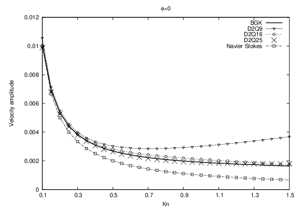
Although the standard LB model (D2Q9) is not sufficiently accurate in comparison with the DVM solution, high-order LB model (D2Q16) with minimal increase of the discrete velocity set can produce good results. Fig.1 shows that the LB model with increasing order of the Gauss-Hermite quadrature can closely approximate the linearized BGK equation. Therefore, in comparison with the DVM simulation, LB method can provide a practical engineering design simulation tool which can produce reasonably accurate results with significantly reduced computational cost.
As discussed in Section 2.3, at least three factors will influence the problem-solving process, i.e. the numerical scheme for solving Eq.(13), the order of Hermite expansion and Gauss-Hermite quadrature. For the numerical scheme, our second-order scheme is essential as discussed in Section 2.2. Regarding the role of Hermite expansion and Gauss-Hermite quadrature, we have theoretically proved that the Gauss-Hermite quadrature rather than the order of Hermite expansion is key to capturing non-equilibrium effects accurately. The numerical simulations have also performed to testify our theoretical analysis.
In Figs.2 and 3, the simulation results of the three LB models are compared with the solutions of directly solving the linearized BGK equation and the Navier Stokes equation. The expansion of the equilibrium distribution function and the forcing term is second-order for the D2Q9 model, third-order for the D2Q16 and forth-order for D2Q25. The results in Fig.2 show that the prediction for velocity amplitude of the D2Q25 model are in excellent agreement with the DVM solution of the linearized BGK equation across a broad range of Knudsen number () for the quasi-steady and time-varying problems with up to . Meanwhile, the results of the D2Q9 model deviate from the DVM solution of the linearized BGK equation significantly. Surprisingly, the D2Q9 model does not agree with the results predicted by the Navier Stokes equation. Fig.3 shows the velocity wave phase lag, which suggests that high-order LB models perform better in the transition flow regime.
Although Figs.2 and 3 demonstrate that increasing order of LB model in terms of the Hermite expansion and Gauss-Hermite quadrature will lead to more accurate results, we still do not know the exact role the orders of the Hermite expansion and the Gauss-Hermite quadrature play. Therefore, we single out the effect of the Hermite expansion in Fig.4, where the results of the LB models with the same quadrature but different Hermite expansion order are compared. The results clearly show that the Hermite expansion order for both the force and the equilibrium distribution function make negligible difference to the simulation results. Even the first order expansion is sufficient to obtain accurate velocity for the D2Q25 model. The simulation results support our theoretical analysis that the Hermite expansion has no direct influence on model accuracy for capturing non-equilibrium effects. Specifically, the LB model equation determined by the first order Hermite expansion is sufficient for a typical gas flow in micro-devices where the Mach number is usually small. In contrast, the Gauss-Hermite quadrature determines the model accuracy as the higher-order quadratures give better results.
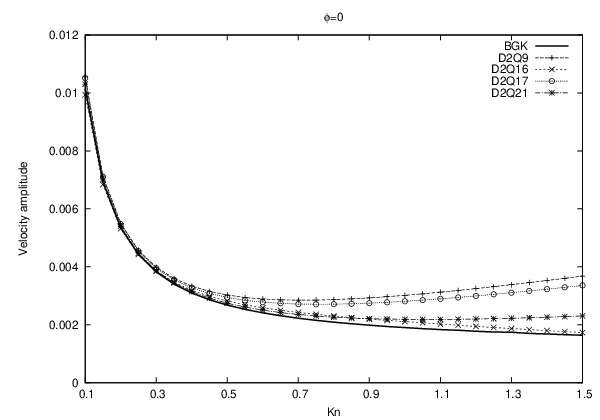
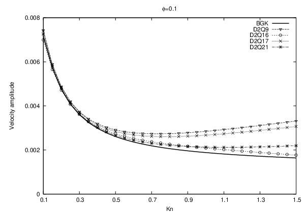
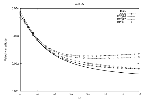
Not only the order of quadrature but also the abscissae may influence the model accuracy. Therefore, the simulation results of the three LB models with the same order quadrature but different abscissae are compared in Fig.5. Although increasing quadrature order will lead to improved accuracy, more discrete velocities may not improve the model performance if the quadratures are the same order. For example, the quadratures of the D2Q16, D2Q17 and D2Q21 models are the same order. Surprisingly, the D2Q16 model produces the results better than the other two models with more discrete velocities. The reason may be attributed to that the abscissae of the D2Q16 model has better symmetry. In addition, all these models are better than the D2Q9 model which has low order quadrature. Therefore, appropriate abscissae may improve the model accuracy and reduce the computational costs with smaller number of discrete velocities.
Since Lockerby & Reese (2008) has shown that the R13 equation gives the best performance among the extended hydrodynamic models, we compare the LB models with the R13 model here. Fig.6 shows that, in comparison with the data obtained from directly solving the linearized BGK equation, the high-order LB models including the D2Q16 and D2Q25 models can give better results than the R13 equation over a broad range of Knudsen numbers. Therefore, the high-order LB models with modest number of discrete velocity set, such as the D2Q16 and D2Q25 models, can offer close approximation to the linearized BGK equation. Most importantly, these high-order LB models achieve such degree of accuracy at a fraction of computational costs associated with directly solving the linearized BGK equation.
5 Concluding remarks
We have theoretically and numerically analyzed the high-order LB models for rarefied gas flows. The lattice Boltzmann equation is shown to be equivalent to the linearized BGK equation in the incompressible limit. When the same Gauss-Hermite quadrature is used, both LB and DVM simulations produce results in excellent agreement across a broad range of the Knudsen numbers. This suggests the importance of the Gauss-Hermite quadrature and the great potential of the LB method for modeling rarefied gas flows. While the Gauss-Hermite quadrature is of the most importance to capturing non-equilibrium effects, the first-order Hermite expansion on the equilibrium distribution function is sufficient to obtain the correct moments for isothermal flows e.g. increasing the Hermite expansion order further will not improve the model accuracy. For the same order Gauss-Hermite quadratures, the chosen abscissae will influence the model accuracy and more discrete velocities may not lead to improved model accuracy.
Overall, we have demonstrated that LB method offers a computationally efficient approach to solve the BGK equation. We can choose a suitable LB model to meet different requirement on model accuracy and computational efficiency, which offers an ideal flexible engineering design simulation tool to be able to simulate flows in the continuum and transition regimes.
6 Acknowledgments
The authors would like to thank Jason Reese, Xiaojun Gu and Guihua Tang for many informative discussions. This work was financially supported by the Engineering and Physical Sciences Research Council U.K. under Grants No. EP/D07455X/1 and No. EP/ F028865/1.
References
- Al-Ghoul & Chan Eu (2004) Al-Ghoul, M. & Eu, B. C. 2004 Generalized hydrodynamics and microflows. Phys. Rev. E 70 (1), 016301.
- Ansumali et al. (2007) Ansumali, S., Karlin, I. V., Arcidiacono, S., Abbas, A. & Prasianakis, N. I. 2007 Hydrodynamics beyond Navier-Stokes: Exact solution to the lattice Boltzmann hierarchy. Phys. Rev. Lett. 98 (12), 124502.
- Aoki et al. (1991) Aoki, K., Nishino, K., Sone, Y. & Sugimoto, H. 1991 Numerical analysis of steady flows of a gas condensing on or evaporating from its plane condensed phase on the basis of kinetic theory: Effect of gas motion along the condensed phase. Phys. Fluids A 3 (9), 2260–2275.
- Aoki et al. (2002) Aoki, K., Takata, S. & Nakanishi, T. 2002 Poiseuille-type flow of a rarefied gas between two parallel plates driven by a uniform external force. Phys. Rev. E 65 (2), 026315.
- Balakrishnan (2004) Balakrishnan, R. 2004 An approach to entropy consistency in second-order hydrodynamic equations. J. Fluid Mech. 503, 201–245.
- Benzi et al. (1992) Benzi, R., Succi, S. & Vergassola, M. 1992 The lattice Boltzmann equation: Theory and applications. Phys. Rep. 222, 145–197.
- Chapman & Cowling (1991) Chapman, S. & Cowling, T. G. 1991 The Mathematical Theory of Non-uniform Gases. Cambridge University Press.
- Chen & Doolen (1998) Chen, S. & Doolen, G. D. 1998 Lattice Boltzmann method for fluid flows. Annu. Rev. Fluid Mech. 30, 329–364.
- Chikatamarla & Karlin (2006) Chikatamarla, S. S. & Karlin, I. V. 2006 Entropy and Galilean invariance of lattice Boltzmann theories. Phys. Rev. Lett. 97 (19), 190601.
- He et al. (1998) He, X. Y., Chen, S. Y. & Doolen, G. D. 1998 A novel thermal model for the lattice Boltzmann method in incompressible limit. J. Comput. Phys. 146 (1), 282 – 300.
- He & Luo (1997a) He, X. Y. & Luo, L. S. 1997a A priori derivation of the lattice Boltzmann equation. Phys. Rev. E 55 (6), R6333–R6336.
- He & Luo (1997b) He, X. Y. & Luo, L. S. 1997b Theory of the lattice Boltzmann method: From the Boltzmann equation to the lattice Boltzmann equation. Phys. Rev. E 56 (6), 6811–6817.
- He et al. (1996) He, X. Y., Luo, L. S. & Dembo, M. 1996 Some progress in lattice Boltzmann method. part i. nonuniform mesh grids. J. Comput. Phys. 129 (2), 357–363.
- Ho & Tai (1998) Ho, C. M. & Tai, Y. C 1998 Micro-electro-mechanical-systems (MEMS) and fluid flows. Annu. Rev. Fluid Mech. 30 (1), 579–612.
- Kim et al. (2008) Kim, S. H., Pitsch, H. & Boyd, I. D. 2008 Accuracy of higher-order lattice Boltzmann methods for microscale flows with finite Knudsen numbers. J. Comput. Phys. 227 (19), 8655 – 8671.
- Lim et al. (2002) Lim, C. Y., Shu, C., Niu, X. D. & Chew, Y. T. 2002 Application of lattice Boltzmann method to simulate microchannel flows. Phys. Fluids 14 (7), 2299–2308.
- Lockerby & Reese (2008) Lockerby, D. A. & Reese, J. M. 2008 On the modelling of isothermal gas flows at the microscale. J. Fluid Mech. 604, 235–261.
- Luo (2000) Luo, L. S. 2000 Some recent results on discrete velocity models and ramifications for lattice Boltzmann equation. Comput. Phys. Commun. 129 (1-3), 63 – 74.
- Mieussens (2000a) Mieussens, L. 2000a Discrete velocity model and implicit scheme for the BGK equation of rarefied gas dynamics. Math. Models Methods Appl. 10, 1121–1149.
- Mieussens (2000b) Mieussens, L. 2000b Discrete-velocity models and numerical schemes for the Boltzmann-BGK equation in plane and axisymmetric geometries. J. Comput. Phys. 162 (2), 429 – 466.
- Mieussens (2001) Mieussens, L. 2001 Convergence of a discrete-velocity model for the Boltzmann-BGK equation. Comput. Math. Appl 41 (1-2), 83 – 96.
- Naris & Valougeorgis (2005) Naris, S. & Valougeorgis, D. 2005 The driven cavity flow over the whole range of the Knudsen number. Phys. Fluids 17 (9), 097106.
- Naris et al. (2005) Naris, S., Valougeorgis, D., Kalempa, D. & Sharipov, F. 2005 Flow of gaseous mixtures through rectangular microchannels driven by pressure, temperature, and concentration gradients. Phys. Fluids 17 (10), 100607–12.
- Nie et al. (2002) Nie, X. B., Doolen, G. D. & Chen, S. Y. 2002 Lattice-Boltzmann simulations of fluid flows in mems. J. Stat. Phys. 107 (1), 279–289.
- Qian et al. (1992) Qian, Y. H., D’Humières, D. & Lallemand, P. 1992 Lattice BGK models for Navier-Stokes equation. Europhys. Lett. 17 (6), 479–484.
- Reider & Sterling (1995) Reider, M. B. & Sterling, J. D. 1995 Accuracy of discrete-velocity BGK models for the simulation of the incompressible Navier-Stokes equations. Comput. Fluids 24 (4), 459 – 467.
- Sbragaglia & Succi (2005) Sbragaglia, M. & Succi, S. 2005 Analytical calculation of slip flow in lattice Boltzmann models with kinetic boundary conditions. Phys. Fluids 17 (9), 093602.
- Sbragaglia & Succi (2006) Sbragaglia, M. & Succi, S. 2006 A note on the lattice Boltzmann method beyond the Chapman-Enskog limits. Europhys. Lett. 73 (3), 370–376.
- Shan & He (1998) Shan, X. W. & He, X. Y 1998 Discretization of the velocity space in the solution of the Boltzmann equation. Phys. Rev. Lett. 80 (1), 65–68.
- Shan et al. (2006) Shan, X. W., Yuan, X. F. & Chen, H. D. 2006 Kinetic theory representation of hydrodynamics: a way beyond the Navier Stokes equation. J. Fluid Mech. 550, 413–441.
- Sharipov & Bertoldo (2009) Sharipov, F. & Bertoldo, G. 2009 Numerical solution of the linearized Boltzmann equation for an arbitrary intermolecular potential. J. Comput. Phys. 228 (9), 3345 – 3357.
- Sharipov & Kalempa (2008) Sharipov, F. & Kalempa, D. 2008 Oscillatory couette flow at arbitrary oscillation frequency over the whole range of the knudsen number. Microfluid. Nanofluid. 4 (5), 363–374.
- Sterling & Chen (1996) Sterling, J. D. & Chen, S. Y. 1996 Stability analysis of lattice Boltzmann methods. J. Comput. Phys. 123 (1), 196–206.
- Struchtrup & Torrilhon (2003) Struchtrup, H. & Torrilhon, M. 2003 Regularization of Grad’s 13 moment equations: Derivation and linear analysis. Phys. Fluids 15 (9), 2668–2680.
- Tang et al. (2008) Tang, G. H., Zhang, Y. H. & Emerson, D. R. 2008 Lattice Boltzmann models for nonequilibrium gas flows. Phys. Rev. E 77 (4), 046701.
- Toschi & Succi (2005) Toschi, F. & Succi, S. 2005 Lattice Boltzmann method at finite Knudsen numbers. Europhys. Lett. 69 (4), 549–555.
- Valougeorgis (1988) Valougeorgis, D. 1988 Couette flow of a binary gas mixture. Phys. Fluids 31 (3), 521–524.
- Yang & Huang (1995) Yang, J. Y. & Huang, J. C. 1995 Rarefied flow computations using nonlinear model Boltzmann equations. J. Comput. Phys. 120 (2), 323 – 339.
- Yudistiawan et al. (2008) Yudistiawan, W. P., Ansumali, S. & Karlin, I. V. 2008 Hydrodynamics beyond Navier-Stokes: The slip flow model. Phys. Rev. E 78 (1), 016705.
- Zhang et al. (2005) Zhang, Y. H., Qin, R. S. & Emerson, D. R. 2005 Lattice Boltzmann simulation of rarefied gas flows in microchannels. Phys. Rev. E 71 (4), 047702.
- Zhang et al. (2006) Zhang, Y. H., Gu, X. J., Barber, R. W. & Emerson, D. R. 2006 Capturing Knudsen layer phenomena using a lattice Boltzmann model. Phys. Rev. E 74 (4), 046704.
- Zhong et al. (1993) Zhong, X. L., Chapman, D. R. & MacCormack, R. W. 1993 Stabilization of the Burnett equations and application to hypersonicflows. AIAA Journal 31, 1036–1043.