Few-Qubit Lasing in circuit QED

The “SSET laser” realized by Astafiev et al. [12] consists of an SSET coupled capacitively to a microstripline resonator, as shown in Fig. 1a. The properties of the coupled system and the specific form of the Hamiltonian will be analyzed further in later Sections and in Appendix A. In the present Section we describe how a population inversion is created in a suitably biased SSET.

A superconducting single-electron transistor (SSET) consists of two superconducting leads coupled by tunnel junctions to a superconducting island. A gate voltage $U$ shifts the electrostatic energy of the island and controls, together with the bias voltage $V$, the current through the device. The Josephson coupling, $E_{\rm J}$, allowing for coherent Cooper pair tunneling through the junctions, is weak compared to the superconducting energy gap $\Delta_{sc}$ and to the charging energy of the island, $E_{C}=e^{2}/2C$, $C$ being the total island’s capacitance. In addition, quasiparticles can tunnel incoherently (with rate $\propto V/eR$, where $R$ is the resistance of the tunnel junction) when the energy difference between initial and final states is sufficient to create a quasiparticle excitation, i.e., when it exceeds twice the gap, $|\Delta E|\geq 2\Delta_{sc}$. We denote by $N$ the number of excess charges on the island; it changes by $\pm 1$ in a single-electron tunneling process and by $\pm 2$ in a Cooper pair tunneling event. At low temperatures for the conditions realized experimentally the number of accessible charge states of the island is strongly reduced. For the further calculations we can restrict our analysis to $N=0,1,2$.

We assume the SSET to be tuned close to the Josephson quasiparticle (JQP) cycle, where the current is transported by a combination of Cooper pair tunneling through one junction and two consecutive quasiparticle tunneling events through the other junction. The parameters of the junctions are chosen asymmetrically. By changing the transport voltage $V$ and the gate voltage $U$, we can tune to a situation, where resonant Cooper pair tunneling is strong across, say, the lower junction, while quasiparticle tunneling is strong across the upper one. Specifically, when the normalized “gate charge” $N_{\rm G}=C_{\rm G}U/e$ is approximately $1$, $N_{\rm G}\approx 1$, the charge states $|N=0\rangle$ and $|N=2\rangle$ are near degeneracy with respect to coherent Cooper pair tunneling across the lower junction. Hence the eigenstates are

where $\tan\xi=E_{\rm J}/\epsilon_{ch}$ with $\epsilon_{ch}=4(N_{\rm G}-1)E_{C}$. Quasiparticle tunneling across the upper junction leads to transitions between the states $|\uparrow\rangle$ and $|\downarrow\rangle$ and the odd charge state $|N=1\rangle$. The transition rates are

The dependence on the relevant matrix elements and the energy gain $eV$ can be lumped into the function $I(V)$, which is the normal current through the junction at voltage $V$. Here we can assume that the relevant energy scale for each tunnel event is the applied voltage and neglect the smaller change of the energy of the island.

By choosing $\xi$ such that $\cos\frac{\xi}{2}>\sin\frac{\xi}{2}$, we can create a population inversion. In this case, the quasiparticle tunneling processes (2) leading from $|\downarrow\rangle$ via $|1\rangle$ to $|\uparrow\rangle$ become stronger than the processes in opposite direction (see fig. 1b)). From the transition rates (2) we readily obtain the bare population inversion in the system,

where $\rho_{ii}$ is the population of the state $|i\rangle$ with $i=\uparrow,\,\downarrow$.

In this subsection we consider systems as investigated in Ref. [2, 13] and shown in Fig. 2.

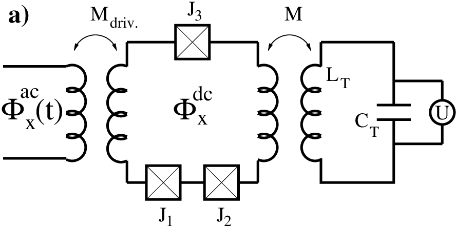
Here, a flux qubit is strongly driven by $ac$-fields to perform Rabi oscillations. It is further coupled to a low-frequency $LC$-oscillator. In the strongly driven situation the physics is most conveniently described in the basis of “dressed states” in the rotating frame [17]. The transformation to dressed states modifies the relaxation, excitation and decoherence rates as compared to the standard results [18, 19]. As a result, for blue detuning of the driving frequency compared to the resonant frequency a population inversion is produced in the dressed state basis, which in turn can lead to lasing [20].

To illustrate these effects we first consider the driven qubit (ignoring the coupling to the resonator) coupled to a bath observable $\hat{X}$,

In the absence of driving, $\Omega_{\rm R0}=0$, and for regular (i.e., smooth as function of the frequency) power spectra of the fluctuating bath observables we can proceed using Golden rule type arguments [18, 19]. The transverse noise, coupling to $\sigma_{x}$ and $\sigma_{y}$, is responsible for relaxation and excitation processes with rates

while longitudinal noise, coupling to $\sigma_{z}$, produces a pure dephasing with rate

Here $b_{\perp}\equiv b_{x}+ib_{y}$, and we introduced the ordered correlation function $\langle\hat{X}^{2}\rangle_{\omega}\equiv\int dt\ e^{i\omega t}\langle\hat{X}(t)\hat{X}(0)\rangle$, as well as the power spectrum, i.e., the symmetrized correlation function, $S_{X}(\omega)\equiv(\langle\hat{X}^{2}\rangle_{\omega}+\langle\hat{X}^{2}\rangle_{-\omega})/2$. The rates (5) and (6) also define the relaxation rate $1/T_{1}=\Gamma_{1}=\Gamma_{\downarrow}+\Gamma_{\uparrow}$ and the total dephasing rate $1/T_{2}=\Gamma_{\varphi}=\Gamma_{1}/2+\Gamma_{\varphi}^{*}$ which appear in the Bloch equations for the qubit.

To account for the driving with frequency $\omega_{d}$ it is convenient to transform to the rotating frame via a unitary transformation $U_{r}=\exp{(-i\omega_{d}\,\sigma_{z}t/2)}$. Within rotating-wave approximation (RWA) the transformed Hamiltonian reduces to

with detuning $\delta\omega\equiv\omega_{d}-\Delta E/\hbar$. The RWA cannot be used in the second line of (7) since the fluctuations $\hat{X}$ contain potentially frequencies close to $\pm\omega_{d}$, which can compensate fast oscillations. Diagonalizing the first two terms of (7) one obtains

where the full Rabi frequency is $\Omega_{\rm R}=\sqrt{\Omega_{\rm R0}^{2}+\delta\omega^{2}}$, and the detuning determines the parameter $\beta$ via

From here Golden-rule arguments lead to the relaxation and excitation rates in the rotating frame as well as the ”pure” dephasing rate [21]

We note the effect of the frequency mixing. In addition, due to the diagonalization the effects of longitudinal and transverse noise on relaxation and decoherence get mixed. We further note that the rates also depend on the fluctuations’ power spectrum at the Rabi frequency, $\langle\hat{X}^{2}\rangle_{\pm\Omega_{\rm R}}$.

For a sufficiently regular power spectrum of the fluctuations at frequencies $\omega\approx\pm\Delta E/\hbar$ we can ignore the effect of detuning and the small shifts by $\pm\Omega_{\rm R}$ as compared to the high frequency $\omega_{d}\approx\Delta E/\hbar$. We further assume that $\Omega_{\rm R}\ll kT/\hbar$. In this case we find the simple relations

where the rates in the lab frame are given by Eqs. (5,6) and the new rate

depends on the power spectrum at the Rabi frequency.

To proceed we concentrate on the most relevant regime. At low temperatures, $k_{\rm B}T\ll\Delta E\approx\hbar\omega_{d}$, we can neglect $\Gamma_{\uparrow}$ as it is exponentially small. We also assume that $\Gamma_{\nu}$ can be neglected as compared to $\Gamma_{\downarrow}$, which is justified, e.g., when the qubit is tuned close to the symmetry point where $b_{z}\ll|b_{\perp}|$. Since the rate $\Gamma_{\nu}$ depends on the noise power spectrum at the frequency $\Omega_{\rm R}$, which is usually higher that the frequency range of the $1/f$ noise, the latter does not change the situation. Thus we neglect $\Gamma_{\nu}$ and we are left with

The ratio of up- and down-transitions depends on the detuning and can be expressed by an effective temperature. Right on resonance, where $\beta=0$, we have $\tilde{\Gamma}_{\uparrow}=\tilde{\Gamma}_{\downarrow}$, corresponding to infinite temperature or a classical drive. For “blue” detuning, $\beta>0$, we find $\tilde{\Gamma}_{\uparrow}>\tilde{\Gamma}_{\downarrow}$, i.e., negative temperature. This leads to a population inversion of the qubit, which is the basis for the lasing behavior which will be described below.

In a more careful analysis, paying attention to the small frequency shifts by $\pm\Omega_{\rm R}$, we obtain for $\beta=0$

For example, for Ohmic noise and low bath temperature this reduces to $\tilde{\Gamma}_{\downarrow}/\tilde{\Gamma}_{\uparrow}\approx 1+2\Omega_{\rm R}/\omega_{d}$, which corresponds to an effective temperature of order $2\hbar\omega_{d}/k_{\rm B}\approx 2\Delta E/k_{\rm B}$, which by assumption is high but finite. The infinite temperature threshold is crossed toward negative temperatures at weak blue detuning when the condition

is satisfied. We note that all qualitative features are well reproduced by the approximation (13).

To illustrate the calculations outlined above and the mechanism creating the population inversion for blue detuning we show in Fig. 3 the level structure, i.e., the formation of dressed states, of a near-resonantly driven qubit. For the purpose of the present discussion we assume that also the driving field is quantized. This level structure was described first by Mollow [17]. The picture also illustrates how for blue detuning a pure relaxation process, $\Gamma_{\downarrow}$, in the laboratory frame predominantly leads to an excitation process, $\tilde{\Gamma}_{\uparrow}$, in the rotating frame, thus creating a population inversion in the basis of “dressed states”.

If this effective inverted two-state system is coupled to an oscillator, a lasing state is induced. In Ref. [20] it was proposed to couple the oscillator to the dressed states belonging to the neighboring doublets (see Fig. 3). Then, to be in resonance with the pair of dressed states with population inversion the oscillator frequency should satisfy $\omega_{0}=\omega_{d}+\Omega_{\rm R}$. As $\omega_{d}\sim\Delta E$ and $\Omega_{\rm R}\ll\Delta E$ this can work for a high-frequency resonator approximately in resonance with the qubit, $\omega_{0}\approx\Delta E$. In contrast, in Ref. [22] a different situation was considered where the oscillator was coupled to the dressed states belonging to the same doublet. The resonance condition then reads $\omega_{0}=\Omega_{\rm R}$, and the lasing can be reached for an oscillator much slower than the qubit, $\omega_{0}\ll\Delta E$, which is the situation realized in Ref. [2]. An additional complication arises at the symmetry point of the qubit, since there the single-photon coupling between the oscillator and the doublet of the dressed states vanishes. Then, two-photon processes become relevant with the resonance condition $2\omega_{0}=\Omega_{R}$ [22].

Factorizing the correlator, $\langle S_{z}n\rangle\approx\langle S_{z}\rangle\langle n\rangle$, on the right-hand side of Eqs. (22) and neglecting the qubit-qubit correlations, $C_{QQ}\simeq 0$, we reproduce results known in quantum optics as “semi-quantum model” [16]. This approximation yields a quadratic equation for the scaled average photon number (per qubit) $\tilde{n}=\langle n\rangle/N_{a}$,

which depends on the parameter $\tilde{n}_{0}=\frac{\Gamma_{1}\gamma}{4g^{2}N_{a}}\left(1+\frac{\Delta^{2}}{\gamma^{2}}\right)$. This equation has always one positive solution $\tilde{n}>0$.

Before continuing the analysis of the properties of the semi-quantum solution, for sake of comparison, we recall the standard semiclassical results. In this approximation the operator $a$ is treated as a classical stochastic variable, $\alpha$. After adiabatic elimination of the qubits’ degrees of freedom, i.e., assuming $\Gamma_{\varphi}\gg\kappa/2$, one obtains a classical Langevin equation for $\alpha$,

Here $\xi(t)$ is a classical Langevin force due to thermal noise, $\langle\xi(t)\xi^{*}(t^{\prime})\rangle=\kappa N_{\rm th}\delta(t-t^{\prime})$, and $s_{z}^{\rm st}=D_{0}/(1+\left|\alpha\right|^{2}/(\tilde{n}_{0}N_{a}))$ denotes the stationary qubits’ polarization.

In order to obtain an expression for the average photon number $\langle n\rangle=\langle\left|\alpha\right|^{2}\rangle$ we rewrite the Langevin equation as $\dot{\alpha}=-f(\left|\alpha\right|^{2})\alpha+\xi(t)$ and approximate $\langle f(\left|\alpha\right|^{2})\cdot\left|\alpha\right|^{2}\rangle\approx f(\langle n\rangle)\cdot\langle n\rangle$. Thus we arrive at the equation $\frac{d}{dt}\langle n\rangle=-2\mathrm{\rm Re}\{f(\langle n\rangle)\}\cdot\langle n\rangle+\kappa N_{\rm th}$, from which we obtain in the steady state a quadratic equation for the scaled photon number $\tilde{n}=\langle n\rangle/N_{a}$,

In the low-temperature limit, $N_{\rm th}\sim 0$, the semiclassical results can be rewritten in the simple form, $\tilde{n}^{2}+\left(\tilde{n}_{0}-\Gamma_{1}D_{0}/2\kappa\right)\tilde{n}\approx 0$, with $\tilde{n}_{0}=\frac{\Gamma_{1}\Gamma_{\varphi}}{4g^{2}N_{a}}\left(1+\frac{\Delta^{2}}{\Gamma_{\varphi}^{2}}\right)$. This gives the well-known threshold condition $D_{0}>\kappa\Gamma_{\varphi}/(2g^{2}N_{a})$ for the lasing state.

Different from the semiclassical picture, the semi-quantum model includes the effects of spontaneous emission processes, described by the term proportional to $(\langle S_{z}\rangle+1)$ in Eqs. (22). Spontaneous emission is responsible for the linewidth of the lasers, and, as noticed in Ref. [27], due to the low photon number, spontaneous emission is especially relevant for the dynamics of single-atom lasers.

To illustrate the effect of spontaneous emission on the lasing transition and at the same time the quality of the semi-quantum approximation, we plot the photon number as a function of the coupling strength $g$ for $N_{a}=1$ (Fig. 4, left panel) and $N_{a}=2$ (Fig. 4, rigth panel). The plots show the semi-quantum, semiclassical and Master equation results. We note that the semi-quantum approximation gives results in very good agreement with the Master equation. Moreover, both the semi-quantum and Master equation solution show a smooth crossover between the normal and the lasing regimes, an effect which is due to spontaneous emission. While we cannot define a sharp threshold condition, we can still identify, even for a single-atom laser, a well localized transition region centered at the threshold coupling predicted by the semiclassical approximation.

In the left panel of Fig. 4 we also plot the qubit-oscillator correlator, $\langle S_{z}n\rangle$, and the factorized approximation, $\langle S_{z}\rangle\langle n\rangle$. For strong coupling, they differ significantly. However, as the good agreement between the semi-quantum approximation and the numerical solution of the Master equation demonstrates, the qubit-field correlations have only a weak effect on the average photon number. On the other hand, as we will see in the following section, the qubit-field correlations have an important effect on the spectral properties of the single-qubit laser.

The right panel of Fig. 4, shows the qubit-qubit correlations $C_{QQ}$ for a two-qubit-laser. Similar as the qubit-field correlations, they are neglected in the semi-quantum approximation. Both correlations are maximum at the lasing transition, but decay away from this point. The reason is that qubit-field and qubit-qubit correlations scale as $g^{2}/\Gamma_{\varphi}^{2}$, thus they are small for weak coupling. On the other hand, they are proportional to the qubit inversion $\langle S_{z}\rangle$ and hence vanish rapidly above the transition.

Similarly to Eqs. (21) for the average values, we can derive equations for the laser and cross correlation functions, $O(\tau)$ and $G(\tau)=\lim_{t\rightarrow\infty}\langle\sigma_{+}(t+\tau)a(t)\rangle$. Assuming that the oscillator damping is much weaker than the qubits’ dephasing, $\kappa/2\ll\Gamma_{\varphi}$, which is usually satisfied in single-qubit lasing experiments, we obtain a single equation for the oscillator correlation function: $\frac{d}{d\tau}\langle a^{\dagger}(t+\tau)a(t)\rangle=\left(i\omega_{0}-\kappa/2\right)\langle a^{\dagger}(t+\tau)a(t)\rangle+g^{2}/\Gamma_{\varphi}\langle\sigma_{z}\rangle\langle a^{\dagger}(t+\tau)a(t)\rangle$. Thus the semi-quantum theory predicts an exponential decay of the correlation function $O(\tau)$, which corresponds to a Lorentzian shape of the emission spectrum,

where the width of the spectrum is given by the expression

For the following discussion we focus on the case of a single qubit, $N_{a}=1$. In the left panel of Fig. 5 we plot the diffusion constant $\kappa_{d}$, as function of the coupling strength $g$, covering the whole range from below to above the transition, and compare it to the diffusion constant $\kappa_{d}^{\rm fac}$, obtained from the semi-quantum theory, i.e., by neglecting the qubit-field-correlations $\langle\sigma_{z}n\rangle-\langle\sigma_{z}\rangle\langle n\rangle$.

Upon approaching the broadened lasing threshold from the weak coupling side we observe the linewidth narrowing characteristic for the lasing transition. However, above the transition, the linewidth increases again with growing coupling strength, thus deteriorating the lasing state. By comparing the semi-quantum approximation with the full solution of the master equation, we observe that qubit-oscillator correlations have a significant quantitative effect on the phase diffusion, leading to a reduction of the linewidth by roughly a factor $1/2$, but they do not change the qualitative conclusions.

Also in Fig. 5, we note that in the transition region there is an “optimal” value of the qubit-oscillator coupling where the height of the spectral line, which is given by the ratio $\langle n\rangle/\kappa_{d}$ of the photon number and the linewidth, is maximum. This interesting feature is due to the fact that in single- and few-qubit lasers far above the lasing transition a increase of the coupling has little effect on the saturated photon number, but leads to an increase of the incoherent photon emission rate and the linewidth.

When the qubit and the resonator are not in resonance, $\Delta\neq 0$, the emission spectrum is shifted with respect to the natural frequency $\omega_{0}$ of the resonator. This is shown in the right panel of figure 5 where we plot the average photon number, the linewidth and the frequency shift $\delta\omega_{0}$ as functions of the detuning $\Delta$ in the strong coupling regime.

The numerical results for the linewidth $\kappa_{d}$ shown in this plot differ qualitatively from the results presented in our previous paper [15], where we use a factorization scheme to obtain analytical expressions for the linewidth. Specifically, moving away from the resonance the linewidth is increasing, while the factorization predicted a decrease. On the other hand, the approximation based on the factorization yields results very similar to the numerical ones right on resonance, as well as in the far off-resonant situation and the weak-coupling regime.

As discussed in a quantum optics context in Refs. [27, 28], various properties of single qubit masers are due to the fact that in these systems only one artificial atom (a microscopic system from a thermodynamical point of view) interacts with the electromagnetic radiation. To clarify the main differences between single qubit masers and conventional (many atom) lasers, we use the semi-quantum approximation to study the scaling of the average photon number and of the phase diffusion with the number of atoms.

In Fig. 6, we plot the scaled photon number $\langle n\rangle/N_{a}$ in the transition region and $\kappa_{d}$ versus the scaled coupling, $g\sqrt{N_{a}}$, for different values of the number of qubits $N_{a}$. Plotted in these scaled forms, all curves have the same asymptotic behavior, and the transition occurs at the same position. As expected, in Fig. 6 (left panel) we observe that for low values of $N_{a}$, there is a smoothening of the lasing transition which is due to spontaneous emission processes and disappears in the large $N_{a}$ limit. In Fig. 6 (right panel) we show the scaling of the phase diffusion constant. Here the qubits’ relaxation processes are responsible for the increase of the phase diffusion rate in the case of strong qubit-oscillator coupling for small $N_{a}$.

The linewidth of order of 0.3MHz observed in Ref. [12] is about one order of magnitude larger than what follows from our results (of the order of the Schawlow-Townes linewidth). Moreover, in the experiment, the emission spectrum shows a Gaussian rather than a Lorentzian shape. Both discrepancies can be explained if we note that the qubits’ dephasing is mostly due to low-frequency charge noise, which cannot be treated within the Markov approximation used in the present analysis.

However, low-frequency (quasi-static) noise can be taken into account by averaging the Lorentzian spectral line over different values of the energy splitting $\epsilon$ of the qubit [30], or equivalently, over different values of the detuning $\Delta$ between qubit and oscillator. Assuming that these fluctuations are Gaussian distributed, with mean $\bar{\Delta}$ and width $\sigma$, such that $\Gamma_{1}>\sigma\gg\kappa_{d}$, we can neglect in the saturated limit the dependence of $\kappa_{d}$ and $\langle n\rangle$ on $\Delta$ and assume that the frequency shift $\delta\omega_{0}$ depends linearly on the detuning $\Delta$.

In the strong coupling regime, the shift of the emission spectrum is given, in a good approximation, by $\delta\omega_{0}\simeq\Delta\kappa/(2\Gamma_{\varphi})$, which leads to a Gaussian line of width $\tilde{\sigma}\simeq\sigma\kappa/(2\Gamma_{\varphi})$, where we remark that $\Gamma_{\varphi}$ is the total Markovian dephasing rate. In this way, the linewidth observed in the experiment can be reproduced by a reasonable choice of $\sigma$ of order of 300 MHz. In the case in which $\sigma$ is larger than $\Gamma_{1}$, the previous formula overestimates the linewidth since it does not take into account the decay of $\langle n\rangle$ below the lasing transition. In this case we can still perform the averaging numerically. In either case we note that in the presence of low-frequency noise, the linewidth is governed not by $\kappa_{d}$, but by $\delta\omega_{0}$.

References

- [1] A. Blais et al., Phys. Rev. A 69, 062320 (2004); R. Schoelkopf and S. Girvin, Nature 451, 664 (2008).
- [2] E. Il’ichev et al., Phys. Rev. Lett. 91, 097906 (2003).
- [3] A. Wallraff et al., Nature 431, 162 (2004).
- [4] I. Chiorescu et al., Nature 431, 159 (2004).
- [5] G. Johansson, L. Tornberg, and C. M. Wilson, Phys. Rev. B 74, 100504 (2006).
- [6] M. A. Sillanpää, J. I. Park, and R. W. Simmonds, Nature 449, 438 (2007); J. Majer et al., Nature 449, 443 (2007).
- [7] P.J. Leek et al., Science 318, 1889 (2007).
- [8] S. Filipp et al., Phys. Rev. Lett. 102, 200402 (2009)); P.J. Leek et al., Phys. Rev. B 79, 180511(R) (2009).
- [9] L. Di Carlo et al., Nature 460, 240 (2009).
- [10] M. Hofheinz et al., Nature 454, 310 (2008); J. M. Fink et al., Nature 454, 315 (2008).
- [11] M. A. Sillanpää et al., arxiv: 0904.2553 (2009).
- [12] O. Astafiev et al., Nature 449, 588 (2007).
- [13] M. Grajcar et al., Nature Physics 4, 612 (2008).
- [14] H. Haken, Laser Theory, Springer, Berlin, 1984.
- [15] S. André, V. Brosco, A. Shnirman, and G. Schön, Phys. Rev. A. 79, 053848 (2009)
- [16] P. Mandel, Phys. Rev. A 21, 2020 (1980).
- [17] B. R. Mollow, Phys. Rev. 188, 1969 (1969).
- [18] F. Bloch, Phys. Rev. 105, 1206 (1957).
- [19] A. G. Redfield, IBM J. Res. Dev. 1, 19 (1957).
- [20] J. Zakrzewski, M. Lewenstein, and T. W. Mossberg, Phys. Rev. A 44, 7717 (1991).
- [21] G. Ithier et al., Phys. Rev. B 72, 134519 (2005).
- [22] J. Hauss et al., Phys. Rev. Lett. 100, 037003 (2008).
- [23] M. Tavis and F.W. Cummings, Phys. Rev. 170, 379 (1968).
- [24] C. W. Gardiner and P. Zoller, Quantum Noise, Springer, Berlin, 2004.
- [25] C. Cohen-Tannoudji, J. Dupont-Roc, and G. Grynberg, Atom-Photon Interactions, (Wiley, New York, 1992).
- [26] S. Ashhab et al., New J. Phys. 11, 023030 (2009)
- [27] Y. Mu and C.M. Savage, Phys. Rev. A 46, 5944 (1992).
- [28] C. Ginzel et al., Phys. Rev. A 48, 732 (1993).
- [29] D.A. Rodrigues, J. Imbers, and A.D. Armour, Phys. Rev. Lett. 98, 067204 (2007).
- [30] G. Falci et al., Phys. Rev. Lett. 94, 167002 (2005).
- [31] Z. C. Wang and H. Haken, Z. Phys. B 55, 361 (1984).