Trapping in scale-free networks with hierarchical organization of modularity
Abstract
A wide variety of real-life networks share two remarkable generic topological properties: scale-free behavior and modular organization, and it is natural and important to study how these two features affect the dynamical processes taking place on such networks. In this paper, we investigate a simple stochastic process—trapping problem, a random walk with a perfect trap fixed at a given location, performed on a family of hierarchical networks that exhibit simultaneously striking scale-free and modular structure. We focus on a particular case with the immobile trap positioned at the hub node having the largest degree. Using a method based on generating functions, we determine explicitly the mean first-passage time (MFPT) for the trapping problem, which is the mean of the node-to-trap first-passage time over the entire network. The exact expression for the MFPT is calculated through the recurrence relations derived from the special construction of the hierarchical networks. The obtained rigorous formula corroborated by extensive direct numerical calculations exhibits that the MFPT grows algebraically with the network order. Concretely, the MFPT increases as a power-law function of the number of nodes with the exponent much less than 1. We demonstrate that the hierarchical networks under consideration have more efficient structure for transport by diffusion in contrast with other analytically soluble media including some previously studied scale-free networks. We argue that the scale-free and modular topologies are responsible for the high efficiency of the trapping process on the hierarchical networks.
pacs
05.40.Fb, 89.75.Hc, 05.60.Cd, 89.75.DaI Introduction
Complex networks are a powerful and versatile mathematical tool for representing and modeling structure of complex systems [1, 2], and their wide applications in different areas have made them become a subject of a large volume of research in the past decade [3, 4]. Within the general framework of complex networks, scientists can offer in qualitative terms the detailed microscopic description of structural properties and complexity of real-life systems. Extensive empirical analysis on diverse real systems has unveiled that many, perhaps most, real-world networks are simultaneously characterized by the two most remarkable features: scale-free behavior [5] and modular organization [6, 7, 8]. The scale-free nature of a network means that its degree distribution follows a power law as with the degree distribution exponent in the range of , while the modular organization implies that the network is formed by groups (modules) of nodes that have a significantly higher interconnection density compared to the overall density of the whole network. The important finding of these two fundamental natures has led to the rising of research on some outstanding issues in the field of complex networks such as exploring the generation mechanisms for scale-free behavior [1, 2], detecting and characterizing modular structure [9, 10, 11, 12], and so on. On the other hand, it has been shown that the two characteristics are closely related to other structural properties such as average path length [13, 14] and clustering coefficient [8].
In principle, one of the main reasons for studying structural properties of complex networks is to understand how the dynamical processes are influenced by the underlying topological structure [15]. Among a plethora of random processes, random walks with wide range of distinct applications to many science branches, have attracted a considerable amount of recent attention within the physics community [16, 17, 18, 19, 20, 21, 22, 23, 24, 25, 26, 27, 28, 29, 30, 31]. Particularly, trapping issue, an integral major theme of random walks, is relevant to a variety of contexts, including target research [32, 33], photon-harvesting processes in photosynthetic cells [34], and characterizing similarities between the elements of a database [35] has led to an increasing number of theoretical and practical investigations over the last several decades. Numerous authors have made concerted efforts to study trapping problem in different media, including regular lattices [36], Sierpinski fractals [37, 38], T fractal [39], small-world networks [40], and scale-free networks [41, 42, 43, 44, 45], as well as other structures [46, 47, 48]. These studies unclosed many unusual and exotic phenomena of trapping on diverse graphs. However, the trapping process on scale-free networks with modular structure remains less understood, in spite of the facts that modularity plays an important role in shaping up scale-free networks [49], and that taking into account the modular structure of scale-free networks leads to a better understanding of how the underlying systems work [50].
In this paper, we study the classic trapping problem on a class of hierarchical networks [7, 8], which is a random walk problem with a single immobile trap positioned at a given site, absorbing all walks visiting it. Here we focus on a particular case with the trap located at the node with the highest degree. The networks studied can capture simultaneously scale-free behavior and modular structure. Moreover, the networks belong to a deterministic growing type of networks, which have received much attention from the scientific communities and have proved to be a useful tool [51, 52, 53, 54, 55, 56, 57, 58, 59, 60, 61]. The deterministic nature of the hierarchical networks makes it possible to investigate analytically the trapping process defined on them. By applying the formalism [62, 63] of generating functions [64] for random walks, we derive the rigorous solution to the mean first-passage time (MFPT) that characterizes the trapping process. The obtained exact result shows that the MFPT scales algebraically with the number of network nodes. We also compare the behavior of the trapping problem on the hierarchical networks with those of other networks, and show that the hierarchical networks can be helpful for enhancing the efficiency of the trapping process.
II Modular scale-free networks
Let us introduce the model for the hierarchical scale-free networks with a modular structure, which can be constructed in an iterative way [7, 8]. We denote by the network model after () iterations (number of generations). Initially (), the network consists of a central node, called the hub (root) node, and peripheral (external) nodes with . All these initial nodes are fully connected to each other, forming a complete graph. At the second generation (), we generate copies of and connect the external nodes of each replica to the root of the original . The hub of the original and the peripheral nodes in the replicas become the hub and peripheral nodes of , respectively. Suppose one has , the next generation network can be obtained from by adding replicas of with their external nodes being linked to the hub of the original unit. In , its hub is the hub of the original , and its external nodes are composed of all the peripheral nodes of the copies of . Repeating indefinitely the replication and connection steps, we obtain the hierarchical modular scale-free networks. Figure 1 illustrates the construction process of a network for the particular case of , showing the first three iterations.

According to the network construction, one can see that , the network of th generation, is characterized by two parameters and , with the former being the number of generations, and the latter representing the replication factor. In , the number of nodes, often called order of the network denoted as , is . All these nodes can be classified into the following four sets [65, 66]: peripheral node set , locally peripheral node set (), set only consisting of the hub node of , and the local hub set (); see Fig. 2. The cardinalities, defined as the number of nodes in a set, of the four sets are
| (1) |
| (2) |
| (3) |
and
| (4) |
respectively. For , all nodes belonging to the same set have identical connectivity (i.e., degree), which are known exactly. For example, the degree of the hub node is the largest; it has a value of
| (5) |
Any node in has the degree
| (6) |
Again, for instance, the degree of a node in is
| (7) |
and an arbitrary node in has a degree of
| (8) |
Thus, the sum of degrees for all nodes in is
| (9) | |||||
and the mean degree averaged over all nodes is
| (10) |
which is approximately equal to in the limit of infinite .
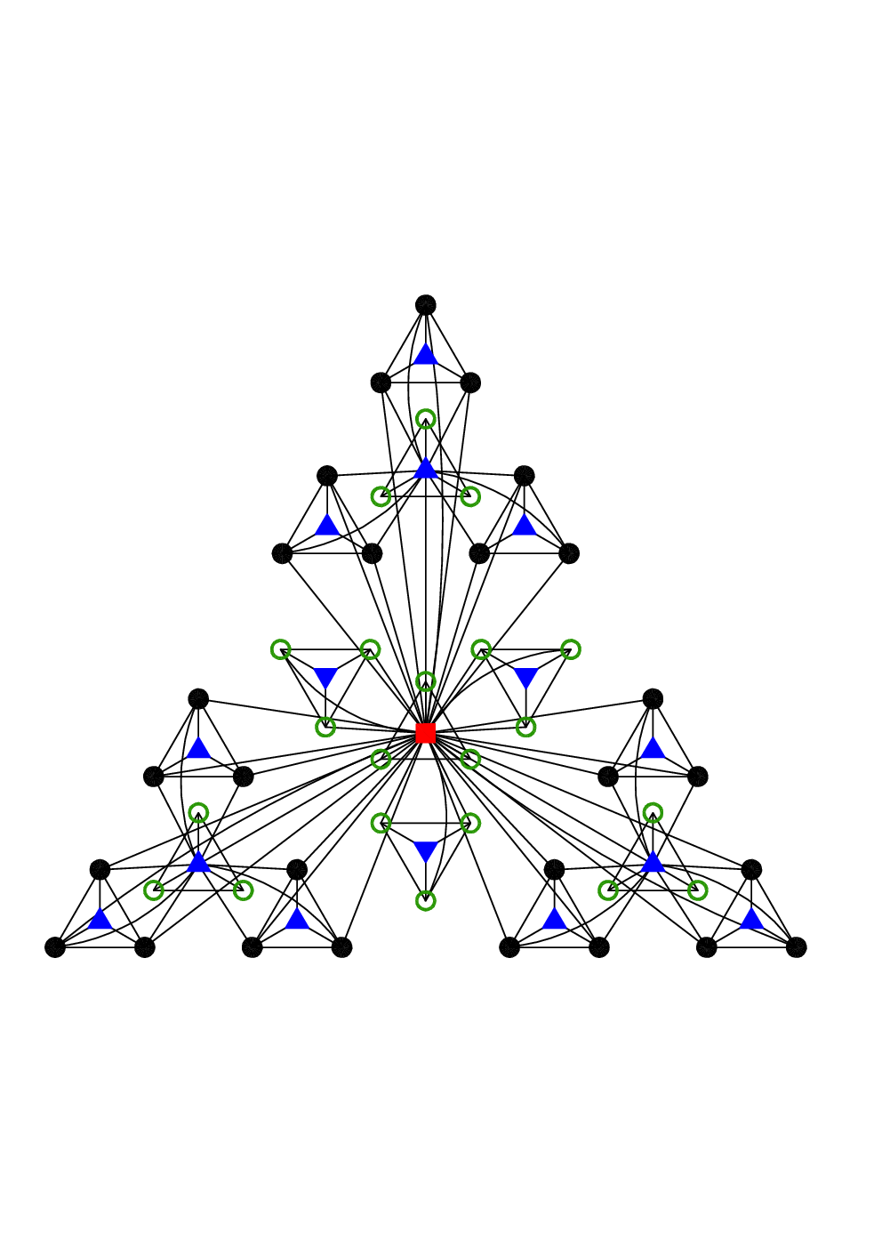
The hierarchical networks present some typical properties of real systems in nature and society [65]. They are scale free with the degree distribution exponent . The average path length, defined as the shortest distance averaged over all pairs of nodes, scales logarithmically with the number of nodes. In the large network order limit, the average clustering coefficient tends to a large constant dependent on . Thus, the whole family of networks exhibits small-world behavior [67]. In addition, the betweenness of nodes in the networks follows the same power-law distribution irrespective of . In particular, the networks show an obvious modular structure. All these characteristics are not shared by other models. The peculiar topological features make the networks unique within the category of scale-free networks; it therefore is worthwhile to investigate various dynamical processes running on them. In what follows we will study the trapping problem on this class of modular networks to uncover the influence of the particular topologies on the trapping process.
III Formulation of the trapping problem
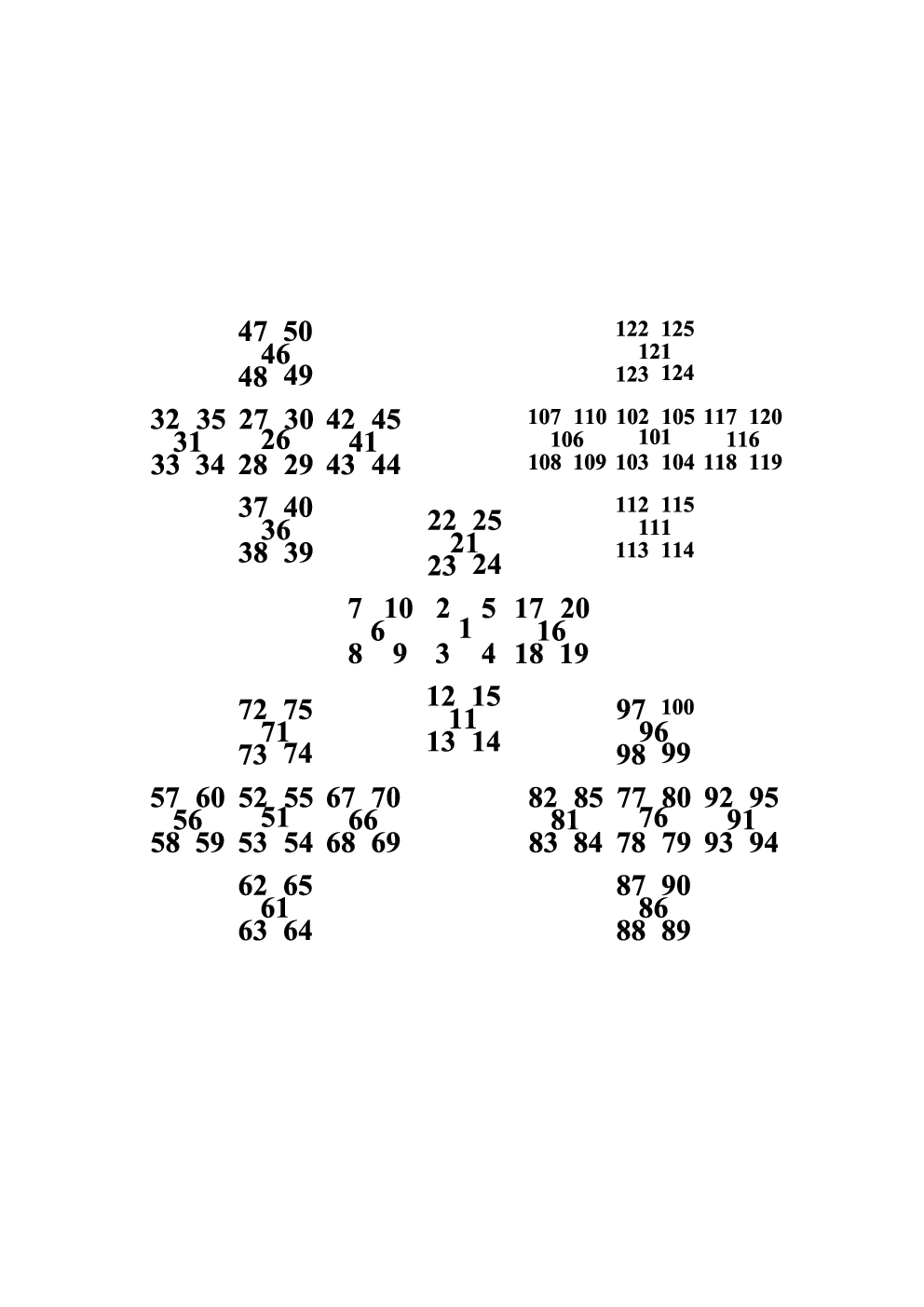
In this section we formulate the trapping problem on the family of hierarchical scale-free networks , which is actually a simple unbiased Markovian random walk of a particle in the presence of a trap or a perfect absorber located on a given node. To facilitate the description, we distinguish different nodes in by assigning each of them a labeling in the following way. The hub node in has label 1; the other peripheral nodes in are labeled as 2, 3, and , respectively. Assume that we have labeled nodes in consecutively by 1, 2, and ; in the next generation , we keep the labels of nodes in the original unchanged and label only the nodes belonging to the copies of by assigning to each node a different integer from to . In this way, every node in is labeled by a unique integer from 1 to ; see Fig. 3.
For convenience, we continue to represent by its adjacency matrix of order , whose element is defined as follows: if and are neighboring nodes and otherwise. Then the degree, , of node is given by , the diagonal degree matrix of is , and the normalized Laplacian matrix of is provided by , where is the identity matrix.
Before proceeding further, let us introduce the so-called discrete-time random walk on . At each time step, the particle jumps from its current location to any of its nearest neighbors with equal probability. According to this rule, at time , a particle located at a node will hop to one of its neighbors, say , with the transition probability . Suppose that the particle starts off from node at , then the jumping probability of going from to at time is governed by the following master equation [22]:
| (11) |
We next focus the trapping problem on with the trap fixed on the hub node, i.e., node 1, represented as . The particular choice for the trap position allows to compute analytically the MFPT, which will be discussed in detail in the following section. Similar to the standard discrete-time random walks, during the trapping process, in a single time step, the particle, starting from any node except the trap , jumps to any of its nearest neighbors with the same probability. What we are concerned with is the expected time that the particle spends, starting from a source node before being trapped, which is in fact a random variable. Let be the expected time, frequently called first-passage time (FPT) or trapping time, for a walker, starting from node , to first arrive at the trap . In order to determine , we define to be the probability for the particle, starting from point , to first hit the trap after steps. Notice that since the Markov chain [68] representing such a random walk is ergodic, the particle will be eventually trapped independently of the origin, implying that holds for all . It is easily known that the set of these interesting quantities obeys the following recurrence relation:
| (12) |
where .
Let be the corresponding generating function of quantity :
| (13) |
which encapsulates all the information contained in the discrete probability distribution . For example, the expected value is the first derivative of evaluated at .
Let stand for the -dimensional vector , where the superscript represents the transpose of the vector. According to Eqs. (12) and (13), we have
| (14) |
where is a matrix with order with entry . Differentiating the two sides of Eq. (14) with respect to and doing some simple algebra operations, we have
| (15) |
in which is the identity matrix with order ; is the -dimensional zero vector . Setting in Eq. (15) leads to
| (16) |
where is the -dimensional unit vector. Actually, in Eq. (16) is the fundamental matrix of the Markov chain representing the unbiased random walk, and is a submatrix of the normalized discrete Laplacian matrix of , which is obtained from by removing from the first row and column corresponding to the trap.
From Eq. (16), the mean first-passage time, , which is the average of over all initial nodes distributed uniformly over nodes in other than the trap, is given by
| (17) |
where is the corresponding element of matrix , which is the mean time that the particle spends at node starting from node [69].
Equation (17) shows that the problem of calculating MFPT is reduced to finding the sum of all elements of matrix . Since the order of is , where increases exponentially with , for large , inverting matrix is prohibitively time and memory consuming, making it intractable to obtain through direct calculation from Eq. (17); one can compute directly the MFPT only for the first several generations (see Fig. 4). Hence, an alternative method of computing MFPT becomes necessary. In [70], to allow for a drastic reduction in computational cost, a scheme was proposed mapping the original Markov process on another Markov process. Although the method can bring down the computational efforts, it is an approximate one. Fortunately, the special recursive construction of the hierarchical networks allows to calculate analytically MFPT to obtain an explicit solution for arbitrary generation . In the next section, we will provide the detailed process for the derivation of MFPT using a method significantly different from that applied in [41, 42, 43, 45].

IV Closed-form solution to mean first-passage time
Prior to deriving the general formula for MFPT, , for the trapping issue on , we first define some related quantities. Let denote the probability that, at the generation , the particle starting from any peripheral node in first arrives at the hub after jumps; and let represent the probability that, the walker originating from the hub to first reach any node belonging to after steps. Then, the following fundamental relations can be established:
| (18) | |||||
and
| (19) |
where is the Kronecker delta function that is defined as follows: if is equal to 1, and otherwise. Note that in Eqs. (18) and (19), the equivalence of nodes in the same set (e.g., or ) was used.
The three terms on the right-hand side (rhs) of Eq. (18) can be elaborated as follows: the first term accounts for the probability that the walker takes only one time step to first reach the hub; the second term on the rhs explains the case that the particle gets first to one of its neighbors belonging to in one time step, and then it takes more steps to first arrive at the target node; the last term on the rhs describes the probability of the process in which the walker first makes a jump to a local hub node belonging to , then it takes time steps, starting from the local hub, to hit one of the nodes in , and continues to jump more steps to first reach the hub.
Analogously, the two terms on the rhs of Eq. (19) can be understood based on the following two processes. The first term explains the occurring probability of the process that the walker, starting from the hub, only needs one time step to reach a peripheral node in . The second term represents the happening probability of such a process that the particle, originating from the hub, first makes one jump to a local peripheral node in , then makes jumps to the hub, and proceeds to the destination (one of the nodes in ), taking more time steps.
Equations (18) and (19) provide the two basic relations governing the trapping problem performing on , from which almost all subsequent results are derived from. As shown in the preceding section, although we are concerned about only the fundamental quantity (namely, MFPT), the direct calculations are practically hard and intractable for large networks. Nevertheless, the particular construction of the networks allows to overcome this difficulty in virtue of the powerful mathematical technique of generating functions [64], through which we can compute and determine the MFPT indirectly.
First, we define two generating functions, and , for the probability distribution of first-passage time described in Eqs. (18) and (19), which can be written as
and
After some algebraic operations, Eqs. (IV) and (IV) can be recast, respectively, as
| (22) |
and
| (23) |
Let denote the first-passage time for a walker starting from an arbitrary node in to reach the hub for the first time, which is in fact the number of steps for the walker originating from any node in to first visit the hub. Let stand for the FPT needed for a particle initially located at the hub to first hit any node in . Then, according to the property of generating functions, the two quantities and are given separately by
| (24) |
and
| (25) |
Differentiating, respectively, both sides of Eqs. (22) and (23) with respect to and setting , we obtain the following two coupled relations:
| (26) |
and
| (27) |
From the above two coupled equations, it is not difficult to have
| (28) |
and
| (29) |
Considering the initial conditions and , we can solve the simultaneous equations, i.e., Eqs. (28) and (29), to obtain
| (30) |
and
| (31) |
The obtained expressions for and are very important, using which we will determine MFPT . To facilitate the computation, we use to represent the set of nodes in and separate them into two subsets: one subset is made up of nodes in the original , and the other subset, denoted by , is the set of nodes of the copies of . Let denote the trapping time for a walker originating at node on the th generation network to first reach the trap node (hub). Obviously, for all , . For , it is a trivial case, we have . Then, by definition, the MFPT can be expressed as
| (32) |
where the sum term can be rewritten as
| (33) | |||||
which is obvious from the particular construction of the hierarchical networks. Thus, we have
| (34) |
Hence, to obtain an exact solution for , all that is left is to evaluate the sum in Eq. (34), with a goal to first find a recursive relation for . From Figs. 1 and 2, the sum term on the rhs of Eq. (34) can be evaluated as follows:
| (35) |
Substituting previously obtained equations for the expressions of related quantities in Eq. (35) and combining with Eq. (33), we can obtain the following recurrence relation for :
| (36) | |||||
Using the initial condition , Eq. (36) is solved inductively to obtain the rigorous expression for the MFPT:
| (37) | |||||
We have checked our analytic formula against numerical values obtained according to the fundamental matrix provided by Eq. (17). For different parameters and , the values obtained from Eq. (37) completely agree with those numerical results on the basis of the direct calculation through Eq. (17); see Fig. 4. This agreement serves as an independent test of our theoretical formula. Moreover, we have performed genuine simulations of the random walk process on the hierarchical networks. The data from the true process are shown in Fig. 4, each of which is obtained by averaging over realizations. The results of the true simulations are in excellent agreement with our analytical ones given by Eq. (37), and thus provide an important further evidence in favor of our findings.
We continue to show how to represent MFPT in terms of network order with the aim to obtain the scaling between these two quantities. Recalling , we have . Hence, Eq. (37) can be rewritten as
| (38) | |||||
Thus, for networks with large order, i.e., ,
| (39) |
where the exponent is lower than 1. Clearly, is a decreasing function of : when grows from 3 to infinite, descends from and approaches to zero, which means that the efficiency of the trapping process depends on . The larger the value of , the more efficient the trapping process. Equation (39) also implies that in the infinite network order limit, the MFPT grows algebraically with increasing order of the networks.
The above obtained scaling of MFPT with order of the hierarchical scale-free networks is quite different from those scalings for other media. For instance, on regular lattices with large order , the asymptotical behavior of MFPT is , , and for dimensions , , and , respectively [36]. Again for example, on planar Sierpinski gasket [37] and Sierpinski tower [38] in three Euclidean dimensions, and the fractal [39], the MFPT scales superlinearly with network order; i.e., it grows as a power-law function of network order with the exponents being 1.464, 1.293, and 1.631, respectively. Finally, for the pseudofractal web [41], the Koch network [42], and the Apollonian network [43], they are all scale free, their MFPT scales linearly or sublinearly with network order, following separately the asymptotical behaviors , , and . Thus, compared with the aforementioned regular networks, fractals, even scale-free networks, the addressed hierarchical networks exhibit more efficient configuration for random walks with a single trap fixed at the node with highest degree.
The root of the high efficiency of the trapping problem on the hierarchical scale-free networks lies in their architecture. In this network family, there are many small densely interconnected clusters, which combine to form larger but less compact groups connected by nodes with high degrees (i.e., local hub nodes). The relatively large groups are further joined to shape even larger and even less densely interlinked modules. These modules or groups are combined again at a “large” node forming a fine hierarchical structure that is responsible for the fast diffusion phenomenon, which can be understood from the following heuristic argument. When a walker starts off from some node, it will either hit the hub directly or first get to local hub nodes. These local hubs, although not connected to the trap node, play the role of bridges linking different modules together at the local peripheral nodes, through which the walker may easily find the way to the trap. Thus, the walker can visit the trap in a short time, disregarding its starting points.
V Conclusions
In conclusion, we have investigated the classic trapping problem on a class of hierarchical networks that can bring under a single roof the scale-free and modular topologies, which are two striking structural properties observed in various biological and social networks. Thus, the hierarchical networks can mimic some real-world natural and social systems to some extent (to what extent it does is still an open question). Using the method of generating functions, we derived the recursion relations governing the evolution of the MFPT for random walks on the networks, with the only trap located at the hub node. These recursive relations are obtained from the special construction of the networks, from which we determined explicitly the solution for the MFPT, which shows that the MFPT varies algebraically with network order as with the exponent much less than 1 that decreases from to zero when increases from 3 to infinite. Thus, in the full range of , the efficiency of the trapping process on the hierarchical networks is high. We have also compared the result with those previously obtained for other media, and found that in marked contrast to other graphs, the hierarchical networks have more efficient structure that tends to speed up the diffusion process. Finally, it deserves to be mentioned that although the hierarchical networks are efficient for the trapping problem with the trap fixed on the hub, they might lose this characteristic when the trap is positioned at a randomly selected node, due to the somewhat tree-like macro-structure of this kind of networks [28, 66].
Acknowledgment
We would like to thank Xing Li for support. This research was supported by the National Natural Science Foundation of China under Grants No. 60704044, No. 60873040, and No. 60873070, the National Basic Research Program of China under Grant No. 2007CB310806, Shanghai Leading Academic Discipline Project No. B114, and the Program for New Century Excellent Talents in University of China (Grants No. NCET-06-0376). S. Y. G. also acknowledges the support by Fudan’s Undergraduate Research Opportunities Program.
References
- [1] R. Albert and A.-L. Barabási, Rev. Mod. Phys. 74, 47 (2002).
- [2] S. N. Dorogovtsev and J. F. F. Mendes, Adv. Phys. 51, 1079 (2002).
- [3] M. E. J. Newman, SIAM Rev. 45, 167 (2003).
- [4] S. Boccaletti, V. Latora, Y. Moreno, M. Chavez and D.-U. Hwanga, Phys. Rep. 424, 175 (2006).
- [5] A.-L. Barabási and R. Albert, Science 286, 509 (1999).
- [6] M. Girvan and M. E. J. Newman, Proc. Natl. Acad. Sci. U.S.A. 99, 7821 (2002).
- [7] E. Ravasz, A. L. Somera, D. A. Mongru. Z. N. Oltvai, and A.-L. Barabási, Science 297, 1551 (2002).
- [8] E. Ravasz and A.-L. Barabási, Phys. Rev. E 67, 026112 (2003).
- [9] L. Danon, J. Duch, A. Diaz-Guilera, and A. Arenas, J. Stat. Mech.: Theory Exp. (2005) P09008.
- [10] G. Palla, I. Derényi, I. Farkas, and T. Vicsek, Nature (London) 435, 814 (2005).
- [11] M. E. J. Newman, Proc. Natl. Acad. Sci. U.S.A. 103, 8577 (2006).
- [12] S. Fortunato, e-print arXiv:0906.0612.
- [13] F. Chung and L. Lu, Proc. Natl. Acad. Sci. U.S.A. 99, 15879 (2002).
- [14] R. Cohen and S. Havlin, Phys. Rev. Lett. 90, 058701 (2003).
- [15] S. N. Dorogovtsev, A. V. Goltsev and J.F.F. Mendes, Rev. Mod. Phys. 80, 1275 (2008).
- [16] S. Havlin and D. ben-Avraham, Adv. Phys. 36, 695 (1987).
- [17] R. Metzler and J. Klafter, Phys. Rep. 339, 1 (2000).
- [18] R. Metzler and J. Klafter, J. Phys. A 37, R161 (2004).
- [19] R Burioni and D Cassi, J. Phys. A 38, R45 (2005).
- [20] I. M. Sokolov, J. Mai, and A. Blumen, Phys. Rev. Lett. 79, 857 (1997).
- [21] S. A. Pandit and R. E. Amritkar, Phys. Rev. E 63, 041104 (2001).
- [22] J. D. Noh and H. Rieger, Phys. Rev. Lett. 92, 118701 (2004).
- [23] O. Bénichou, M. Coppey, M. Moreau, P.-H. Suet, and R. Voituriez, Phys. Rev. Lett. 94, 198101 (2005).
- [24] V. Sood, S. Redner, and D. ben-Avraham, J. Phys. A: Math. Gen. 38, 109 (2005).
- [25] E. M. Bollt, D. ben-Avraham, New J. Phys. 7, 26 (2005).
- [26] L. K. Gallos, C. Song, S. Havlin, and H. A. Makse, Proc. Natl. Acad. Sci. U.S.A. 104, 7746 (2007).
- [27] P. Barthelemy, J. Bertolotti, and D. S. Wiersma, Nature (London) 453, 495 (2008). .
- [28] A. Baronchelli, M. Catanzaro, and R. Pastor-Satorras, Phys. Rev. E 78, 011114 (2008).
- [29] A. Kittas, S. Carmi, S. Havlin, and P. Argyrakis, EPL 84, 40008 (2008).
- [30] Z. Z. Zhang, Y. C. Zhang, S. G. Zhou, M. Yin, and J. H. Guan, J. Math. Phys. 50, 033514 (2009).
- [31] C. P. Haynes and A. P. Roberts, Phys. Rev. Lett. 103, 020601 (2009).
- [32] F. Jasch and A. Blumen, Phys. Rev. E 63, 041108 (2001).
- [33] M. F. Shlesinger, Nature (London) 443, 281 (2006).
- [34] J. Whitmarsh and J. A. Govindjee, in Concepts in Photobiology: Photosynthesis and Photomorphogenesis, edited by G. Singhal, G. Renger, S. Sopory, K.-D. Irrgang, and J. A. Govindjee (Narosa, New Delhi, 1999), pp. 11-51.
- [35] F. Fouss, A. Pirotte, J. M. Renders, and M. Saerens, IEEE Trans. Knowl. Data Eng. 19, 355 (2007).
- [36] E. W. Montroll, J. Math. Phys. 10, 753 (1969).
- [37] J. J. Kozak and V. Balakrishnan, Phys. Rev. E 65, 021105 (2002).
- [38] J. J. Kozak and V. Balakrishnan, Int. J. Bifurcation Chaos Appl. Sci. Eng. 12, 2379 (2002).
- [39] E. Agliari, Phys. Rev. E 77, 011128 (2008).
- [40] A. Garcia Cantú and E. Abad, Phys. Rev. E 77, 031121 (2008).
- [41] Z. Z. Zhang, Y. Qi, S. G. Zhou, W. L. Xie, and J. H. Guan, Phys. Rev. E 79, 021127 (2009).
- [42] Z. Z. Zhang, S. G. Zhou, W. L. Xie, L. C. Chen, Y. Lin, and J. H. Guan, Phys. Rev. E 79, 061113 (2009).
- [43] Z. Z. Zhang, J. H. Guan, W. L. Xie, Y. Qi, and S. G. Zhou, EPL, 86, 10006 (2009).
- [44] E. Agliari and R. Burioni, Phys. Rev. E 80, 031125 (2009).
- [45] Z. Z. Zhang, W. L. Xie, S. G. Zhou, S. Y. Gao, and J. H. Guan, EPL 88, 10001 (2009).
- [46] S. Condamin, O. Bénichou, V. Tejedor, R. Voituriez, and J. Klafter, Nature (London) 450, 77 (2007).
- [47] O. Bénichou, B. Meyer, V. Tejedor, and R. Voituriez, Phys. Rev. Lett. 101, 130601 (2008).
- [48] S. Condamin, V. Tejedor, R. Voituriez, O. Bénichou and J. Klafter, Proc. Natl. Acad. Sci. U.S.A. 105, 5675 (2008).
- [49] R. Guimerà, M. Sales-Padro and L. A. N. Amaral, Nat. Phys. 3, 63 (2007).
- [50] S. Maslov, Nat. Phys. 3, 18 (2007).
- [51] A.-L. Barabási, E. Ravasz, and T. Vicsek, Physica A 299, 559 (2001).
- [52] S. N. Dorogovtsev, A. V. Goltsev, and J. F. F. Mendes, Phys. Rev. E 65, 066122 (2002).
- [53] S. Jung, S. Kim, and B. Kahng, Phys. Rev. E 65, 056101 (2002).
- [54] F. Comellas, J. Ozón, and J.G. Peters, Inf. Process. Lett. 76, 83 (2000)
- [55] Z. Z. Zhang, L. L Rong, and C. H. Guo, Physica A 363, 567 (2006).
- [56] M. Hinczewski and A. N. Berker, Phys. Rev. E 73, 066126 (2006).
- [57] H. D. Rozenfeld, S. Havlin, and D. ben-Avraham, New J. Phys. 9, 175 (2007).
- [58] M. Hinczewski, Phys. Rev. E 75, 061104 (2007).
- [59] Z. Z. Zhang, S. G. Zhou, T. Zou, L. C. Chen, and J. H. Guan, Eur. Phys. J. B 60, 259 (2007).
- [60] Z. Z. Zhang, S. G. Zhou, L. J. Fang, J. H. Guan, and Y. C. Zhang, EPL 79, 38007 (2007).
- [61] F. Comellas and A. Miralles, Physica A. 388, 2227 (2009).
- [62] G. H. Weiss, Aspects and Applications of the Random Walk (North Holland, Amsterdam, 1994).
- [63] S. Redner, A Guide to First-Passage Processes (Cambridge University Press, Cambridge, 2001).
- [64] H. S. Wilf, Generatingfunctionology, 2nd ed. (Academic Press, London, 1994).
- [65] J. D. Noh, Phys. Rev. E 67, 045103(R) (2003).
- [66] J. D. Noh and H. Rieger, Phys. Rev. E 69, 036111 (2004).
- [67] D. J. Watts and H. Strogatz, Nature (London) 393, 440 (1998).
- [68] J. G. Kemeny and J. L. Snell, Finite Markov Chains (Springer, New York, 1976).
- [69] A. Bar-Haim and J. Klafter, J. Chem. Phys. 109, 5187 (1998).
- [70] A. Baronchelli and V. Loreto, Phys. Rev. E 73, 026103 (2006).