Density-matrix-renormalization-group study of excitons
in
poly-diacetylene chains
Abstract
We study the elementary excitations of a model Hamiltonian for the -electrons in poly-diacetylene chains. In these materials, the bare band gap is only half the size of the observed single-particle gap and the binding energy of the exciton of 0.5 eV amounts to 20% of the single-particle gap. Therefore, exchange and correlations due to the long-range Coulomb interaction require a numerically exact treatment which we carry out using the density-matrix renormalization group (DMRG) method. Employing both the Hubbard–Ohno potential and the screened potential in one dimension, we reproduce the experimental results for the binding energy of the singlet exciton and its polarizability. Our results indicate that there are optically dark states below the singlet exciton, in agreement with experiment. In addition, we find a weakly bound second exciton with a binding energy of 0.1 eV. The energies in the triplet sector do not match the experimental data quantitatively, probably because we do not include polaronic relaxation effects.
pacs
71.20.Rv, 71.10.Fd, 78.30.Jw, 78.20.BhI Introduction
I.1 Experimental observations
I.1.1 Structure
Poly-diacetylenes (PDAs) are prototypical quasi one-dimensional materials. [1, 2] Their monomer building unit is comprised of four carbon atoms. The four outer electrons of each carbon atom are sp2 hybridized. Three of them form -bonds. The -bonds are between neighboring carbon atoms on the chain and to covalent ligands and , which are several Å long and differ for various members of the PDA family. The fourth electron is delocalized over the carbon backbone in a molecular -orbital.

The resulting Lewis structure is shown in Fig. 1. The four carbon atoms in the unit cell are linked by a triple bond, a single bond, a double bond, and a single bond. The atomic distances are , , and for the single (S), double (D), and triple bonds (T), respectively. The chain of atoms is not perfectly straight; the single and double bonds alternately form angles of and degrees.
Very long undistorted polymer chains have been built starting from a monomer single crystal so that the chains are perfectly ordered, [1] and single polymer chains diluted in their monomer matrix have even been prepared and studied. [3] In PDAs, exciton-polaritons have been generated that have been shown to be coherent over tens of micrometers, i.e., several ten thousand monomer units. [4] Consequently, the opto-electronic properties of the PDAs result from the electrons’ mutual interaction and their interaction with the periodic lattice potential, while the influence of disorder is negligible.
I.1.2 Optical properties
PDAs are insulators; the gap for single-particle excitation is . Band structure calculations estimate the bare band gap to be , i.e., electronic exchange and correlations account for half of the single-particle gap. Moreover, the optical gap for the primary exciton is , so that the exciton binding energy is about 20% of the band gap. Due to the restricted geometry, the electron-electron interaction must be treated accurately for the calculation of the optical properties of the PDAs.
Lattice effects complicate the analysis of the spectra of PDAs in two ways. First, the primary exciton with excitation energy is accompanied by phonon sidebands that result from oscillations of the double and triple bonds. These signals dominate the optical excitations below the band gap. Second, some PDA single crystals such as TCDU [5] exist in two different conformations, which have exciton energies (‘blue chains’) and (‘red chains’), respectively. Therefore, it is not easy to disentangle the effects of the electron-electron interaction from those of the electron-lattice interaction; the latter gives rise to resonance shifts of several tenths of an electron volt.
I.2 Theoretical approaches
I.2.1 Extended Wannier theory
In order to describe the optical excitations in PDAs, two approaches have been taken. The first approach starts from an ab-initio density-functional theory calculation of the bare band structure in local-density approximation (LDA), which is then supplemented by an approximate treatment of the residual electron-electron interaction, e.g., the approximation for the single-particle bands and the Bethe-Salpeter equation (BSE) for the excitons (LDA++BSE). [6, 7] Actual calculations for the PDAs often omit the step (Wannier theory). [8] Within this approach, a number of experimental data could be reproduced, e.g., the exciton binding energy and its polarizability. Unfortunately, the theory does not predict optically dark states below the exciton resonance.
I.2.2 Model calculations
The second approach to a theoretical description of the primary excitations in polymers starts from a many-particle model Hamiltonian that describes only the -electrons and their mutual interaction. The parameters for the kinetic energy of the electrons are taken from LDA calculations, and the Coulomb interaction is approximated in various ways, e.g., with the Ohno parametrization [9] of the Pariser–Parr–Pople potential. [10] With the help of the DMRG method, [11] the ground state and elementary excitations for such models can be calculated for large chains with a very high accuracy. In this way, the electron-electron interaction is treated without resorting to any approximations. Unfortunately, specific calculations for the PDAs [12] have only had limited success in meeting the experimental test.
I.2.3 Simplifying assumptions and outline of this work
In this work, we consider structures which start with a triple bond and end with a double bond, i.e., we consider the sequences [(TSDS)m-1TSD] of carbon atoms with triple bonds and double bonds. We perform a DMRG study of a many-body model Hamiltonian for the -electrons which uses Barford and Bursill’s parametrization for the band-structure part [12] but employs the screened Coulomb potential in one dimension. The essential difference between the screened potential and the Ohno potential is that the local interaction part is larger in the screened potential. Because of this, the Hubbard–Ohno potential leads to a good description of the low-energy singlet excitations in PDAs.
We do not include lattice relaxation for the single-particle and optical excitations. As has been shown by Barford and co-workers, [13] the relaxation energies for triplet excitons in trans-polyacetylene can be as large as . The parameter sets we will use below apply to the rigid-lattice situation and will change slightly when lattice relaxation is taken into account properly.
The different varieties of PDA differ in their ligands, which introduce local potentials on the carbon atoms with double bonds. Therefore, the excitation energies of the PDAs differ by a few tenths of an electron volt. In this work, we ignore the ligand effects and only consider a prototypical case.
II Model for poly-diacetylene
II.1 Operators in second quantization
II.1.1 Kinetic energy operator, current operator, and dipole operator
In this work we will restrict ourselves to the description of the electrons because they dominate the optical response of the poly-diacetylenes for energies . The motion of the electrons is described by the operator for the kinetic energy,
| (1) |
where , are creation and annihilation operators, respectively, for electrons with spin on site with three-dimensional coordinate . The matrix elements are the electron transfer amplitudes between neighboring sites. Following Ref. 12 we set
| (2) |
for the single, double, and triple bonds, respectively. We consider the half-filled band exclusively, i.e., the number of electrons equals the number of lattice sites .
The electrical current operator is given by
| (3) |
where is an average bond length, i.e., we ignore geometry effects in due to the difference in bond lengths.[14]
Finally, we define the operator for the dipole moment,
| (4) |
Here counts the number of electrons on site , and is the local density operator at site for spin . Recall that we treat the PDA chain as perfectly straight, so that is the appropriate sum over the bond distances , , and for the single, double, and triplet bonds between the sites and .
II.1.2 Coulomb interaction
The electrons interact electrostatically via the Coulomb interaction (Pariser–Parr–Pople model [10])
| (5) | |||||
The PDAs are insulators. Therefore, the Coulomb interaction is not dynamically screened at the energy scale of a few electron volts, and the screening is taken into account reasonably well by a static dielectric screening with dielectric constant for PDAs.
For the description of electrons and holes in quantum wires and other quasi one-dimensional structures, various effective potentials have been used in the literature. [15, 16] For polymers, the general Pariser–Parr–Pople potential [10] is often approximated by the semi-empirical Ohno potential, [9, 12, 17]
| (6) |
with . At large distances, the Coulomb interaction must be recovered. Therefore, we require
| (7) |
which implies , where we have used that is the Rydberg energy and is the Bohr radius. The remaining free parameter describes the modification of the Coulomb potential at short distances due to the confinement of the electrons to the chain. Below, we derive the Ohno potential and justify it for intermediate to large length scales. For short distances, however, the Hubbard interaction must be kept explicitly, leading to an additional parameter.
II.1.3 Effective Coulomb potentials
Our derivation of the one-dimensional effective potentials for the various cases closely follows Refs. 18 and 19. In order to set up the single-particle basis in which the one-dimensional Hamiltonian (5) is formulated, we solve the single-particle Schrödinger equation for electrons whose motion is restricted to the -direction due to a confining potential. We set , so that the single-particle wave functions factorize: . The potential incorporates the (small) effects of the various ligands and permits a discrimination of the poly-diacetylenes. For the purpose of this work, we set it to a constant which we absorb into .
The confining potential perpendicular to the chain direction is assumed to be very strong so that the electron wave function in the direction perpendicular to the chain is given by the lowest-energy state . The effective Coulomb potential between two charges at distance is then given by [18, 19]
| (8) |
This expression can be simplified further for a parabolic confining potential, [19]
| (9) |
where the parameter characterizes the strength of the confining potential. The ground-state wave function of the harmonic oscillators in the and directions is given by
| (10) |
where is a Gaussian with standard deviation . This means that we find the electrons in the region with a probability of more than 90 percent. In poly-diacetylene single crystals, [20] the distance between chains is typically so that the condition of weak overlap between the chains, , is fulfilled for . This view is supported by the fact that the optical excitations for poly-diacetylene single crystals do not differ much from those for single chains diluted in their single-crystal monomer matrix. [21] The excitation energy to the next confinement level is . For , the excitation energy to the next confinement level is so that higher confinement levels are not thermally populated at room temperature.
When we insert (10) into (8), we can carry out the Gaussian integrals in the coordinates and and are left with a double integral over and . In polar coordinates, the resulting angular integral becomes trivial and we find [19]
| (11) | |||||
where is the error function.
We compare the long-distance limit of (11) with that of the Ohno potential (6). We demand the coefficients of the order and agree and, with the help of Eq. (7.1.23) in Ref. 22, find that
| (12) |
or , with the unit of length. In terms of the confinement parameter , the screened potential and the Ohno potential can be cast into the form
| (13) | |||||
| (14) |
whose large-distance expansions differ only to order . A comparison of the screened potential and the Ohno potential for all distances is shown in Fig. 2. The agreement is to better than 10% for all . Even at , the discrepancy is only 25%. Therefore, it is justified to replace the screened potential by the Ohno potential for intermediate distances. At short distances, the differences between the Ohno potential and the screened potential are substantial. The Ohno potential at is , in contrast to with .
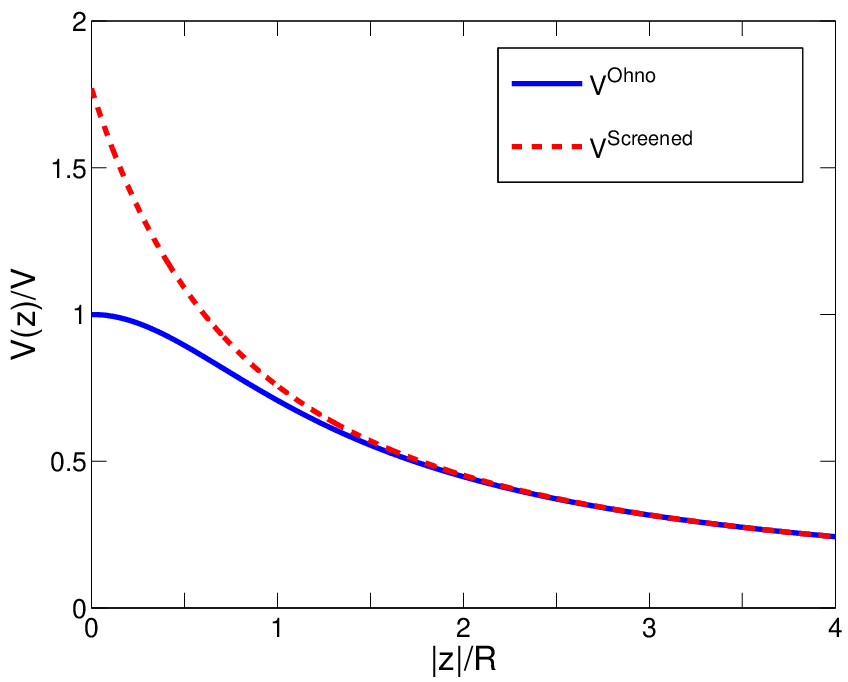
The above derivation applies to a straight geometry, not to the zigzag geometry of the Lewis structure in poly-diacetylenes. We account for the corresponding reduction of the chain length by the approximation as in the Ohno potential (6), thereby ignoring the minor changes due to the non-orthogonality of the chain axis and the -axis.
II.2 Hamilton operator
II.2.1 Hubbard–Ohno potential and screened potential
In this work, we study the correlated motion of electrons along a chain, which we model using the Hamiltonian
| (15) |
We use the Hubbard–Ohno potential
| (16) |
for and . Here the effective Coulomb parameter is linked to the screening length via Eq. (12), . For example, we find for . The Hubbard–Ohno potential was used earlier by Chandross, Mazumdar et al. [23] to explain the main absorption features of poly(para-phenylene vinylene) (PPV) with the parameter set and . Our derivation in Sect. II.1.3 justifies their modification of the Ohno potential, and their results for PPV support our choice for .
For comparison, we also give results for the screened potential,
| (17) | |||||
which implies . Again, we have . For example, we find for .
II.2.2 Particle-hole symmetry
The Hamiltonian (15) and the current operator (3) are invariant under the particle-hole transformation . At half band-filling, the ground state is also invariant under this transformation. Therefore, the expectation value of the dipole operator (4) vanishes in the ground state, . Likewise, the expectation values of the current operator vanishes in the ground state, .
We expect the same relation for excitons (bound particle-hole excitations of the ground state at half band-filling). Therefore, in the presence of a weak electrical field, such states show a quadratic Stark effect, see Sect. III.2.
III Method
III.1 Single-particle gap and exciton binding energy
Our model description contains a single parameter that can be taken to be the screening length or the Coulomb parameter . We use this parameter to adjust the typical band gap in poly-diacetylenes. The band gap or single-particle gap is defined by the difference in chemical potentials for a system with and particles,
| (18) | |||||
which, due to particle-hole symmetry at half band-filling, reduces to
| (19) |
where is the energy of the -particle ground state . Optical excitations to above the single-particle gap are extended and thus can transport current through the system. Experimentally, they can be monitored by the onset of the Franz–Keldysh oscillations in the electro-absorption signal. Typical values for poly-diacetylene single crystals are for DCHD and for PTS and PFBS. [20]
In poly-diacetylenes, the singlet exciton and its vibronic replicas carry most of the oscillator strength of the optical excitations. The quadratic Stark effect in the electro-absorption proves that they are bound states of electron-hole excitations. [20] The exciton energy thus defines the optical gap,
| (20) |
where is the energy of the first excited state of the half-filled system , which has a finite overlap with an optical excitation of the ground state, . The binding energy of the excitons is then obtained as
| (21) |
For DCHD and PTS/PFBS PDA single crystals, the corresponding binding energies are and , respectively. [20]
In our numerical investigation, we calculate the ground state and excited states , . An optical excitation with the current operator , Eq. (3), has the oscillator strength
| (22) |
Amongst the excited states , we identify the exciton state as the energetically lowest-lying excitation that carries significant optical weight, . The same description can be obtained using the dipole operator given by Eq. (4).
III.2 Polarizability and exciton wave function
Since it is a bound state, the exciton displays a quadratic Stark effect, i.e., the redshift of the resonance level with an external static electrical field of strength is given by
| (23) |
where is the polarizability. Note that the experiment measures the Stark shift both of the ground state and of the exciton . In our calculations, we determine and for various fields from the Hamiltonian
| (24) |
with the dipole operator , see Eq. (4). Note that we determine the polarizability as measured in experiment, i.e., we need not resort to further theoretical considerations here.
In order to extract the ‘exciton radius’ from the polarizability, one can start from the Frenkel picture [24] or from the Wannier picture. [20] As demonstrated in Ref. 25, the probability distribution provides a very detailed picture of the spatial character of the exciton in a many-particle approach. It describes the particle-hole content of the exciton wave function with respect to the ground state, i.e., it gives the probability that is an electron-hole excitation of the ground state at sites and , respectively. Explicitly,
| (25) | |||||
|
and |
|||||
| (26) | |||||
We denote the probability density to find an electron-hole pair at a separation by ,
| (27) |
The average electron-hole distance is then obtained from
| (28) |
In Ref. 20, a simple two-level model was considered in which the exciton couples to a (representative) continuum state. As we shall see in Sect. IV.4, the two corresponding electron-hole distances compare well with each other.
III.3 Numerical procedure
We present results both for the Hubbard–Ohno potential, Eq. (16), and for the screened potential, Eq. (17). In the presence of long-ranged Coulomb interactions, a high numerical accuracy is of crucial importance. Therefore, we devote this subsection to the problem of how we determine and control the accuracy of our calculations.
In this work, we have performed the numerical calculations on finite chains with open boundary condition (OBC) using the non-local version [26, 27, 28] of the DMRG technique.[29] The number of block states has been selected according to the dynamic block-state selection (DBSS) approach.[28, 30]
III.3.1 Ground state and single-particle gaps
In order to calculate the band and spin gaps, we have determined the lowest-lying eigenstates of various spin and charge sectors from independent DMRG runs. In this case, the DBSS approach [28, 30] permits a rigorous control of the numerical accuracy because we can fix the threshold value of the quantum information loss . Here we take . As another check, we have used the entropy sum rule for finite chain lengths for each DMRG sweep, i.e., we have verified that the sum rule has been satisfied after the third sweep. During our calculations, the maximum number of block states was varied in the range for OBC due to the large spin and band gaps. For , the maximal chain length is . For these parameters, the individual states can be treated reliably with an accuracy given by .
In the presence of long-ranged interactions it is crucial to use a large in order to provide a good environment block, i.e., to maximize the Kullback–Leibler entropy. [31] Here we take . Therefore, we have kept a number of block states that have small weight during the system build-up in the infinite-lattice step. During the sweeping iterations of the finite-lattice part of the DMRG, they gain more weight, [31] so that they subsequently become important for an accurate description of the ground state and the excited states.
III.3.2 Optical excitations
In order to calculate the optical gap, we have simultaneously calculated low-lying eigenstates of the half-filled charge sector. In this case, it is necessary to specify how the block entropy is calculated from the target states. In the presence of several target states, it is possible to derive an upper and a lower bound for the mutual information between the system block and the environment block. Therefore, an upper bound [32] and a lower bound [33] can be derived for the accessible information, [30] but an exact expression is not available.
In our work, we have defined the reduced density matrix before truncation as , where the are the reduced density matrices for the individual target states, and we have used fixed weights , . We have tried various sets of values for in order to stabilize the calculations and to improve the accuracy. For most of the results presented here, we have found that the statistically independent choice, , provides satisfactory results. We have set the minimum number of block states to , and the maximal number of block states used in our calculations is . We note in passing that the Davidson diagonalization routine gives stable results only for . For all cases of interest, , we have used the Lanczos method in order to obtain stable results.
In order to identify the exciton state, we begin our calculations with target states with a reduced demand in accuracy. Once we have found the dominant optical excitation from the oscillator strengths (22), we repeat our calculations using the smaller number of target states actually required, typically . We independently determine the exciton state from the optical weights based on the current operator, Eq. (3), and the electrical dipole operator, Eq. (4).
III.3.3 Chain topology
In the standard DMRG procedure for OBC, it is more efficient to treat models which possess reflection symmetry; computational costs can be reduced significantly by applying the symmetry. In turn, the results are usually more accurate for the same parameter set and computer resources as compared to a non-reflection-symmetric configuration. In our study, a reflection-symmetric configuration can be realized by an appropriate choice of the bond sequence along the chain, e.g., [T(SDST)m] with carbon atoms or [(SDST)m-1SDS] with carbon atoms. This approach, however, has a drawback. We have found that, for the reflection-symmetric configurations, end excitations that are similar to the end spins for the Heisenberg chain with OBC appear. [34] Due to these extra degrees of freedom, the ground state becomes four-fold degenerate in the thermodynamic limit so that numerical calculations become less stable, especially when several target states are used to calculate the optical gap. In order to remove such end excitations, we could have modified the first and last spins or their couplings, as was done in Ref. 34, or could have used the reflection symmetry as a conserved quantum number. In this work, we avoid these complications by using a chain configuration that does not have inversion symmetry, i.e., we use the bond sequence [(TSDS)m-1TSD] with carbon atoms.
In general, we have calculated the low-lying energy spectrum for both the symmetric and the non-symmetric chain configurations in order to identify the excitations unambiguously. In addition, we have determined the optical gap and the dipole matrix elements for the current and dipole operators for both types of chain configurations. In the remainder of this paper, we present our results for the configuration [(TSDS)m-1TSD].
III.3.4 Finite-size scaling
The PDAs are charge and spin insulators, i.e., the gaps for single-particle, optical, and magnetic excitations are finite. The materials are characterized by finite correlation lengths. Therefore, end effects decay exponentially, and local operators that are calculated in the middle of the chain display a regular behavior as a function of inverse system size. Thus, various quantities that we calculate for finite chain lengths can be extrapolated reliably to the thermodynamic limit, , by using a second-order polynomial fit.


When we target several eigenstates simultaneously, our calculations on longer chains give less reliable results. This limits the accuracy of the results obtained from finite-size extrapolations. In such cases, we restrict our extrapolations to use data up to .
IV Results
IV.1 Single-particle gap, optical gap, and exciton binding energy
In Fig. 3 we show the single-particle gap as a function of inverse system size for the Hubbard–Ohno potential (16) and the screened potential (17). The lines are quadratic fits in the inverse system size. The finite-size corrections to the result in the thermodynamic limit, , are less than for .
As expected and as seen in Fig. 3, the single-particle gap increases as a function of the Coulomb parameter . For the chosen band-structure parameters (2), the bare band gap is , which is only half as large as the observed single-particle gap in PDAs. The Coulomb interaction accounts for the other half of the single-particle gap, i.e., exchange and correlations play an important role in this class of materials. In order to fit the experimentally observed gap, , we choose for the Hubbard–Ohno potential and for the screened potential. These values correspond to a screening length of and , respectively.

Both potentials display bound exciton states below the single-particle gap. In Fig. 4 we show the single-particle gap and the optical gap as a function of inverse system size for both potentials. Figure 4 shows that both effective potentials reproduce the exciton energy, , for PDA-DCHD. Correspondingly, we can reproduce the experimentally observed exciton binding energy, , with both potentials.
IV.2 Oscillator strengths, dark states, and second exciton state
We show the distribution of oscillator strengths for the Hubbard–Ohno potential in Fig. 5. The screened potential with leads to a qualitatively similar distribution in that the majority of the weight lies in the primary exciton. For sites, the oscillator strength for the primary exciton is for the Hubbard–Ohno potential for . The excitons carry about 60% of the total spectral weight. This is in good agreement with experiment where the spectral weight of about of -electrons is found below the single-particle gap; see Fig. 5 of Ref. 20.

We note that there are two optically dark states below the primary exciton, with energy differences and . Both states are spin triplets. Experimentally, such dark states have been located at . [35] Therefore, we obtain a qualitatively and even semi-quantitatively correct ordering of the excited states.
The primary exciton at the optical excitation energy carries 99% of the excitonic weight. The second exciton around carries only 1% of the excitonic weight. Thus, our calculations indicate that two excitons should be visible in the PDA chains, whereby the second exciton has a binding energy of and is lower in intensity by two orders of magnitude. Experimentally, it is difficult to detect the second exciton because it is hidden by the intense phonon replicas of the primary exciton.
IV.3 Exciton wave function and exciton radius
In the following, we concentrate on the primary exciton. In Fig. 6 we show the probability distribution , Eq. (26), i.e., the ‘exciton wave function’ for the Hubbard–Ohno potential for . The probability distribution is similar for the screened potential for .

The probability distribution reflects the structure of the unit cell with four carbon atoms. We expect that the exciton wave function factorizes, , where describes the motion of the center-of-mass and describes its internal structure. The center-of-mass wave function follows that of a particle in a box. In an infinite system, it corresponds to a state with zero total momentum because the light field adds only a negligible momentum to the ground state. In fact, for fixed , we observe nodes at the boundaries () and a maximum in the middle of the chain for . For fixed center-of-mass coordinate , the probability distribution reveals the internal structure of the exciton, . Cross sections of along the lines show that electron and hole are bound to each other, i.e., is vanishingly small for .
The exciton wave function shows a prominent odd-even effect as a function of the particle-hole separation . This is a consequence of the invariance of the Hamiltonian and of the current operator under a particle-hole transformation, see Sect. II.2.2. At half band-filling, the ground state is invariant under this transformation. If the same applies to an excited state , an inversion symmetric system obeys . Therefore, the overlap vanishes for even . Since the exciton obeys , and the system is approximately inversion symmetric, it is only the (small) contribution which contributes to the exciton wave function for even .

Further insight into the structure of the exciton wave function is gained from the radial distribution function , Eq. (27), for the electron-hole distance, which is shown in Fig. 7 for a chain of sites. As expected for a bound electron-hole pair, the distribution decays rapidly as a function of the electron-hole distance . The peak at a distance reflects the fact that there are four carbon atoms in the unit cell. The oscillations in the radial probability are the result of the odd-even effect observed in the probability distribution function , Eq. (26). The overall behavior of the radial distribution resembles the results obtained from the +BSE approach to polymers. [6, 7, 8]
Finally, we show the exciton radius, Eq. (28), as a function of system size for the Hubbard–Ohno potential for and the screened potential for in Fig. 8. As expected for a bound exciton, it does not increase much with system size for . We find an extrapolated exciton radius and for the Hubbard–Ohno and screened potentials, respectively.

For completeness, in Fig. 9, we show the wave function of the second, weak singlet exciton. The center-of-mass coordinate again describes a particle in the box, whereas the internal structure for the relative motion of electron and hole displays a node as a function of for const. The size of the second exciton is about a factor of two larger than the size of the primary exciton.

IV.4 Polarizability
The polarizability follows from the Stark shift of the exciton in the presence of an external electric field. When we measure the strength of the electrical field in terms of the energy unit , with , we can write the polarizability in the form
| (29) |
where describes the excitonic Stark shift, , see Eq. (23).

Fig. 10 shows the redshift of the binding energy for the primary exciton due to the electric field for various system sizes. For systems , the curvature does not change significantly. This reflects the fact that the exciton wave function does not depend on the system size for . Taking a rough typical value from the fits in Fig. 10, we estimate so that we find for the polarizability. This compares favorably with the experimental value for PDA-DCHD, , or PDA-PTS, . [20]
In the experimental work,[20] a semi-empirical model was used to extract the exciton radius from the polarizability, , where is a factor of the order of unity. For , the experimental value for leads to , in good agreement with our value for the average electron-hole separation, .
IV.5 Triplet exciton
Finally, we summarize our results for the triplet sector, i.e., excitations with total spin . Note that it is difficult to access this spin sector experimentally. In Fig. 11, we show the differences in the ground state energies in the spin singlet sector ( and the spin triplet sector (), together with the optical gap in the triplet sector as a function of inverse system size for the Hubbard–Ohno potential (). As can be seen, one finds two finite gaps with different sizes which we will interpret below. The results for the screened potential () are very similar.


In Fig. 12 we depict the resulting energy level scheme for the Hubbard–Ohno potential for . The energies are extrapolated values in the thermodynamic limit. The ground state of the triplet sector is higher in energy than the ground state for the singlet sector, see Fig. 11a. Therefore, this state is frequently called the ‘triplet exciton’. This state is below the singlet exciton. Experimentally, however, this state has been detected at below the singlet exciton. [37] Therefore, our description underestimates this energy, i.e., the triplet ground state should be much lower in energy. This discrepancy could be the consequence of the large polaronic effects in the triplet sector, as has been suggested in Ref. 13. The dominant optical excitation in the triplet sector lies only above the triplet ground state, see Fig. 11b, but still above the singlet exciton and is close to the single-particle gap, i.e., only below the particle-hole continuum.
The wave function of the triplet excitations is shown in Fig. 13. Similarly to the singlet exciton discussed in Sect. IV.3, the probability distribution approximately factorizes into a center-of-mass wave function and a wave function for the relative coordinate. The center-of-mass wave function are similar in all cases. The wave function for the relative motion of electron and hole shows two nodes for the optical excitation of the triplet ground state, whereas it has one node in the case of the optical excitation of the singlet ground state.

V Conclusions
In this paper, we have studied the role of electron-electron interactions in poly-diacetylenes. Since the bare band gap is only half as large as the observed single-particle gap and since the binding energy of the singlet exciton of 0.5 eV is 20% of the single-particle gap, exchange and correlation must play an important role in this class of materials. Our density-matrix renormalization group method permits the numerically exact treatment of an appropriate model Hamiltonian with long-range Coulomb interactions for a large number of electrons. We have used the experimentally observed single-particle gap, , to fix the strength of the Coulomb interaction at short distances. We have determined the lowest-lying optical excitation and have reproduced the observed exciton binding energy in poly-diacetylenes, .


The key difference between our work and previous numerical DMRG studies [12, 13] is the parameterization of the Coulomb interaction. We argue that the Ohno parameterization of the Pariser–Parr–Pople interaction [10] is not appropriate for very short distances because the local (Hubbard) interaction is too small. We propose to use the Hubbard–Ohno potential (16) or the full expression (17) of the Coulomb interaction for effectively one-dimensional structures. Our findings support earlier theoretical studies of poly(para-phenylene vinylene). [23]
Our results indicate that the PDA chain has two optically dark states below the exciton, in qualitative agreement with experiment. Moreover, the screening potential supports a second bound exciton with binding energy whose intensity is two orders of magnitude smaller than that of the primary exciton.
The exciton wave function approximately factorizes into two terms: the center-of-mass wave function and the relative wave function. The former describes the excitonic ‘particle-in-a-box’ state; the latter describes the pair state of an electron and a hole whose separation (exciton radius) rapidly converges to a finite value with increasing system size. In order to investigate the behavior of the exciton in the presence of an external electric field, we have studied the polarizability due to the Stark shift of the exciton. As expected for a bound electron-hole pair, the exciton displays a quadratic Stark redshift in energy as a function of the field strength. Our calculated polarizability reproduces the experimental results for PDA-DCHD and PDA-PTS chains.
Finally, we have studied the triplet sector. The energy of the triplet ground state found in our calculation is too high, i.e., the binding energy of the lowest-lying triplet excitation is too small. We attribute this discrepancy to strong polaronic effects in the triplet sector. [13] In our work, we have not considered the effects of lattice relaxation, the electrostatic potential of the poly-diacetylene side-groups, and geometry effects. The inclusion of these effects is required for a more detailed description of individual members of the poly-diacetylene family.
Acknowledgments
We thank Gerhard Weiser, Michel Schott, and Walter Hoyer for useful discussions, and Jörg Rissler for his important contributions at an early stage of this project. This work was supported in part by the center Optodynamik of the Philipps-Universität Marburg, by the Deutsche Forschungsgemeinschaft (GE 746/7-1 and GRK 790), and by the Hungarian Research Fund (OTKA) Grants Nos. K 68340 and K 73455. The authors acknowledge computational support from Dynaflex Ltd. under Grant No. IgB-32, and thank the Erwin-Schrödinger Institute for Mathematical Physics for its hospitality where part of this work was accomplished.
References
- [1] Polydiacetylenes, ed. by H.-J. Cantow (Advances in Polymer Sciences 63, Springer, Heidelberg, 1984); Polydiacetylenes, ed. by D. Bloor and R.R. Chance (Nijhoff, Dordrecht, 1985).
- [2] Primary photoexcitations in conjugated polymers, ed. by N.S. Sariciftci (World Scientific, Singapore, 1997).
- [3] S. Spagnoli, J. Berrkhar, C. Lapersonne-Meyer, and M. Schott, J. Chem. Phys. 100, 6195 (1994).
- [4] F. Dubin, R. Melet, T. Barisien, R. Grousson, L. Legrand, M. Schott, and V. Voliotist, Nature Physics 2, 32 (2006).
- [5] See, for example, A. Kobayashi, H. Kobayashi, T. Kanetake, and T. Koda, J. Chem. Phys. 87, 4962 (1987).
- [6] M. Rohlfing and S.G. Louie, Phys. Rev. Lett. 82, 1959 (1999).
- [7] J.-W. van der Horst, P.A. Bobbert, M.A.J. Michels, G. Brocks, and P.J. Kelly, Phys. Rev. Lett. 83, 4413 (1999); J.-W. van der Horst, P.A. Bobbert, P.H.L. de Jong, M.A.J. Michels, G. Brocks, and P.J. Kelly, Phys. Rev. B 61, 15817 (2000); J.-W. van der Horst, P.A. Bobbert, and M.A.J. Michels, Phys. Rev. B 66, 035206 (2002).
- [8] J.-W. van der Horst, P.A. Bobbert, M.A.J. Michels, and H. Bäßler, J. Chem. Phys. 114, 6950 (2001).
- [9] K. Ohno, Theor. Chim. Acta 2, 219 (1964).
- [10] R. Pariser and R.G. Parr, J. Chem. Phys. 21, 466 (1953); J.A. Pople, Trans. Farad. Soc. 49, 1375 (1953).
- [11] S.R. White, Phys. Rev. Lett. 69, 2863 (1992); Phys. Rev. B 48, 10345 (1993).
- [12] A. Race, W. Barford, and R.J. Bursill, Phys. Rev. B 64, 035208 (2001); Phys. Rev. B 67, 245202 (2003).
- [13] R.J. Bursill and W. Barford, Phys. Rev. Lett. 82, 1514 (1999); W. Barford, R.J. Bursill, and M.Y. Lavrentiev, Phys. Rev. B 65, 075107 (2002).
- [14] F. Gebhard, K. Bott, M. Scheidler, P. Thomas, and S.W. Koch, Phil. Mag. B 75, 1 (1997).
- [15] R. Loudon, Am. J. Phys. 27, 649 (1959).
- [16] L. Bányai, I. Galbraith, C. Ell, and H. Haug, Phys. Rev. B 36, 6099 (1987).
- [17] D. Baeriswyl, D.K. Campbell, and S. Mazumdar in Conjugated Conducting Polymers, H. Kiess (ed.) (Springer Series in Solid-State Sciences 102, Springer, Berlin, 1992), p. 7.
- [18] H. Haug and S.W. Koch, Quantum Theory of the Optical and Electronic Properties of Semiconductors (World Scientific, Singapore, 1990), Chap. 19.
- [19] W. Hoyer, PhD thesis (Marburg, 2002, unpublished).
- [20] G. Weiser, Phys. Rev. B 45, 14076 (1992).
- [21] A. Horvath, G. Weiser, C. Lapersonne-Meyer, M. Schott, and S. Spagnoli, Phys. Rev. B 53, 13507 (1996).
- [22] M. Abramovitz and I.A. Stegun, Handbook of Mathematical Functions (Dover, New York, 1970).
- [23] M. Chandross, S. Mazumdar, M. Liess, P.A. Lane, Z.V. Vardeny, M. Hamaguchi, and K. Yoshino, Phys. Rev. B 55, 1486 (1997); M. Chandross and S. Mazumdar, Phys. Rev. B 55, 1497 (1997).
- [24] Y. Tokura, K. Ishikawa, T. Kanetake, and T. Koda, Phys. Rev. B. 36, 2913 (1987).
- [25] J. Rissler, H. Bäßler, F. Gebhard, and P. Schwerdtfeger, Phys. Rev. B 64, 045122 (2001); J. Rissler, F. Gebhard, and E. Jeckelmann, J. Phys. Cond. Matt. 17, 4093 (2003).
- [26] T. Xiang, Phys. Rev. B 53, 10445 (1996).
- [27] S. Nishimoto, E. Jeckelmann, F. Gebhard, and R.M. Noack, Phys. Rev. B 65, 165114 (2002).
- [28] Ö. Legeza, J. Röder, and B.A. Hess, Phys. Rev. B 67, 125114 (2003).
- [29] S.R. White, Phys. Rev. Lett. 69, 2863 (1992); Phys. Rev. B 48, 10345 (1993).
- [30] Ö. Legeza and J. Sólyom, Phys. Rev. B 70, 205118 (2004).
- [31] Ö. Legeza and J. Sólyom, Phys. Rev. B 68, 195116 (2003).
- [32] A.S. Kholevo, Probl. Inf. Transm. (USSR) 177, 9 (1973).
- [33] R. Jozsa, D. Robb, and W.K. Wootters, Phys. Rev. A 49, 668 (1994).
- [34] S.R. White, Phys. Rev. B 48, 3844 (1993).
- [35] B. Lawrence, W.E. Torruellas, M. Cha, M.L. Sundheimer, G.I. Stegemann, J. Meth, S. Etemad, and G. Baker, Phys. Rev. Lett. 73, 597 (1994).
- [36] R. Lécuiller, J. Berréhar, C. Lapersonne-Meyer, and M. Schott, Phys. Rev. Lett. 80, 4068 (1998).
- [37] L. Robbins, J. Orenstein, and R. Superfine, Phys. Rev. Lett. 56, 1850 (1986).