Simulating two- and three-dimensional frustrated quantum systems
with string-bond states
Abstract
Simulating frustrated quantum magnets is among the most challenging tasks in computational physics. We apply String-Bond States, a recently introduced ansatz which combines Tensor Networks with Monte Carlo based methods, to the simulation of frustrated quantum systems in both two and three dimensions. We compare our results with existing results for unfrustrated and two-dimensional systems with open boundary conditions, and demonstrate that the method applies equally well to the simulation of frustrated systems with periodic boundaries in both two and three dimensions.
pacs
03.67.Mn 02.70.Ss 05.50.+q 11.15.HaI Introduction
The simulation of correlated quantum spin systems is one of the central problems in condensed matter physics. The lack of exact solutions and the exponentially growing Hilbert space dimension motivate the need for numerical methods for the simulation of such systems. During the last decades, Quantum Monte Carlo (QMC) [1] and the Density Matrix Renormalization Group (DMRG) method [2, 3] have arguably been the most successful methods for the accurate simulation of large quantum spin systems. Despite their huge success, both methods also have their limitations: The DMRG method gives extremely accurate results for one-dimensional (1D) systems, but fails to simulate 2D systems similarly well; on the other hand, QMC can deal efficiently with 2D and 3D systems, but fails on frustrated (fermionic) quantum systems due to the so-called “sign problem”. As frustrated quantum systems in two and three dimensions underlie some of the most interesting phenomena in condensed matter physics, methods which promise to overcome the previously mentioned limitations are of high interest.
The natural generalization of the Matrix Product State (MPS) ansatz underlying DMRG to higher dimensional systems is given by Projected Entangled Pair States (PEPS) [4, 5]. PEPS-based algorithms have been applied successfully, e.g., to the simulation of frustrated quantum spin systems or hardcore bosons in two dimensions [6, 7, 8, 9, 10]. Yet, due to the scaling of resources the method is bound to two-dimensional systems with open boundaries, motivating the search for different tensor-network based algorithms [11, 12, 13, 14, 15, 16, 17, 18]. Recently, it has been proposed to use Monte Carlo sampling to enhance the possibilities of tensor network based methods, both in 1D for DMRG [19] and, for appropriately chosen ansatz classes, in two and higher dimensions [20], and their applicability to two-dimensional systems has been demonstrated [20, 21, 22].
The String-Bond States (SBS) ansatz proposed in Ref. [20] generalizes the MPS ansatz to two and higher dimensions in a way which allows to employ Monte Carlo sampling to efficiently compute expectation values. While the MPS ansatz is inherently one-dimensional, SBS generalize it to higher dimensional lattices by placing several one-dimensional structures atop of each other, e.g., along the axes, the diagonals, and in loops between adjacent neighbors, thus allowing for arbitrary correlations between any group of spins without sacrificing the advantages of the one-dimensional structure.
In this paper, we demonstrate the applicability of the SBS ansatz to the simulations of two- and three-dimensional frustrated quantum systems. In two dimensions, we apply it to the simulation of the frustrated - model, where we find that for open boundary condition (OBC), SBS reproduce well both the energies and the structure of correlations obtained using the general PEPS ansatz. Moreover, SBS also allow us to simulate systems with periodic boundaries (PBC) with similar accuracy, and we find that the behavior of the low-energy regime of the system in the transition region (changing from Néel to columnar order) differs significantly for OBC and PBC.
Second, we apply the SBS ansatz to the simulation of 3D frustrated spin systems. To benchmark the ansatz, we compare results for the 3D Ising model with transverse field to results obtained using QMC. Then, we apply it to the simulation of a three-dimensional frustrated quantum spin system on up to qubits, where we observe a performance comparable to that in two dimensions. This demonstrates the ability of the method to simulate frustrated quantum spin systems in both two and three dimension and with periodic boundaries.
II The string-bond state ansatz
String-bond states have been proposed as a variatonal class of states for which expectation values of local observables can be computed efficiently using Monte Carlo sampling. Monte Carlo sampling allows to compute an expectation value over a probability distribution by generating a sample drawn from and averaging over this sample. Now for any observable , we can rewrite its expectation value in a state as
| (1) |
where and is an orthonormal basis. Thus, whenever and can be computed efficiently, can be evaluated efficiently using Monte Carlo sampling.
We are interested in investigating systems consisting of spins with a Hilbert space , and we thus choose the basis to be a product (i.e. local) basis of the system. In order to do efficient Monte Carlo sampling in this basis, we need that and can be computed efficiently. The second requirement can be reduced to computing a few overlaps whenever with diagonal, permutations, and the set of ’s sufficiently small, since then , with another local basis state. In particular, this holds for local (where local means small support, as e.g. the terms in a Hamiltonian or two-point correlation functions) and tensor products of Paulis, for instance the Jordan-Wigner transform of fermionic hopping terms, or string order parameters.
Thus, in order to be able to apply Monte Carlo sampling, we need to find classes of states for which the overlap can be computed efficiently. We choose to be a product of efficiently computable functions (with ) defined on subsets of spins,
| (2) |
Here, contains the state of all spins in the subset . Note that the subsets should be overlapping as otherwise they just describe a product state.
Our choice of the will be such as to generalize Matrix Product States (MPS) to higher dimensional systems. An MPS of bond dimension is given by
| (3) |
where are matrices. In order to generalize MPS in the spirit of the ansatz (2), we choose each such that
| (4) |
to be a trace of matrix products. Here, denotes the spins in the corresponding subset ; note that this imposes an ordering on these sets. Clearly, this definition includes MPS themselves, since we can choose only one .
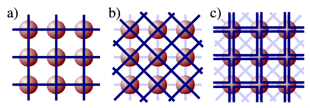
In defining SBS on higher dimensional systems, the choice of the subsets (called “strings” furtheron, as they impose a one-dimensional ordering in the spirit of MPS) is of central importance. The idea is that the string pattern should reflect the geometry of the system in such a way that spins which are closely coupled by the Hamiltonian are rather closely connected by a string. For a 2D square lattice, a natural choice is to first put strings on all rows (i.e., one row forms one string, corresponding to a product of MPS on rows) and then connect the rows by additionally placing one string per column. We call this pattern, as illustrated in Fig. 1a, lines. The lines pattern can be enhanced in two different ways by putting additional strings: First, one can put strings on all diagonals of the lattice (Fig. 1b), and second, one can choose strings which form small loops, encompassing all elementary plaquettes (i.e., blocks of spins, Fig. 1c; cf. [21] for a generalization of this ansatz); both of these extensions allow for a better control of the correlations with diagonal neighbors. The patterns generalize straightforwardly to lattices in 3D or with different geometries. Note that by continuously adding strings, we will eventually be able to describe all states as SBS, as can be seen by putting one long snail-like string on the lattice (i.e., describing the whole state as an MPS). Clearly, for good practical results, the strings should be chosen such that the relevant states are well approximated at an early stage of the pattern.
The computational resources of SBS scale favorable as compared to PEPS: For each string, a matrix trace (4) has to be computed which takes resources ( for OBC), with the length of the string. This has to be multiplied by the number of strings , giving a computational cost of . In particular, the scaling in the accuracy parameter compares favorably to the () scaling of the PEPS method for OBC (PBC).
Let us briefly note that although we motivated SBS as a higher-dimensional generalization of MPS, one can also regard them as a specialized case of PEPS. PEPS form the most natural generalization of MPS to two dimensions [4], they are known to approximate the states of interest well [23, 24], and have been applied successfully in numerical simulations [6, 7]. However, the scaling in the accuracy parameter is rather bad, preventing the application of PEPS to problems beyond 2D systems with OBC (note, however, that iPEPS have been applied successfully to investigate 2D systems in the thermodynamic limit [9, 10]). One way to resolve this problem is to look for subclasses of PEPS which allow for more efficient algorithms. Indeed, SBS form such a subclass of PEPS [20]: While general PEPS are described by tensor networks with general tensors , SBS with a lines pattern have tensors of the form . Note, however, that the structure of the tensors gets more and more rich as one places additional strings on the lattice, and thus, SBS can only be embedded in PEPS at a cost exponential in the number of strings; moreover, since SBS computations scale much more favorably in the accuracy parameter, even for a basic lines pattern SBS can outperform PEPS as they can reach much larger ’s.
III Variational method using string-bond states
In the previous section, we have introduced string-bond states (SBS) as a class of states which generalize MPS to two- and higher dimensional systems while allowing for an efficient computation of expectation values. In this section, we will show how SBS can be used to build a variational algorithm for simulating the ground states of quantum spin systems. Although the ability to efficiently compute expectation values is a necessary criterion, it is not sufficient: One also needs an efficient and practical way to evolve the SBS towards the ground state.
The basic idea of a variational algorithm based on SBS is to fix a family of SBS (i.e., fix a certain string pattern and the dimension of the underlying matrices) and try to find the state within this family which minimizes the energy of a given local Hamiltonian. Similar to DMRG or the variational method over PEPS, we will carry out the optimization in a local fashion: We start from some SBS, described by a number of three-index tensors as in (4), select one of the tensors – let us call it – and try to minimize the energy with respect to this tensor while keeping the others fixed. This procedure is repeated for all tensors over and over until the energy converges, i.e. a minimum within the family of states is reached.
To determine how to change the selected tensor such as to minimize the energy, we use the linearity of the string-bond states in the tensor to be optimized,
| (5) |
where we have explicitly denoted the dependence of the string-bond state on . denotes a quadratic form in , where is the vectorized form of , i.e. , and we use boldface to avoid confusion with vectors in state space. Minimizing (5) with respect to is a generalized eigenvalue problem and can be solved efficiently.
In order to sample and , define vectors and via the linear functionals
| (6) |
where is the initial value of the tensor . It follows that the matrices and in (5) can be expressed as
| (7) |
where , and thus determined by Monte Carlo sampling of and , respectively. Note that by virtue of this definition, we obtain the normalization .
However, there is a major problem with the approach of solving the generalized eigenvalue problem: Monte Carlo sampling and is relatively inaccurate as compared to e.g. the approximate contraction as done in the PEPS algorithm [4], and moreover, our estimates of and get less and less accurate for ’s far away from as we have sampled with respect to the distribution at . Specifically, already small errors in might lead to completely wrong minima for the generalized eigenvalue problem. While for the PEPS algorithm, this problem can be successfully overcome by truncating small eigenvalues of , this is impractical for a method based on Monte Carlo due to the comparatively large error.
To overcome this problem, we do not solve the generalized eigenvalue problem to compute the new , but rather compute the gradient of the energy with respect to and change slightly along this gradient such as to decrease the energy. First, this accounts for the fact that our sample of and , Eq. (7), is most accurate around , and as we will see, it moreover yields a formula where neither nor appear in the denominator, such that small absolute errors remain small. Another advantage will be that it is possible to gain a considerable speed-up when sampling all the gradients simultaneously and change all the tensors along their gradient simultaneously – this is possible since the gradients decouple to first order.
In order to determine the gradient of the energy with respect to around , consider a small variation (with ):
where we have used the normalization . Thus, the gradient turns out to be
| (8) |
[using ]. Substituting the sampling formulas (7) for and and using that [Eq. (6)], we finally obtain that
where we have defined
and the energy can be computed as
While the previous derivation holds for any ansatz where is linear in , there are some additional tricks which can be applied in the case of SBS to save computation time. To this end, note that all we have to know are , , and the ratio (this is sufficient to generate a random walk). For a particular tensor , the dependence of on (where denotes the state of the spin associated with ) can be expressed as
where is the product of all other matrices on the string containing as a function of the state of the spins, and contains the contributions from all other strings. Thus, we have that
and therefore (with the physical spin index)
This means that in order to compute for a given tensor , one only has to consider the string which contains , instead of having to look at all the strings.
Similarly, in order to compute , one can exploit that for local Hamiltonians, string-order operators, etc., where has only few elements, and e.g. for local Hamiltonians on a 2D lattice, each only differs at two adjacent sites from . Thus,
can again be computed as the ratio of the matrix product traces for only the two strings on which and differ, again reducing the computational effort. Computing also allows for optimizations, depending on the way the new configuration is constructed starting from . For the simplest scenario where only a single spin is flipped, again only the strings containing this very spin have to be considered, and similarly if e.g. a pair of spins is being flipped.
Finally, we gain a speed-up by computing the gradients for all tensors simultaneously; this is reasonable since the joint gradient of all tensors is nothing but the direct sum of the individual gradients, thus, changing all the tensor in direction opposite to the gradient by a small amount will decrease the energy to leading order. In this case, computation time is saved by the fact that the same sample drawn from can be used, and that has to be computed only once.
The full algorithms looks as follows: Fix a string pattern and corresponding bond dimensions, and choose initial configurations for all tensors. Then, iterate the following: 1) Compute the energy and its gradient with respect to all tensors. 2) Change all the tensors by some small amount in the direction given by the gradient. 3) Start over at 1) with the modified tensors. Iterate this until the change in energy becomes smaller than some threshold and declare convergence. In order to ensure that the step along the gradient is small enough, it is advisable to normalize the gradients such that the step remains small even for steep gradients.
Instead of declaring convergence of the algorithm when the energy does not change any more, one can try to increase the precision and see whether this leads to a further improvement in energy, and only declare convergence if it doesn’t. There are three possiblities to do so: First, one can increase the length of the Monte Carlo sample used for computing the energy and the gradient, second, one can try to decrease the stepwidth used to update the tensors along the gradient, and finally, one can try to extend the variational family of states either by increasing the bond dimension or by adding extra strings. In all cases, it is advisable to use the previously obtained optimum as the initial state.
IV Numerical results
In the following, we present numerical results obtained for two- and three-dimensional frustrated spin systems using string-bond states. In all cases, the Monte Carlo sampling was carried out using single spin flip, or adjacent spin swap, Metropolis updates. The autocorrelation time was at most 100 updates (for the structure factor of the - model in the frustrated regime), and considerably less for local observables or non-frustrated models, even in 3D. This allowed us to choose the Monte Carlo samples sufficiently long such that in all cases, the error bars were below what could be illustrated in the plots (local observables to at least 0.1%, and non-local observables to at least 1% accuracy). Note, however, that this only means that we have good control over the error we make in measuring observables on the given variational state; the major (and not so well controlled) error source in the method is thus the ability of the ansatz class to correctly describe the ground state, together with the question as to whether the variational method converges to the optimal state within the class.

IV.1 Simulation in 2D: The model
We have applied SBS to the simulation of the so-called - model,
where denotes nearest neighbors in a 2D square lattice, and nearest neighbors along the diagonal. This model arises e.g. in the context of the Hubbard model which is believed to underly high-temperature superconductivity [25], and has become one of the paradigmatic models to understand quantum phase transitions in frustrated spin systems [26].


For the simulation, we started from the patterns lines, then added diagonals, and finally loops. Fig. 2 shows how the energy improves as is increased and additional strings are added, for ; as on one can see, the improvement due to additional strings depends on the model under consideration. Note that for our simulations, we have used the invariance of the model, which implies that we can project our ansatz into the spin subspace (as there is a ground state with spin ). This can be understood as an SBS with one additional string which covers the whole lattice and enforces . In practice, we achieve the restriction by sampling from the subspace: we start from a configuration in this subspace and create new configurations by swapping a randomly chosen pair of spins; we have observed that this restriction led to a significant improvement in energy.
In Fig. 3, we show results for the ground-state energy of the - model on lattices of size , , and with open boundaries, which we compare with the values obtained using exact diagonalization () and the PEPS method [7] (, ). Fig. 4 shows the same numbers for the case of periodic boundaries, compared to the exact numbers [26] (, ). Let us note that for lattices, there are no numbers available to compare with. Typical ’s were for up to and to for , and .

The relative errors in energy corresponding to Figs. 3 and 4 are shown in Fig. 6. While the energies obtained using SBS are above the exact/PEPS data, the error does not seem to depend on the system size or the choice of boundaries, which suggests that the method should be equally applicable to larger and PBC systems.
Let us now see whether SBS can reproduce the correlation functions of the - model. To this end, we use the structure factor
| (9) |
is the Fourier transform of the two-point correlation functions , i.e., it reveals information about the relative alignment of the spins, this is, the order of the system [27]. The results for for PEPS with OBC, SBS with OBC, and SBS with PBC is diplayed in Fig. 5. Note that the OBC results exhibit the same characteristic properties for both PEPS and SBS, while the SBS results for PBC are significantly different in the region around , where the behavior of the model is not yet fully understood. It is believed that in this region, the system is in some kind of glassy phase. While a signature of this phase can be seen in the case of OBC both for the PEPS and the SBS data, the same signature is completely absent in the case of periodic boundaries. While this seems to suggest that the behavior of the system in that region might be different for OBC and PBC, we would like to stress that this is obtained from configurations with energies clearly above the exact and PEPS data, and thus should be treated with care.

IV.2 Three-dimensional systems
While some variational methods based on tensor networks such as PEPS [7], MERA [18], or Monte-Carlo based ansatzes such as SBS [20] or EPS [21] have been shown to be able to simulate two-dimensional frustrated quantum systems, none of the previous methods has yet be applied to the simulation of systems in three dimensions. In the following, we give results of SBS simulations for three-dimensional frustrated quantum systems which are comparable to those obtained in two dimensions.
The 3D simulations are based on the lines pattern on a 3D lattice with PBC, and . To benchmark the method, we have simulated the 3D Ising model with transverse field, , on an PBC lattice, and compared the result to QMC simulations carried out using the ALPS package [28, 29], as well as mean field data. Fig. 7 shows the magnetization along and the relative error in energy (inset) as a function of the field , and Fig. 8 the magnetization squared along the Ising coupling, . Note that the method becomes unstable close to the critical point and frequently gives too large values for . This is not a problem of the Monte Carlo sampling, which yields with an accuracy of about 1% (with Metropolis updates, where is sampled on every 100th configuration). Rather, this effect is due to the fact that variational methods using MPS and related ansatzed such as SBS generally tend to break symmetry close to the critical point even in 1D, as has been also observed elsewhere [30]. This can be understood in two ways: Firstly, the entanglement entropy of the ground state diverges at the critical point, so that the ground state cannot be exactly reproduced by states such as MPS or SBS which obey an area law, thus driving the ansatz into symmetry-broken solutions with slightly higher energy but less entanglement. Secondly, variational ansatzes have a general tendency to break symmetries as this corresponds to having less (connected) long-range correlations, and establishing such correlations is difficult to accomplish by doing local optimizations. E.g., in the most extreme case, once the matrices in the MPS or SBS do not have full rank any more, the subspace not used by the matrix is lost for the optimization as it cannot be seen any more by local variations, and in particular by a gradient search.


After having tested our 3D algorithm on the Ising model, we have subsequently applied SBS to simulate a frustrated XX model in a transverse field on a 3D square lattice,
| (10) |
where denotes nearest neighbors on the 3D square, and is chosen such that the system is frustrated around every plaquette, as illustrated in Fig. 9. There are several reasons for chooosing this model: First, it is frustrated and thus cannot be simulated by QMC due to the sign problem. Second, its lower symmetry as compared to an invariant model makes it easier to simulate. Finally, for this model, the magnetization is a good quantum number. Thus, the behavior of the model can be completely understood if the minimal energy for fixed at zero field is known: The minimal energy within each subspace with given magnetization decreases linearly with the field, , and the magnetization at a given is the one for which becomes minimal.
We have computed the for the model (10) on a lattice and from this data determined the ground state energy and the magnetization as a function of the field. The results are shown in Fig. 10, where we compare it to mean field data, which we also used to bootstrap the SBS ansatz. We found that most of the improvement is already obtained for ( being mean field), and for , the method was fully converged.
In order to estimate the performance of the ansatz, we have compared both mean field and SBS to the exact solution on a lattice. The results are shown in Fig. 11: While both energy and magnetization are still away from the exact solution, the values obtained using SBS are significantly more accurate than the mean field solution.
V Conclusions
In this work, we have presented numerical results obtained with the recently introduced String-Bond State (SBS) ansatz for frustrated quantum spin systems in both two and three dimensions and for open and periodic boundaries. While the results obtained for 2D OBC systems were above the results found using PEPS, the more favorable scaling of the method allowed us to go beyond 2D and OBC and obtain similarly accurate results for 2D PBC and 3D frustrated systems, which often cannot be simulated otherwise.
The computational resources needed for the simulation are moderate, as the contraction of the strings scales only with , and the ’s used are much smaller than those in DMRG; typical simulations for the - model took less than two days using a MATLAB code on a single processor. The method allows for parallelization in evaluating energy and gradient on the Monte Carlo sample with low interprocess communication. Optimizations are possible with respect to caching contracted strings and reusing them in consecutive Monte Carlo samples, as well as in reusing Monte Carlo samples after small updates.
There are two main challenges in the implementation of the algorithm. First, one needs a systematic way of growing the string pattern which is suitable for the problem at hand. As one can see in Fig. 2, the same string patterns lead to different improvements depending on the underlying model. Related to this, the performance of the method on non- invariant models will also depend on the choice of the local basis in which the sampling is performed, since this will affect the probability distribution sampled over. The second important point is to choose the proper initial state for the optimization. In particular, we have observed for the three-dimensional frustrated XX model presented in the paper that the algorithm performs much better when starting from the mean field solution as compared to a random initial state. Here, it seems that the important information is the proper sign of the wavefunction rather than the amplitude, as the latter can be easily changed by the gradient flow. (Note however that the performance for the - model did not depend on the choice of the initial state.) The proper choice of the sign pattern will likely also pose a central challenge when applying SBS to fermionic systems; note however that this might be overcome by using fermionic SBS, analogous to fermionic PEPS [31, 32], instead of mapping the system to spins via a Jordan-Wigner transform.
Acknowledgements
We thank F. Mezzacapo, F. Verstraete, and M. Wolf for helpful discussions and comments, S. Todo for help on the ALPS package, and V. Murg for providing us with the PEPS data. The Quantum Monte Carlo simulations of the 3D Ising model have been carried out using the ALPS looper code [28, 29], see http://alps.comp-phys.org and http://wistaria.comp-phys.org/alps-looper. This work has been supported by the EU (QUEVADIS, SCALA), the German cluster of excellence project MAP, the DFG-Forschergruppe 635, and the AXA Research Fund.
References
- [1] W. von der Linden, Physics Reports 220, 53 (1992).
- [2] S. R. White, Phys. Rev. Lett. 69, 2863 (1992).
- [3] U. Schollwöck, Rev. Mod. Phys. 77, 259 (2005), eprint cond-mat/0409292.
- [4] F. Verstraete and J. I. Cirac (2004), eprint cond-mat/0407066.
- [5] G. Sierra and M. A. Martin-Delgado, in Proceedings of the Workshop on the Exact Renormalization Group, Faro (Portugal) (1998), eprint cond-mat/9811170.
- [6] V. Murg, F. Verstraete, and J. I. Cirac, Phys. Rev. A 75, 033605 (2007), eprint cond-mat/0611522.
- [7] V. Murg, F. Verstraete, and J. I. Cirac, Phys. Rev. B 79, 195119 (2009), eprint arXiv:0901.2019.
- [8] A. Isacsson and O. F. Syljuasen, Phys. Rev. E 74, 026701 (2006).
- [9] J. Jordan, R. Orus, and G. Vidal, Phys. Rev. B 79, 174515 (2009), eprint arXiv.org:0901.0420.
- [10] B. Bauer, G. Vidal, and M. Troyer, J. Stat. Mech. p. P09006 (2009), eprint arXiv:0905.4880.
- [11] G. Vidal, Phys. Rev. Lett. 101, 110501 (2008), eprint quant-ph/0610099.
- [12] Z.-C. Gu, M. Levin, and X.-G. Wen, Phys. Rev. B 78, 205116 (2008a), eprint arXiv:0807.2010.
- [13] L. Wang, Y.-J. Kao, and A. W. Sandvik (2009), eprint arXiv:0901.0214.
- [14] H. C. Jiang, Z. Y. Weng, and T. Xiang, Phys. Rev. Lett. 101, 090603 (2008), eprint arXiv:0806.3719.
- [15] Z.-C. Gu, M. Levin, and X.-G. Wen, Phys. Rev. B 78, 205116 (2008b), eprint arXiv:0806.3509.
- [16] Z. Y. Xie, H. C. Jiang, Q. N. Chen, Z. Y. Weng, and T. Xiang, Phys. Rev. Lett. 103, 160601 (2009), eprint arXiv:0809.0182.
- [17] A. W. Sandvik, Phys. Rev. Lett. 101, 140603 (2008), eprint arXiv:0710.3362.
- [18] G. Evenbly and G. Vidal, Phys. Rev. Lett. 104, 187203 (2010), eprint arXiv.org:0904.3383.
- [19] A. W. Sandvik and G. Vidal, Phys. Rev. Lett. 99, 220602 (2007), eprint arXiv:0708.2232.
- [20] N. Schuch, M. M. Wolf, F. Verstraete, and J. I. Cirac, Phys. Rev. Lett. 100, 40501 (2008), eprint arXiv:0708.1567.
- [21] F. Mezzacapo, N. Schuch, M. Boninsegni, and J. I. Cirac, New J. Phys. 11, 083026 (2009), eprint arXiv:0905.3898.
- [22] H. J. Changlani, J. M. Kinder, C. J. Umrigar, and G. K.-L. Chan (2009), eprint arXiv.org:0907.4646.
- [23] M. B. Hastings, Phys. Rev. B 73, 085115 (2006), eprint cond-mat/0508554.
- [24] M. B. Hastings, Phys. Rev. B 76, 035114 (2007), eprint cond-mat/0701055.
- [25] M. Inui, S. Doniach, and M. Gabay, Phys. Rev. B 38, 6631 (1988).
- [26] H. J. Schulz, T. A. L. Ziman, and D. Poilblanc, J. Physique I 6, 75 (1996), eprint cond-mat/9402061.
- [27] A. Auerbach, Interacting electrons and quantum magnetism (Springer Verlag, New York, 1994).
- [28] S. Todo and K. Kato, Phys. Rev. Lett. 87, 047203 (2001).
- [29] A. Albuquerque, F. Alet, P. Corboz, P. Dayal, A. Feiguin, S. Fuchs, L. Gamper, E. Gull, S. Guertler, A. Honecker, et al., J. of Magn. and Magn. Materials 310, 1187 (2007), eprint arXiv:0801.1765.
- [30] C. Liu, L. Wang, A. W. Sandvik, Y.-C. Su, and Y.-J. Kao (2010), eprint arXiv:1002.1657.
- [31] C. V. Kraus, N. Schuch, F. Verstraete, and J. I. Cirac (2009), eprint arXiv:0904.4667.
- [32] P. Corboz, R. Orus, B. Bauer, and G. Vidal, Phys. Rev. B 81, 165104 (2010), eprint arXiv:0912.0646.