Learning networks from high dimensional binary data: An application to genomic instability data

Consider a $p\times 1$ vector of binary variables $X^{T}=(X_{1},\ldots,X_{p})$ for which we are interested in inferring the conditional dependencies. Here the superscript $T$ is a transpose. The pattern of conditional dependencies between these binary variables can be described by an undirected graph ${\cal G}=(V,E)$, where $V$ is a finite set of vertices, $(1,\ldots,p)$, that are associated with binary variables $(X_{1},\ldots,X_{p})$; and $E$ is a set of pairs of vertices such that each pair in $E$ are conditionally dependent given the rest of binary variables. We assume that the edge set $E$ doesn’t contain cycles, i.e., no path begins and ends with the same vertex. For example, in a set of four vertices, if the edge set includes (1,2), (2,3), and (3,4), it can’t include the edge (1,4) or (1,3) or (2,4), as it will form a cycle. Under this assumption, the joint probability distribution $\Pr(X)$ can be represented as a product of functions of pairs of binary variables. We formalize this result in the following proposition:

The proof of Proposition 1 is largely based on the Hammersley and Clifford theorem (Lauritzen, 1996) and given in Supplementary Appendix A.

Assuming $\Pr(X)$ is strictly positive for all values of $X$, then the above probability distribution leads to the well known quadratic exponential model

where $z^{T}=(x_{1}x_{2},x_{1}x_{3},\ldots,x_{p-1}x_{p})$, $\theta^{T}=(\theta_{1},\ldots,\theta_{p})$, $\kappa^{T}=(\kappa_{12},\kappa_{13},\ldots,\kappa_{(p-1)p})$, and $\Delta$ is a normalization constant such that $\Delta=\sum_{x_{1}=0}^{1}\cdots\sum_{x_{p}=0}^{1}\exp(x^{T}\theta+z^{T}\kappa)$.

Under this model, the zero values in $\kappa$ are equivalent to the conditional independence for the corresponding binary variables. The following proposition describes this result and the proof is given in Supplementary Appendix B.

As the goal of graphical model selection is to infer the edge set $E$ which represents the conditional dependence among all the variables, the result of Proposition 2 implies that we can infer the edge between a pair of events, say $X_{r}$ and $X_{s}$, based on whether or not $\kappa_{rs}$ is equal to 0. Interestingly, under model (1), $\kappa$ can also be interpreted as a conditional odds ratio. This can be seen from

Taking the log transformation of the left hand side of this equation results the familiar form of a logistic regression model, where the outcome is the $j$th binary variable and the predictors are all the other binary variables. Doing this for each of $x_{1},x_{2},\ldots,x_{p}$, we obtain $p$ logistic regressions models:

The matrix of all of the regression coefficients from $p$ logistic regression models can then be row combined as

with matrix elements defined by $\beta_{rs}$ for the $r$th row and the $s$th column of ${\cal B}$. It is easy to see that the $\cal{B}$ matrix is symmetric, i.e., $\beta_{rs}=\beta_{sr}=\kappa_{rs}$, $i\neq j$ under model (2.1). Vice versa, the symmetry of $\cal{B}$ ensures the compatibility of the $p$ logistic conditional distributions (2.1), and the resulting joint distribution is the quadratic exponential model (1)(Joe and Liu, 1986). Thus, to infer the edge set $E$ of the graphical model, i.e., non-zero off-diagonal entries in $\cal{B}$, we can resort to regression analysis by simultaneously fitting the $p$ logistic regression models in (2.1) with symmetric $\cal{B}$.

Specifically, let $X_{n\times p}$ denote the data which consists of $n$ samples each measured with $p$-variate binary events. We also define two other variables mainly for the ease of the presentation of the likelihood function: (1) $Y$ is the same as $X$ but with 0s replaced with -1s; (2) $X^{r},r=1,\ldots,p$ same as X but with $r$th column set to 1. We propose to maximize the joint log likelihood of the $p$ logistic regressions in (2.1) as follows:

where $X^{r}[i,]=(x^{r}_{i1},\ldots,x^{r}_{ip})$; and ${\cal{B}}[r,]=(\beta_{r1},...,\beta_{rp})$. Note, here we have the constraints $\beta_{rs}=\beta_{sr}$ for $1\leq r<s\leq p$; and $\beta_{rr}$ now represents the intercept $\theta_{r}$ of the $r$th regression.

Recall that our interest is to infer oncogenic pathways based on genome instability profiles of tumor samples. Most often, we are dealing with hundreds or thousands of genes and only tens or hundreds of samples. Thus, regularization on parameter estimation becomes indispensable as the number of variables is larger than the sample size, $p>n$. In the past decade, $\ell_{1}$ norm based sparsity constraints such as lasso (Tibshirani 1996) have shown considerable success in handling high-dimension-low-sample-size problems when the true model is sparse relative to the dimensionality of the data. Since it is widely believed that genetic regulatory relationships are intrinsically sparse (Jeong et al. 2001; Gardner et al. 2003), we propose to use $\ell_{1}$ norm penalty for inferring oncogenic pathways. The penalized loss function can be written as:

Note that $\ell_{1}$-norm penalty is imposed on all off-diagonal entries of $\cal{B}$ matrix simultaneously to control the overall sparsity of the joint logistical regression model, i.e., only a limited number of $\beta_{rs}$, $r\neq s$ will be non-zero. We then estimate $\cal{B}$ by $\widehat{\cal{B}}(\lambda):=\textrm{arg min}_{\cal{B}}l_{\lambda}^{lasso}({\cal{B}})$. In the rest of the paper, we refer to the model defined in (7) as LogitNet model, $\widehat{\cal{B}}(\lambda)$ as the LogitNet estimator and $\widehat{\beta}_{rs}(\lambda)$ as the $rs$th element of $\widehat{\cal{B}}(\lambda)$.

As described in the Introduction, the LogitNet model is closely related to the work by Ravikumar et al. (2009) which fits $p$ lasso logistic regressions separately (hereafter referred to as SepLogit). Our model, however, differs in two aspects: (1) LogitNet imposes the lasso constraint for the entire network while SepLogit does it for each neighborhood; (2) LogitNet enforces symmetry when estimating the regression coefficients while SepLogit doesn’t, so for LogitNet there are only about half of the parameters needed to be estimated as for SepLogit. As a result, the LogitNet estimates are more efficient and the results are more interpretable than SepLogit.

In this section, we describe an algorithm for obtaining the LogitNet estimator $\widehat{\cal{B}}(\lambda)$. The algorithm extends the gradient descent algorithm (Genkin et al. 2007) to enforce the symmetry of $\cal{B}$. Parameters are updated one at a time using a one-step Newton-Raphson algorithm, in the same spirit as the shooting algorithm (Fu, 1998) and the coordinate descent algorithm (Friedman et al., 2007a) for solving the general linear lasso regressions.

More specifically, let $\dot{l}(\beta_{rs})$ and $\ddot{l}(\beta_{rs})$ be the first- and second- partial derivatives of log-likelihood $l(\cal{B})$ with respect to $\beta_{rs}$,

where $R_{r}=X^{r}[i,]\beta^{T}[r,]Y[i,r]$. Under the Newton-Raphson algorithm, the update for the estimate $\widehat{\beta}_{rs}$ is $\Delta\beta_{rs}=-\dot{l}(\beta_{rs})/\ddot{l}(\beta_{rs})$. For the penalized likelihood (7), the update for $\widehat{\beta}_{rs}(\lambda)$ is

where $\mbox{sgn}(\beta_{rs})$ is a sign function, which is 1 if $\beta_{rs}$ is positive and -1 if $\beta_{rs}$ is negative. The estimates are also thresholded such that if an update overshoots and crosses the zero, the update will be set to 0. If the current estimate is 0, the algorithm will try both directions by setting sgn to be 1 and -1, respectively. By the convexity of (7), the update for both directions can not be simultaneously successful. If it fails on both directions, the estimate will be set to 0. The algorithm also takes other steps to make sure the estimates and the numerical procedure are stable, including limiting the update sizes and setting the upper bounds for $\ddot{l}$ (Zhang and Oles 2001). See Supplemental Appendix C for more details of the algorithm.

To further improve the convergence speed of the algorithm, we utilize the Active-Shooting idea proposed by Peng et al. (2009a) and Friedman et al. (2009). Specifically, at each iteration, we define the set of currently non-zero coefficients as the current active set and conduct the following two steps: (1) update the coefficients in the active set until convergence is achieved; (2) conduct a full loop update on all the coefficients one by one. We then repeat (1) and (2) until convergence is achieved on all of the coefficients. Since the target model in our problem is usually very sparse, this algorithm achieves a very fast convergence rate by focusing on the small subspace whose members are more likely to be in the model.

We note that in equation (5) the regularization shrinks the estimate towards zero by the amount determined by the penalty parameter $\lambda$ and that each parameter is not penalized by the same amount: $\lambda$ is weighted by the variance ${\ddot{l}(\beta_{rs})}^{-1}$ of $\widehat{\beta}_{rs}$. In other words, parameter estimates that have larger variances will be penalized more than the ones that have smaller variances. It turns out that this type of penalization is very useful, as it would also offer us ways to account for the other features of the data. In the next section we show a proposal for adding another weight function to account for spatial correlations in genomic instability data.

Spatial correlation of aberrations is common in genomic instability data. When we perform the regression of $X_{r}$ on all other binary variables, loci that are spatially closest to the $X_{r}$ are likely the strongest predictors in the model and will explain away most of the variation in $X_{r}$. The loci at the other locations of the same or other chromosomes, even if they are correlated with $X_{r}$, may be left out in the model. Obviously this result is not desirable because our objective is to identify the network among all of these loci (binary variables), in particular those that are not close spatially as we know them already.

One approach to accounting for this undesirable spatial effect is to downweight the effect of the neighboring loci of $X_{r}$ when regressing $X_{r}$ on the rest of the loci. Recall that in Section 2.2, we observed that the penalty term in (8) is inversely weighted by the variance of the parameter estimates. Following the same idea, we can achieve the downweighting of neighboring loci by letting the penalty term be proportional to the strength of their correlations with $X_{r}$. This way we can shrink the effects of the neighboring loci with strong spatial correlation more than those that have less or no spatial correlation. Specifically, the update for the parameter estimate $\beta_{rs}$ in (8) can be written as

where $w_{rs}$ is the weight for the spatial correlation. Naturally the weight $w_{rs}$ for $X_{r}$ and $X_{s}$ on different chromosomes is 1 and for $X_{r}$ and $X_{s}$ on the same chromosome should depend on the strength of the spatial correlation. As the spatial correlation varies across the genome, we propose the following adaptive estimator for $w_{rs}$:

1. 1.

   Calculate the odds ratio $\alpha$ between every locus in the chromosome with the target locus by univariate logistic regression.

2. 2.

   Plot the $\alpha$’s by their genomic locations and smooth the profile by loess with a window size of 10 loci.

3. 3.

   Set the smoothed curve $\widetilde{\alpha}$ to 0 as soon as the curve starting from the target locus hits 0. Here “hits 0” is defined as $\widetilde{\alpha}<\varepsilon$, where $\varepsilon=\textrm{median}_{r}|\widetilde{\alpha}_{r}-\widetilde{\alpha}_{r+1}|$.

4. 4.

   Set the weight $w=\exp(\alpha)$.

It is worth noting that the above weighting scheme together with the enforcement of the symmetry of $\cal{B}$ in LogitNet encourages a group selection effect, i.e., highly correlated predictors tend to be in or out of the model simultaneously. We illustrate this point with a simple example system of three variables $X_{1},X_{2}$, and $X_{3}$. Suppose that $X_{2}$ and $X_{3}$ are very close on the genome and highly correlated; and $X_{1}$ is associated with $X_{2}$ and $X_{3}$ but sits on a different chromosome. Under our proposal, the weight matrix $w$ is 1 for all entries except $w_{23}=w_{32}=a$, which is a large value because of the strong spatial correlation between $X_{2}$ and $X_{3}$. Then, for LogitNet, the joint logistic regression model

is subject to the constraint $|\beta_{12}|+|\beta_{13}|+a|\beta_{23}|<s$. Because of the large value of $a$, $\beta_{23}$ will likely be shrunk to zero, which ensures $\beta_{12}$ and $\beta_{13}$ to be nonzero in (10) and (11), respectively. With the symmetry constraint imposed on $\cal{B}$ matrix, we also enforce both $\beta_{12}$ and $\beta_{13}$ to be selected in (9). This grouping effect would not happen if we fit only the model (9) for which only one of $\beta_{12}$ and $\beta_{13}$ would likely be selected (Zou and Hastie 2005), nor would it happen if we didn’t have a large value of $a$ because $\beta_{23}$ would have been the dominant coefficient in models (10) and (11). Indeed, the group selection effect of LogitNet is clearly observed in the simulation studies conducted in Section 3.

We consider two procedures for selecting the penalty parameter $\lambda$: cross validation (CV) and Bayesian Information Criterion (BIC).

We generated background aberration events with spatial correlation using a homogenous Bernoulli Markov model. It is part of the instability-selection model (Newton et al. 1998), which hypothesizes that the genetic structure of a progenitor cell is subject to chromosomal instability that causes random aberrations. The Markov model has two parameters: $\delta$ and $\nu$, where $\delta$ is the marginal (stationary) probability at a marker locus and $\nu$ measures the strength of the dependence between the aberrations. So $\delta$ plays the role of a background or sporadic aberration when $\nu$ affects the overall rate of change in the stochastic process. Under this model, the infinitesimal rate of change from no aberration to aberration is $\nu\delta$, and from aberration to no aberration is $\nu(1-\delta)$. We then super-imposed the aberrations at disease loci, which were generated according to a pre-determined oncogenic pathway, on the background aberration events. The algorithm for generating an aberration indicator vector $X^{T}=(X_{1},\cdots,X_{p})$ is given below:

1. 1.

   Specify the topology of an oncogenic pathway for the disease loci and the transitional probabilities among the aberrations on the pathway. The $K$ disease loci are indexed by $\{{s_{1}},\cdots,{s_{K}}\}$, where $s_{i}\in\{1,\ldots,p\}$ for $i=1,\ldots,K$.

2. 2.

   Generate background aberrations denoted by a $p\times 1$ vector $Z$ according to the homogenous Bernoulli Markov process with preselected values of $\delta=0.05$ and $\nu=15$.

3. 3.

   Generate aberration events at disease loci following the oncogenic pathway specified in Step 1. This is denoted by a $p\times 1$ vector $U$, where indices $\{{s_{1}},\cdots,{s_{K}}\}$ are disease loci. If disease locus $s_{i}$ has an aberration ($U_{s_{i}}=1$), we also assign aberrations to its neighboring loci $U_{t}=1$, for $t\in[s_{i}-a_{i},s_{i}+b_{i}]$, where $a_{i}$ and $b_{i}$ are independently sampled from Uniform$[0,30]$. The rest of the elements in $U$ are 0.

4. 4.

   Combine the aberration events at disease loci and the background aberrations by assigning $X_{i}=1\textrm{ if }U_{i}+Z_{i}>0$ and $0\textrm{ if }U_{i}=Z_{i}=0$, for $i=1,\ldots,p$.

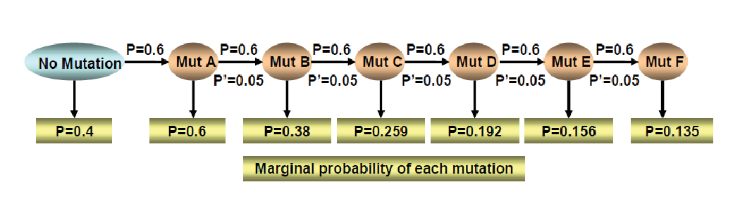
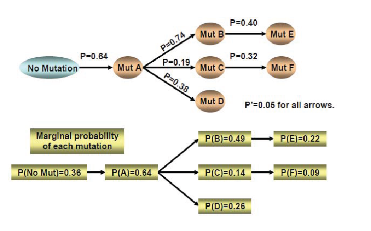
We set $n=200$ and $p=600$ to mimic the dimension of the real data set used in Section 4, so $V=\{1,\ldots,600\}$. We assume the $600$ marker loci fall into 6 different chromosomes with 100 loci on each chromosome. We consider two different oncogenic pathway models: a chain shape and a tree shape (see Figure 1). Each model contains 6 aberration events: $\texttt{M}=\{\texttt{A},\texttt{B},\texttt{C},\texttt{D},\texttt{E},\texttt{F}\}$. Without loss of generality, we assume these 6 aberrations are located in the middle of each chromosome, so the indices of A–F are $s_{\mathtt{A}}=50$, $s_{\mathtt{B}}=150$, $\cdots$, $s_{\mathtt{F}}=550$, respectively. For any $\texttt{u}\in\texttt{M}$, $X_{s_{\mathtt{u}}}=1$ means aberration u occurs in the sample.

We evaluate the performance of the methods by two metrics: the false positive rate (FPR) and the false negative rate (FNR) of edge detection. Denote the true edge set $E=\{(u,v)|X_{u}\mbox{ and }X_{v}\mbox{ are conditionally dependent },u\in V,v\in V\}$. We define a non-zero $\hat{\beta}_{rs}$ a false detection if its genome location indices $(r,s)$ is far from the indices of any true edge:

For example, in Figure 3 red dots that do not fall into any grey diamond are considered false detection. A cutoff value of 30 is used here because in the simulation setup (see Step 3) we set the maximum aberration size around the disease locus to be 30. Similarly, we define a conditionally dependent pair $(\texttt{u},\texttt{v})\in E$ is missed, if there is no non-zero $\beta$ falling in the grey diamond. We then calculate FPR as the number of false detections divided by the total number of non-zero $\hat{\beta}_{rs}$, $r<s$; and calculate FNR as the number of missed $(\texttt{u},\texttt{v})\in E$ divided by the size of $E$.

For the chain model, aberrations A-F occur sequentially on one oncogenic pathway. The aberration frequencies and transitional probabilities along the oncogenic pathway are illustrated in Figure 1(a). The true conditionally dependent pairs in this model are

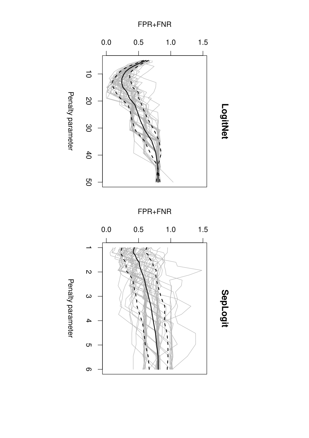
Based on this chain model, we generated 50 independent data sets. The heatmap of one example data matrix $200\times 600$ is shown in Supplemental Figure S-1. We then apply LogitNet and SepLogit to each simulated data set for a series of different values of $\lambda$. Figure 2 shows the FPR and FNR of the two methods as a function of $\lambda$. For both methods, FPR decreases with $\lambda$ while FNR increases with $\lambda$. Comparing the two methods, LogitNet clearly outperforms SepLogit in terms of FPR and FNR. For LogitNet, the average optimal total error rate (FPR$+$FNR) across the 50 independent data sets is 0.014 (s.d.=0.029); while the average optimal total error rate for SepLogit is 0.211 (s.d.=0.203). Specifically, taking the data set shown in the Supplemental Figure S-1 as an example, the optimal total error rate achieved by LogitNet on this data set is 0, while the optimal total error achieve by SepLogit is 0.563 (FPR$=0.563$, FNR$=0$). The corresponding two coefficient matrices $\hat{\cal{B}}$ are illustrated in Figure 3. As one can see, there is a large degree of asymmetry in the result of SepLogit: 435 out of the 476 non-zero $\hat{\beta}_{rs}$ have inconsistent transpose elements, $\hat{\beta}_{sr}=0$. On the contrary, by enforcing symmetry our proposed approach LogitNet has correctly identified all five true conditionally dependent pairs in the chain model. Moreover, the non-zero $\hat{\beta}_{rs}$’s plotted by red dots tend to be clustered within the grey diamonds. This shows that LogitNet indeed encourages group selection for highly correlated predictors, and thus is able to make good use of the spatial correlation in the data when inferring the edges.

We also evaluated the two penalty parameter selection approaches: CV and BIC, for LogitNet. Table 1 summarizes the FPR and FNR for CV and BIC. Both approaches performed reasonably well. The CV criterion tends to select larger models than the BIC, and thus has more false positives and fewer false negatives. The average total error rate (FPR$+$FNR) for CV is 0.079, which is slightly smaller than the total error rate for BIC, 0.084.

For the tree model, we used the empirical mutagenic tree derived in Beerenwinkel et al. (2004) for a HIV data set. The details of the model are illustrated in Figure 1(b). The true conditionally dependent pairs in this model are

The results of LogitNet and SepLogit for these data sets are summarized in Figure 4. Again, LogitNet outperforms SepLogit in terms of FPR and FNR. The average optimal total error rate (FPR+FNR) achieved by LogitNet across the 50 independent data sets is 0.163 (s.d.=0.106); while the average optimal total error rate for SepLogit is 0.331 (s.d.=0.160), twice as large as LogitNet. We also evaluated CV and BIC for LogitNet. The results are summarized in Table 1. Both CV and BIC give much higher FNRs under the tree model than under the chain model. This is not surprising as some transition probabilities between aberration events along the pathway are smaller in the tree model than in the chain model. As in the chain model, we also observe that BIC gives smaller FPR and higher FNR than CV, suggesting CV tends to select larger models and thus yields less false negatives but with more false positives in detecting edges.

References

- (1) Beerenwinkel, N., Rahnenführer, J., Däumer, M., Hoffmann, D., Kaiser, R., Selbig, J. and Lengauer, T. (2005). Learning Multiple Evolutionary Pathways from Cross-Sectional Data. Journal of Computational Biology 12, 584–598.
- (2) Cox, D.R. (1972). The analysis of multivariate binary data. Applied Statistics 21, 113–120.
- (3) Dawid, A.P. and Lauritzen, S.L. (1993). Hyper-Markov laws in the statisticla analysis of decomposable graphical models. Annals of Statistics 21, 1272–1317.
- (4) Drton, M. and Perlman, M.D. (2004). Model selection for Gaussian concentration graphs. Biometrika 91, 591–602.
- (5) Edward, D. (2000). Introduction to Graphical Modelling (2nd ed.), New York: Springer.
- (6) Efron, B., Hastie, T., Johnstone, I., and Tibshirani, R. (2004). Least Angle Regression. Annals of Statistics 32, 407–499.
- (7) Friedman, J., Hastie, T., Hofling, H., and Tibshirani, R. (2007a). Pathwise Coordinate Optimization. Annals of Applied Statistics, 1, 302–332.
- (8) Friedman, J., Hastie, T. and Tibshirani, R. (2007b). Sparse inverse covariance estimation with the graphical lasso. Biostatistics 9, 432–441.
- (9) Friedman, J., Hastie, T. and Tibshirani, R. (2009). Regularization Paths for Generalized Linear Models via Coordinate Descent. Technical report: http://www- stat.stanford.edu/ jhf/ftp/glmnet.pdf.
- (10) Fu, W. (1998). Penalized Regressions: the Bridge vs the Lasso. Journal of Computational and Graphical Statistics 7, 397–416.
- (11) Genkin, A., Lewis, D.D., Madigan, D. (2007). Large-scale Bayesian logistic regression for text categorization. Technometrics 49, 291–304.
- (12) Joe, H. and Liu, Y. (1996). A model for a multivariate binary response with covariates based on compatible conditionally specified logistic regression. Statistics & Probability Letters 31, 113–120.
- (13) Klein, G. and Klein, E. (1985). Evolution of tumors and the impace of molecular oncology. Nature 315, 190–195.
- Lauritzen (1996) Lauritzen, S.L. (1996). Graphical Models Clarendon Press, Oxford, United Kingdom.
- (15) Li, H. and Gui, J. (2006). Gradient Directed Regularization for Sparse Gaussian Concentration Graphs, with Applications to Inference of Genetic Networks. Biostatitics, 7, 302–317.
- (16) Loo, L., Ton, C., Wang, Y.W., Grove, D.I., Bouzek, H., Vartanian, N., Lin, M.G., Yuan, X., Lawton, T.L., Daling, J.R., Malone, K.E., Li, C.I., Hsu, L., Porter, P. (2008). Differential patterns of allelic loss in estrogen receptor-positive infiltrating lobular and ductal breast cancer. Genes, Chromosomes and Cancer 47, 1049–66.
- (17) Madigan, D. and York, J. (1995). Bayesian graphical models for discrete data. International Statistical Review 63, 215–232.
- (18) Meinshausen, N. and Buhlmann, P. (2006). High dimensional graphs and variable selection with the Lasso. Annals of Statistics 34, 1436–1462.
- (19) Newton, M.A., Gould, M.N., Reznikoff, C.A. and Haag, J.D. (1998). On the statistical analysis of allelic-loss data. Statistics in Medicine 17, 1425–1445.
- (20) Peng, J., Wang, P., Zhou, N. and Zhu, J. (2009a). Partial Correlation Estimation by Joint Sparse Regression Model. Journal of the American Statistical Association 104, 735–746.
- (21) Peng, J., Zhu, J., Bergamaschi, A., Han, W., Noh, D.Y., Pollack, J.R., Wang, P. (2009b). Regularized Multivariate Regression for Identifying Master Predictors with Application to Integrative Genomics Study of Breast Cancer. Technique Report http://arxiv.org/abs/0812.3671.
- (22) Prentice, R.L. and Zhao, L.P. (1991). Estimating equations for parameters in means and covariances of multivariate discrete and continuous responses. Biometrics 47, 825–839.
- (23) Ravikumar, P., Wainwright, M. and Lafferty, J. (2009). High-dimensional Ising model selection using -regularized logistic regression. Annals of Statistics to appear.
- (24) Rothman, A.J., Bickel, P.J., Levina, E. and Zhu, J. (2008). Sparse permu- tation invariant covariance estimation. Electronic Journal of Statistics 2, 494–515.
- (25) Schafer, J. and Strimmer, K. (2005). A Shrinkage Approach to Large-Scale Co- variance Matrix Estimation and Implications for Functional Genomics. Statistical Applications in Genetics and Molecular Biology, 4, Article 32.
- (26) Tibshirani, R. (1996). Regression shrinkage and selection via the lasso. Journal of the Royal Statististical Society Series B 58, 267–88.
- (27) Whittaker, J. (1990). Graphical Models in Applied Mathematical Multivariate Statistics. Wiley.
- (28) Wu, K., Katiyar, S., Witkiewicz, A., Li, A., McCue, P., Song, L., Tian, L., Jin, M., Pestell, R.G. (2009) The Cell Fate Determination Factor Dachshund Inhibits Androgen Receptor Signaling and Prostate Cancer Cellular Growth. Cancer Research 69, 3347–3355.
- (29) Yuan, M. and Lin, Y. (2007). Model Selection and Estimation in the Gaussian Graphical Model. Biometrika 94, 19–35.
- (30) Zhang, T. and Oles, F. (2001). Text categorization based on regularized linear classifiers. Information Retrieval 4, 5–31.
- (31) Zhao, L.P. and Prentice, R.L. (1990). Correlated binary regression using a quadratic exponential model. Biometrika 77, 642–648.
- (32) Zou, H., Hastie, T. (2005). Regularization and variable selection via the elastic net. Journal of the Royal Statistical Society, Series B 67, 301–320.
- (33) Zou, H., Hastie, T., Tibshirani, R. (2007). On the degrees of freedom of the lasso. Annals of Statistics 35 2173–2192.