Hadrons and direct photon in pp and pA collisions at LHC and saturation effects
Abstract
We investigate hadrons and direct photon production in and collisions at the energies of RHIC and LHC within the color-dipole approach employing various saturation models. We show that greatest sensitivity to saturation effects is reached at very forward rapidities for collisions at LHC ( TeV). The ratio of direct-photon to pion production can be about (at ). Therefore, direct photon production at forward rapidities should provide a rather clean probe. We calculate the rapidity dependence of the invariant cross-section and find some peculiar enhancement at forward rapidities which is more pronounced for direct photon production. We show that this peak is further enhanced by saturation effects. We provide predictions for the nuclear modification factor for pions and direct photon production in collisions at LHC energy at midrapidity. We show within various saturation models that the pion Cronin enhancement at RHIC is replaced by a moderate suppression at LHC energy at midrapidity due to gluon shadowing effects. Cronin enhancement of direct photons can survive at LHC energy within models with a larger saturation scale.
August 24, 2026
I Introduction
The Large Hadron Collider (LHC) will allow to explore a new regime of QCD where parton saturation effects become important [1, 2, 4, 3, 5]. At the same time, the physics of saturation might also be relevant for a detailed understanding of the underlying events, i.e. the backgrounds for New Physics searches at LHC.
It is believed that and collisions provide a testing ground to disentangle the initial- and final-state effects in collisions and can be used as a baseline for understanding the physics of heavy-ions collisions. For example, to interpret jet-quenching, a precise and firm understanding of the Cronin, shadowing and saturation effects in collisions is indispensable.
The Color Glass Condensate (saturation) approach to QCD at high energy [1, 2, 4, 3, 5] has been very successful to describe a variety of processes at Relativistic Heavy Ion Collider (RHIC) [6](for a review see [5] and references therein). Nevertheless, the importance of saturation effects is still disputable given that other approaches offered alternative descriptions, see for example Refs. [7, 8]. In order to test saturation physics and its relevance, it seems therefore mandatory to consider various reactions in different kinematic regions at LHC and future collider experiments.
Here, we study hadron and direct photon production in and collisions within the light-cone color-dipole formulation and investigate the role of saturation and shadowing at LHC energies. The corresponding phenomenology is based on the universal dipole cross-section. The dipole cross-section incorporates the multiple gluon scattering and non-linear gluon recombination effects and can be in principle measured in deep-inelastic scattering (DIS), see section VI. In the parton model language, the dipole cross-section plays the role of leading twist parton distributions in an all twist environment.
Direct photons (photons radiated in hadronic collisions not via hadronic decays) carry important information about the collision dynamics which is undisturbed by final state interactions. We compare hadron and direct photon production mechanisms at various energies and rapidities in collisions. We show that the ratio of photon/pion production at very forward rapidities grows and can become as big as one order of magnitude at the LHC energy TeV. Measurements of direct photons at forward rapidities should be rather clean, as the background from radiative hadronic decays is significantly suppressed11 1 Experimentally measurements at forward rapidities are a challenge since production rates are lower due to kinematic limits.. At the same time, we show that both hadrons and direct photons are sensitive to saturation effects at forward rapidities at TeV collisions.
We also investigate the role of saturation and shadowing effects for hadron and direct photon production in collisions at LHC. Our approach gives a rather fair description of PHENIX data for the Cronin ratio of pions. We show that the nuclear modification factor for at LHC ( TeV) at midrapidity becomes less than in all saturation color-dipole models due to gluon shadowing. The suppression obtained (for ) in our approach is less than the one predicted in the Color Glass Condensate (CGC) approach [9]. We will later highlight the difference between our results and other reported predictions. We will also show that the nuclear modification factor for direct photons is also less than within the CGC color-dipole model once shadowing effects are included. In contrast, the Cronin enhancement for photons can survive even after inclusion of shadowing effects within the Golec-Biernat and Wüsthoff color-dipole model which has a bigger saturation scale than the CGC model.
The paper is organized as follows: In Sec. II and III we calculate gluon radiation from projectile gluons and quarks in the color-dipole approach. In Sec. IV we introduce the light-cone color-dipole factorization scheme for hadron production. In Sec III, IV we will also highlight the differences between our approach with others. In Sec V we calculate the direct-photon production in and collisions. In Sec VI we introduce gluon saturation within various approaches and color-dipole models. In Sec VIII we discuss nuclear gluon shadowing, Cronin effect and nuclear modification factor for partons, pions and direct photon production. In Sec VII and VIII we present our numerical results for both hadron and direct-photon production in and collisions, respectively. As a conclusion, in Sec. IX we highlight our main results and predictions for LHC.
II gluon radiation by a projectile gluon:
The underlying mechanisms of the multiple particle interactions is controlled by the coherence length . In the incoherent case, the multiple interaction amplitude can be simplified as convolution of differential cross sections while in the coherent case, one should convolute scattering amplitudes rather than differential cross-sections.
The coherence length can be estimated from the inverse longitudinal momentum transfer,
| (1) |
where is the initial parton energy and is the relative transverse momentum of the final partons. In the above equation, is the invariant mass of the two final partons, neglecting parton masses. The parameter is the fractional light-cone momentum of one of the final partons. Gluon radiation is dominated by small values of , therefore we have,
| (2) |
where is the energy of the parton detected in the final state, is the transverse momentum of the fragmented hadron at midrapidity, and is the nucleon mass. For pion production, the average momentum fraction in the fragmentation functions is about in the range of . For a coherence length which is shorter than the typical internucleon separation (where denotes the nuclear radius), the projectile interacts incoherently. At the RHIC energy and intermediate we are almost in the transition region between the short- and long-coherence length regime. In more central collisions, at higher we are in the short-coherence length (SCL) limit and at LHC energies at moderate we are again in the long-coherence length (LCL) limit.
There is much experimental evidence for a large intrinsic momentum of gluons, see Refs. [10, 11] and reference therein. Therefore, interaction with spectators is important since color screening is at work. At smaller and moderate one should then include interaction with spectators, i.e. instead of ”elastic” gluon scattering, , we need to consider bremsstrahlung subprocesses, , or . The lowest order for these processes includes the three graphs shown in Fig. 1 (interactions with the initial and two final partons). After summing over radiated gluons, the cross section of this reaction can be expressed in terms of the color-dipole amplitudes [10, 12], and can be diagonalized for a nuclear target provided that the coherence length is sufficiently long. Note that since parton trajectories before and after gluon (or photon) radiation have different impact parameters, and the corresponding terms in the bremsstrahlung amplitude have different signs, one arrives at an expression, which is formally identical to the amplitude of an inelastic dipole-target interaction. This is only a formal procedure of calculation, while no real color-dipole is involved in the process of radiation contrary to DIS where a photon does split into a real pair.

In the LCL regime, the transverse momentum spectra of gluon bremsstrahlung for a high energy gluon interacting with a nucleon N (or nucleus A) including the nonperturbative interactions of the radiated gluon reads [10, 12],
| (3) | |||||
where denotes the light-cone momentum fractional of the radiated gluon. The partial amplitude of a -gluons system colliding with a proton at impact parameter can be written in terms of the dipole amplitude [13, 14],
| (4) | |||||
where the factor is the ratio of Casimir factors. Here the vectors , and denote the two gluon transverse separations , and , respectively.
Note that Eq. (4) can be simply understood by looking at several limiting cases: if goes to zero, the transverse separation of final state gluons and becomes zero leading to which reflects the fact that a point like gluon-gluon fluctuation cannot be resolved by interactions. In the two limiting cases of , the three-gluon system will be reduced to the two-gluon system which can be then related to the dipole cross-section via the Casimir factor: where is the ratio of the octet and triplet color Casimir factor.
The dipole amplitude in Eq. (4) is related to the dipole-proton cross-section by integration over impact parameter,
| (5) |
We still have to specify the light-cone distribution function () for the Fock component fluctuations of the incoming gluon, which includes nonperturbative interactions of these gluons. The light-cone wave function of the gluon-gluon (and quark-gluon) Fock component of a gluon (quark) was calculated in Ref. [10] within a model describing the nonperturbative interaction of gluons via a phenomenological light-cone potential of an oscillatory form. This is given by,
where is the parameter characterizing the strength of the nonperturbative interaction which has been fitted to data on diffractive scattering [10]. In Eq. (3) the product of the wave functions is averaged over the initial gluon polarization, , and summed over the final ones, .
Based on pQCD one might expect that the gluon-gluon potential differs from the quark-antiquark one simply by a Casimir factor . However, there exists plenty of evidence indicating that the interaction of gluons is much stronger due to non-trivial properties of the QCD vacuum, see Ref. [11] and references therein. It turns out that the exact shape of the light-cone gluon-gluon (quark-gluon) potential is not crucial [10]. What is only important is the smallness of the mean quark-gluon separation which defines the effective strength of gluons interaction. The value of fm obtained from analysis of diffractive data [10] agrees with both lattice calculations [15] and also with the phenomenological model of the instanton liquid [16].
We consider here the asymptotic expression of the gluon radiation cross-section given in Eq. (3) for which is reliable at very long coherence lengths. This is certainly valid at LHC energies. At RHIC energies, for hadrons produced at midrapidity with moderate , we are in the transition region between the regimes of long and short coherence lengths. Moreover, the color-dipole models we use in this paper, were fitted to DIS data at very small Bjorken-x , which corresponds to GeV at RHIC. Therefore, the prescription presented here should be less reliable at high- at RHIC energy. We will come back to this point in Sec. VIII.
After some algebra one obtains,
| (7) | |||||
where the function is defined as
| (8) | |||||
In the case of a nuclear target the functional form of Eq. (3) still holds, but the dipole amplitude for a nucleon target should be replaced by the one for a nuclear target . The partial elastic amplitude for a colorless three-gluon system colliding with a nucleus can be written in terms of the partial amplitude of a three-gluon system colliding with a proton at impact parameter ,
where the -gluons amplitude is related to the dipole amplitude via Eq. (4) and is the nuclear thickness function normalized to . In a very similar fashion as for the nucleon target case, one can analytically carry out some of the integrals,
| (10) | |||||
with the notation,
| (11) | |||||
where in the second line we used Eq. (5) and ignored possible correlations between the color-dipole amplitude and nuclear thickness. Notice that the second line were identically true if the nuclear profile would be a constant. In a more sophisticated approach in order to properly incorporate the correlation between the color-dipole amplitude and the nuclear thickness, one should also have a model for the dipole amplitude which depends on the angle between the dipole transverse radius and the impact parameter . Unfortunately, with available HERA data, it is difficult to incorporate the color-dipole orientation and most dipole models fitted to HERA data depend only on the absolute value of the transverse dipole size and impact parameter . For a recent attempt to incorporate the color dipole orientation, see Ref. [17]. It has been shown that the color-dipole orientation gives rise to azimuthal asymmetries [17], but is unimportant for total cross-sections.
III gluons radiation by a projectile quark:
Gluon radiation of a projectile quark interacting with a nucleon(nucleus) can be calculated in a similar way as outlined in the previous section. The cross-section is given by [10, 12],
where and are the quark-gluon transverse separation in the direct and complex conjugated amplitude respectively. For brevity, we define again as the fractional LC momentum of the radiated gluon, .
In Eqs. (3,) we have already integrated over the transverse coordinates of the second parton. Note that the formulas in Eqs. (3,) are given in impact parameter representation and contain the sum of diagrams given in Fig. 1. The derivation of these equations can be found in Refs. [10, 12]. The collinear divergences which are the source of scale dependence of the parton distribution functions and fragmentation functions in the factorization Eq. () are already subtracted in these equations.
The interaction amplitude of a colorless and system with a nucleon target can be written in terms of dipole amplitudes [13],
| (13) | |||||
| (14) |
Again likewise Eq. (4), the above equations immediately satisfy several simple limiting cases. When the transverse separation goes to zero i.e. , the pair is indistinguishable from a gluon, and Eq. (13) correctly reduces to . Moreover, in the limit of vanishing (or ), the (or ) system is indistinguishable from a quark (antiquark) and Eq. (13) becomes .
In the derivation of Eqs. (3, ), one can rearrange the final result in terms of Eqs. (4,13,14). However, this is more than just some change of notation since the combination of the right-hand sides of Eqs. (4,13,14) are already well-known as forward scattering amplitudes of , and system interacting with a proton target. Eqs. (4,13,14) are exact and are not based on any approximation. A formal derivation of these equations is similar to the derivation of the -proton dipole cross-section, namely one replaces the system by a (or , ) one. The exchanged gluons can now couple to different partons in the system (or , ) which generates different phase factors. The precise calculation of the color traces for the different couplings of the exchanged gluons to the quark, antiquark and gluon ( or 3-gluons, gluon-gluon) leads to the exact expression given in Eqs. (4,13,14) [10, 12, 13, 14]. Notice that in the CGC approach the relations Eqs. (4,13,14) holds only if one assumes that the weight function for averaging over the target color charges are Gaussian [18].
The forward scattering amplitude of , and interacting with a nucleus target at impact parameter , can be again written, in eikonal form, in terms of the dipole elastic amplitude of a dipole colliding with a proton at impact parameter ,
| (15) | |||||
| (16) | |||||
| (17) |
The light-cone distribution of quark-gluon fluctuations in Eq. () is given in Ref. [10]. In the limit which is of practical interest at high energy, the quark-gluon distribution function including non-perturbative effects has the form,
| (18) |
where the parameter fm denotes the mean quark-gluon separation and is the result of a fit to soft diffraction .
One can show that for the cross-section of gluon bremsstrahlung from projectile quarks is times smaller than the corresponding cross-section for a projectile gluon given by Eqs. (3,II,,18) due to the color factor:
| (19) |
Note that similar results as Eqs. (3,) was also obtained by Jalian-Marian and Kovchegov [19] in a color glass condensate picture where the color dipole amplitudes in Eqs. (3,) are replaced by a product of two Wilson lines evaluated in the field of the color glass condensate. See also Ref. [20] for an earlier attempt along this line. Loosely speaking, these two formulations are equivalent in the quasi-classical (Glauber) approximation. However, in order to include small-x evolution, it is not sufficient to only put Wilson lines in the evolved CGC fields. This only leads to logs of energy in the rapidity interval between the produced gluon and the nucleus. One should also include the evolution in the rapidity interval between the projectile and the produced gluon [21], thus describing gluon emission. It was shown by Kovchegov and Tuchin [21] that such an evolution is the linear BFKL equation due to some very interesting cancellations of all nonlinearities.
In our approach, the effects of gluon emissions between the quark (gluon) and the produced gluon (and its evolution) are effectively included in the master Eqs. (3,) via the non-perturbative quark-gluon (gluon-gluon) light-cone distribution functions Eqs. (II,18) which is obtained from a fit to soft diffraction data. The diffractive excitation of the incident hadrons to the states of large mass is a more sensitive probe of gluon-gluon fluctuations than the total cross section [10]. While the gluon emissions between the projectile and target including their non-linear recombination effects are effectively incorporated in terms of color-dipole forward amplitudes obtained from a fit to DIS data. By means of Eqs. (3,) one can also describe the long-standing problem of the small size of the triple-pomeron coupling [10, 11].
A word of caution is in order here. Notice that although the non-perturbative and light-cone distribution functions include some saturation effects of the projectile proton [10, 11]. Nevertheless, the gluon production cross-section given by Eqs. (3,) is intrinsically asymmetric, namely it treats the ”projectile” proton approximately in a collinear factorization framework while treating the ”target” proton (or nucleus) in a saturation framework. Strictly speaking this may be justified only in the case when saturation effects are present in the target wave function, but are absent in the projectile wave function, such as in collisions or in forward particle productions. Although it appears that such a simple approximation is sufficient to describe the existing experimental data for hadron and direct photon production at small at midrapidity in collisions, see Figs. 3, 6. Nevertheless, our formulation at midrapidity in collisions is not well justified and therefore our results at midrapidity in collisions may not be valid.
IV Hadrons production in high-energy and collisions
The cross section of hadron production in (or ) collisions at impact parameter is given by a convolution of the distribution function of the projectile gluon or quark inside the proton with the gluon radiation cross-section coming from or ( or ) collisions and also with the fragmentation functions. For simplicity, we assume here that the projectile gluon/quark has the same impact parameter relative to the target as the beam proton. This is certainly a rather poor approximation which we will try to improve upon in future.
and are the parton distribution functions (PDF) of the colliding protons, which depend on the hard scale and the light-cone momentum fractions and for quarks and gluons, respectively. The function is the fragmentation function of parton to the final hadron with a momentum fraction . In the above equation, the variables and are momentum fractions of a parton in the beam and target. The variables are defined by,
| (21) |
where and are the transverse momentum and rapidity of the produced hadron.
In Eq. () the cross-sections of gluon radiation in and are given by Eqs. (3,). We assume that the projectile parton acquires high transverse momentum as a result of coherent multiple rescattering, while the radiated gluons that generate this momentum are summed to build up the color dipole cross-section. Then, explicit inclusion of gluon bremsstrahlung balances the large .
Notice that in the dipole approach in contrast to the parton model, one should rely on the parton distribution functions taken at a soft scale since the evolution to the hard scale is performed via gluon radiation, which is encoded in the phenomenological dipole cross-section fitted to DIS data for the proton structure function. However, the dipole cross-section misses the -evolution of the -distribution, which is especially important at forward rapidities, since the parton distributions fall off at much steeper at high . In order to account for this effect and provide the correct -distribution, we take the integrated parton distribution in Eq. () at the hard scale [22, 23].
Notice that at high energies and midrapidity the parton fractional momenta in the beam and target are small, , so hadron production is dominated by fragmentation of radiated gluons . However, at very forward rapidities the quark contributions are important and the subprocess becomes relevant. Therefore, different subprocesses dominate in different kinematic regimes and their overlap is small.
V Photon radiation in high-energy and collisions
Production of direct photons in the target rest frame should be treated as electromagnetic bremsstrahlung by a quark interacting with the target. In the light-cone dipole approach the transverse momentum distribution of photon bremsstrahlung by a quark propagating and interacting with a target nucleon (or nucleus ) at impact parameter , as calculated from the diagrams in Fig. 1 (we show only the single gluon exchange diagrams), can be written in the factorized form [12, 22, 23]
| (22) | |||||
where and are the quark-photon transverse separations in the direct and complex conjugated amplitudes respectively; denotes the fractional light-cone (LC) momentum of the radiated photon. Correspondingly, the transverse displacements of the recoil quarks in the two amplitudes are and respectively. In Eq. (22), is the light-cone (LC) distribution amplitude of the projectile quark fluctuation. Averaging over the initial quark polarizations and summing over all final polarization states of the quark and photon, we get
| (23) | |||||
where denotes modified Bessel functions of the second kind and is an effective quark mass, which can be regarded as a cutoff regularization. Following Refs. [22, 23, 24] we take GeV. The forward scattering amplitude can be again written, in the eikonal form, in terms of the dipole elastic amplitude of a dipole colliding with a proton at impact parameter as defined in Eq. (15).
In order to obtain the hadron cross-section from the elementary partonic cross section Eq. (22), one should sum the contributions from quarks and antiquarks (since only quarks and antiquarks can radiate photons) weighted with the corresponding parton distribution functions. The PDFs of the projectile enter in a combination which can be written in terms of proton structure function . Notice that the contribution of gluon splitting to quark-antiquark pairs (and higher Fock components) is already contained in the sea quark distributions of the proton. Therefore, the direct-photon production cross-section in and collisions is given by [24, 22, 23],
where the variable and are defined in Eq. (21) and is the Feynman variable. We have recently shown that in this framework one can obtain a good description of the cross-section for prompt photon production in proton-proton collisions at RHIC and Tevatron energies [22, 23], and Drell-Yan dilepton pair production [22, 25]. Here, we employ this formulation to give predictions for the ratio of photon/pion production cross-sections at various rapidities for LHC. We will also provide prediction for the nuclear modification factor in collisions at LHC.
Notice that in the color-dipole factorization Eqs. (,V) neither K-factors (next-to-leading-order corrections), nor higher twist corrections should be added. The phenomenological dipole cross-section fitted to DIS data should already incorporate all perturbative and non-perturbative radiation processes. The only contribution which is still missing in Eq. (V) is the effect of the primordial momentum of the projectile parton. However, it has been shown that in the color-dipole approach, the primordial momentum should have a purely non-perturbative origin, and is considerably smaller than in the parton model [22, 23]. This effect should be of little importance for the kinematic regions of interest of this paper.
A word of caution is in order here. The type of factorization scheme outlined above Eqs. (,V) has not been yet rigorously proven at any order of pQCD in the kinematic region of our interest and is most probable not exact. Nevertheless, there is growing evidence in the literature that it gives a good approximation for the processes discussed here [7, 10, 12, 26, 27, 28, 22, 23, 24, 25].
VI Gluon saturation and color dipole models
At high energies/small Bjorken-x, QCD predicts that gluons in a hadron wavefunction form a new state, the so-called Color Glass Condensate (CGC) [1, 2, 4, 3, 5]. The cornerstone of the CGC is the existence of a hard saturation scale at which nonlinear gluon recombination effects become important and start to balance gluon radiation.
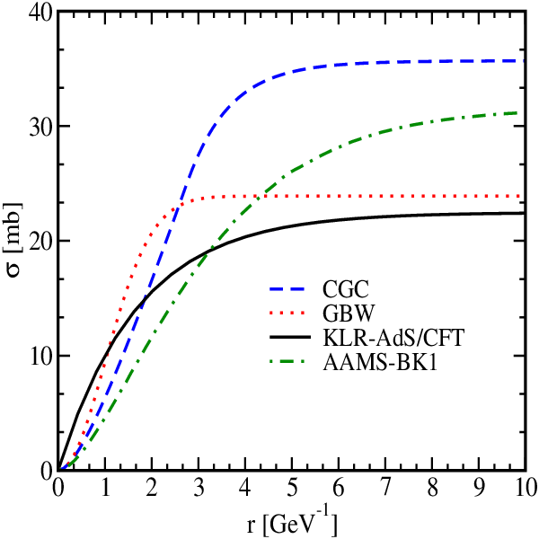
The concept of saturation and the taming of the power-like rise of the gluon distribution at small was first addressed by Gribov, Levin and Ryskin in the double logarithmic approximation [1]. A first hint toward saturation effects at HERA came from the phenomenologically success of the Golec-Biernat and Wüsthoff (GBW) model [29]. This model incorporates the basic saturation effects into the color-dipole cross-section on a proton target. In the CGC framework the dipole-proton forward scattering amplitude can be in principle found by solving the perturbative nonlinear small-x Balitsky-Kovchegov (BK) [3] or Jalilian-Marian–Iancu–McLerran–Weigert–Leonidov–Kovner (JIMWLK) [4] quantum evolution equations. The BK and JIMWLK evolution equations unitarize the linear Balitsky-Fadin-Kuraev-Lipatov (BFKL) [30] evolution equation at small- in the large- limit (BK) and beyond (JIMWLK). It has been shown that next-to-leading-order (NLO) corrections to the BFKL equation (and therefore to BK and JIMWLK kernels) are large and negative [31]. There was no reason to believe that still higher order corrections are unimportant, until quite recently, when it was found that the consistent incorporation of the running coupling into the BFKL, BK and JIMWLK equations [32, 33, 34] leads to phenomenologically rather successful descriptions. Still the actual calculation of higher-order corrections to these non-linear evolution equations remains as a challenge. Thus, we resort to a QCD-like model which incorporates the basic features of gluon saturation into the dipole-proton forward scattering amplitude, and provides predictions which will allow to test the validity of our treatment. There are several parametrizations proposed in the literature which all give a good description of HERA data but predict different saturation scales, see Fig. 2. In this section we review some of these models and later we will employ them for hadron and photon production in various kinematic regimes and investigate the uncertainties of the various models and discuss the differences between them.
VI.1 GBW model
The dipole-proton cross-section is usually written as an integral of the imaginary part of the forward scattering amplitude over the impact parameter as defined via Eq. (5). One may neglect the -dependence in making the integral in Eq. (5) trivial, giving the proton’s transverse area factor:
| (25) |
A popular parametrization for the dipole cross-section on a nucleon target is due to Golec-Biernat and Wüsthoff (GBW) [29] and is able to describe DIS data with a simple form for the color dipole amplitude,
| (26) |
where the -dependence of the saturation scale is given by
| (27) |
The main feature of the model is that for decreasing , the dipole amplitude saturates at smaller dipole sizes. Note that there is no unique definition for the saturation scale in literature. Following Refs. [29, 35, 36, 37] we define the saturation scale as a energy scale at which the dipole scattering amplitude becomes sizable,
| (28) |
For the GBW model, this definition coincides with the saturation scale defined in Eq. (27). The value of the intercept is consistent with perturbative predictions based on small-x evolution [39, 32, 34, 38, 40]. The parameters mb, , and were determined from a fit to for and in the presence of charm quarks with mass GeV [36]. Note that the saturation scale in the GBW model reduces with the inclusion of the charm quark [36].

VI.2 CGC, AAMS-BK and b-CGC models
The linear DGLAP evolution equation which only includes gluon radiation may not be appropriate for the saturation regime where nonlinear recombination subprocess are important. Iancu, Itakura and Munier proposed an alternative color glass condensate (CGC) model [41], based on the BK equation [3]. In this model the dipole amplitude for a nucleon target is parametrized as,
| (29) |
where the saturation scale is again parametrized as Eq. (27), , and where is the LO BFKL characteristic function. The coefficients and in the second line of (29) are determined uniquely from the condition that the color dipole cross-section and its derivative with respect to are continuous at :
| (30) |
The parameters and are fixed at the LO BFKL values. The others parameters , mb, and were fitted to for and and including a charm quark with GeV. Notice that for small , the effective anomalous dimension in the exponent in the upper line of Eq. (29) rises from the LO BFKL value towards the DGLAP value.
Recently, Albacete, Armesto, Milhano and Salgado calculated numerically the dipole-proton scattering amplitude from the BK equation including running coupling corrections (AAMS-BK1,2 model) [34]. Note that the incorporating of the running coupling is essential in this approach, though its implementation is model dependent. The free parameters in their fit to HERA data are related to the initial condition for the evolution at . They used two families of initial conditions, the GBW form (AAMS-BK1 model)
| (31) |
and the McLerran-Venugopalan form (AAMS-BK2 model):
| (32) |
where is the initial saturation scale. In their global analysis of HERA data there are four free parameters which are fitted to -data for and : the initial saturation scale , the overall normalization , the infrared parameter introduced in the running coupling and the anomalous dimension . The values of parameters can be found in table of Ref. [34].
The gluon density is larger in the center of a proton than at periphery probed in the total cross-section. Therefore, impact-parameter dependence of the dipole-proton forward scattering amplitude seems to be essential. There has been several attempts to model the impact-parameter dependence in dipole-proton forward scattering amplitudes. We consider here the model proposed by Watt and Kowalski (b-CGC) [42]. In this model, the dipole-proton forward scattering amplitude has the same form as the CGC model Eq. (29), but the saturation scale now depends on impact parameter,
| (33) |
The parameter is fitted to the -dependence of exclusive photoproduction. It has been shown that if one allows the parameter to vary together with the other parameters (in contrast to the CGC fitting procedure where is fixed to its LO BFKL value), this results in a significantly better description of data for with the value of , which is remarkably close to the value of recently obtained from the BK equation [43]. Other parameters obtained from the fit are: , and [42].
Notice that calculation of the -distribution of produced hadrons/photons in collisions needs only knowledge of the total dipole cross-section and is independent of the impact-parameter dependence of the forward scattering dipole-proton amplitude. Nevertheless, the integrated dipole cross-section of the b-CGC model is different from other dipole models
VI.3 KLR-AdS/CFT model
The above mentioned dipoles models are motivated by pQCD and their validity at very small where one has to consider small- evolution in the large coupling limit is questionable. Performing calculations in the strong coupling limit of QCD is very difficult. One may resort to other QCD-like theories, such as Super-Yang-Mills where one can perform calculations in the non-perturbative limit of large ‘t Hooft coupling by employing the Anti-de Sitter space/conformal field theory (AdS/CFT) correspondence [44]. On this line, recently, Kovchegov, Lu and Rezaeian [45] proposed a new color dipole parametrization inspired by the AdS/CFT approach (KLR-AdS/CFT) which reasonably well describes the HERA data for inclusive structure functions at small- and . In this model, the dipole-proton scattering amplitude is given by,
| (34) |
with notations
| (35) |
where . The parameters of the model for quark mass and ‘t Hooft coupling obtained from the fit to the HERA data (in the range of and ) are: and (see Eq. (25)). We will also consider another fit to the same data but with ‘t Hooft coupling which also gives a good fit: and [45].
Similarly, the saturation scale in the KLR-AdS/CFT dipole model (34) can be obtained from the definition given in Eq. (28),
| (36) |
In this model the saturation scale varies in the range of becoming independent of energy/Bjorken- at very small (see Fig. 2). This leads to the prediction of -independence of the structure function at very small and in a region where there is no experimental data yet.
Note that the KLR-AdS/CFT dipole scattering amplitude exhibits the property of geometric scaling [46]: it is a function of only. Moreover, the anomalous dimension in this model is which is rather close to the value of obtained from the numerical solution of the BK equation [43]. Thus in many ways the predictions of the KLR-AdS/CFT model are similar to the predictions of the CGC model. Therefore, the non-perturbative KLR-AdS/CFT model which is valid at low could be viewed as complementary to the perturbative description of data based on saturation/Color Glass Condensate physics. The main difference is the -dependence of the saturation scale , which leads to -scaling at small and .
VI.4 Semi-Sat Model
In order to demonstrate the importance of saturation, we will also use a semi-saturation model (Semi-Sat) fitted to with and :
| (37) |
where is defined in Eq. (33). The parameter is defined for as , and for as . The other parameters are given by , , and [42]. Surprisingly, the fit obtained with such an oversimplified model is as good as for the other models with .
Comparing Eq. (29) and Eq. (37) one can see that they treat the region differently. The CGC model describes this region based on solutions to the BK equation [49, 48, 47] for (with a phenomenological matching at ) which are also applied (somewhat inconsistent) in this model for close to .
In Fig. 2, we show the saturation scale (top panel) and dipole-proton cross-section (lower panel) within various color-dipole models fitted to the HERA data. Note that we used for all curves in Fig. 2 the same definition for the saturation scale given in Eq. (28). It is obvious that the discrepancies among different models fitted to the same data are quite significant. Therefore, it seems that HERA data alone is not sufficient for a satisfactory understanding of saturation physics. One of the aims of this paper is to investigate if hadrons and photon production at LHC can improve our understanding of saturation effects.

VII Numerical results for collisions
In order to analytically reduce the four-dimensional integrals in the partonic cross-sections Eqs. (3,) to one-dimensional integrals Eqs. (7,10), we assumed that the strong coupling is a constant. In principle, the strong coupling entering in the and light-cone distribution functions of the incoming parton defined in Eqs. (II,18) is a function of the transverse dipole size. To improve our description, we replace by , where is the transverse momentum of the parton. More precisely, in Eqs. (3,) we replace where and are the gluon-gluon (or quark-gluon) transverse separation in the direct and complex conjugated amplitudes respectively and are related by a double Fourier transformation to the transverse momentum of the radiated gluon , see Eqs. (3,).
We employ recent NLO parton distribution functions (PDFs) developed for LHC application (MSTW2008) [50]. For the fragmentation functions (FFs) we use the result of a recent NLO AKK08 analysis [51]. For the running strong coupling , we employ the same scheme as used for the MSTW2008 PDFs, namely we solve the renormalization group equation in the MSbar scheme at NLO level [52]. We stress that all phenomenological parameters in our model are already fixed by other reactions and in this sense our results can be considered as parameter-free predictions.
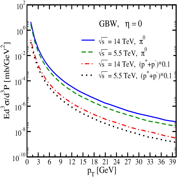
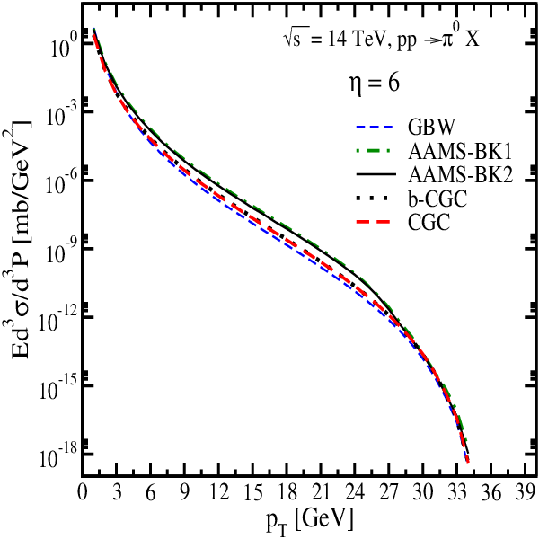
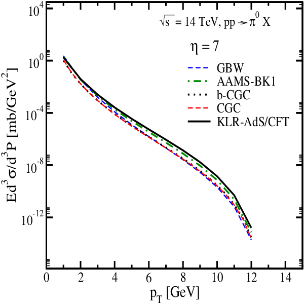

In Fig. 3, we show dipole model results obtained from the light-cone factorization in Eq. () for pion ( and proton () spectra at RHIC energy GeV and midrapidity. The experimental data are from PHENIX [53] and STAR [54]. For a compassion, we also show the results coming from an improved pQCD calculation performed in Ref. [55]. Notice that in the parton model results shown in Fig. 3 a fixed -factor was introduced in order to simulate higher order perturbative corrections while in the color dipole approach we do not introduce a -factor since the dipole-proton cross-section fitted to HERA incorporates all higher order radiations. Note that all the above-mentioned parametrizations for the color dipole cross-section have been fitted to DIS data at . This corresponds to GeV for RHIC energy at midrapidity (see Eq. (2)), so the PHENIX and STAR data plotted in Fig. 3 are not suited for a model test. It is seen from Fig. 3 that deviation of color dipole results from the experimental data starts at about GeV. At LHC energies and TeV for a large range of (even at ) we have , therefore we expect the color dipole prescription to be valid. In Fig. 4, we show the predictions of the GBW model for pion spectra in collisions for LHC energies TeV at midrapidity . The predictions for pion invariant cross-sections at various rapidities in collisions for LHC are given in Fig. 5. One can see from Fig. 5 that various dipole models presented in the previous section with explicit saturation give rather similar results (we will scrutinize this below). Note that the KLR-AdS/CFT model described in Sec. VI-C was fitted to the HERA data with and . Therefore it is only valid at very forward rapidities and low . As it is seen in the upper panel of Fig. 5, the two color dipole solutions of the BK equation for the GBW and MV initial conditions (AAMS-BK1,2) give very similar results and further on we will only consider one of them.
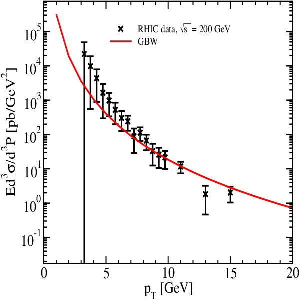
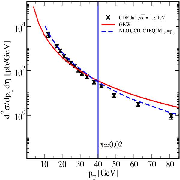

In Fig. 6, we show direct photon spectra obtained in our color-dipole approach Eq. (V), at the RHIC [58] ( GeV) and CDF ( TeV) energy [59, 57]. Again, we should warn that our results at high for lower energies like RHIC and CDF are less reliable since which is beyond the limit of applicability of the color-dipole light-cone factorization scheme. Nevertheless, the agreement of our results with available data for both hadron and photon production at RHIC and CDF energies is rather satisfactory for . As a comparison, in Fig. 6, we also show the NLO pQCD curve for CDF energy [56]. The predictions for direct photon spectra at LHC energies in collisions within various color-dipole models can be found in Ref. [23].
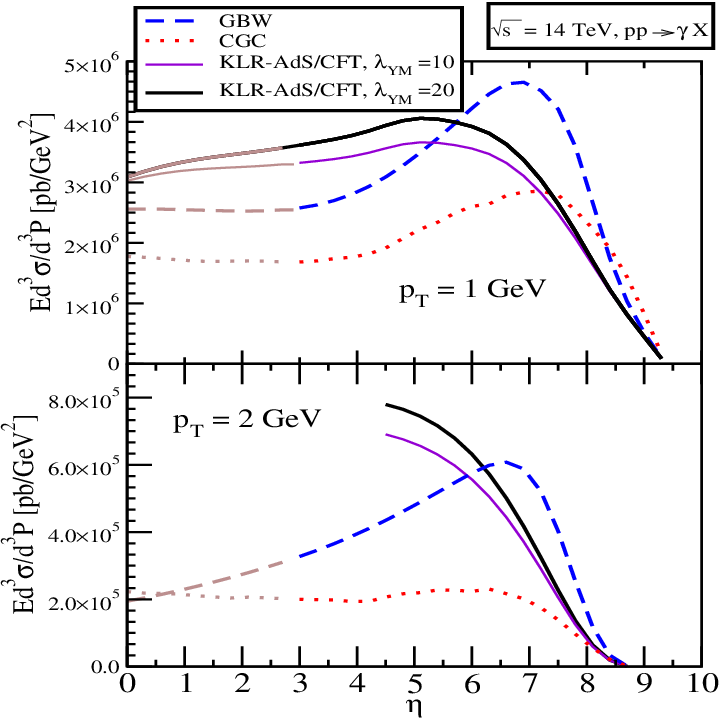
In Fig. 7, the differential cross-section of pion (top panel) and direct photon (lower panel) production at LHC are plotted versus rapidity at fixed transverse momenta and GeV within various color-dipole models. It is seen that the discrepancies among various saturation color dipole model results can be about a factor of at moderate rapidities. At the kinematic limit, i.e. at very forward rapidities and higher where the differential cross-section approaches zero, kinematic constraints limit the parton phase space and saturation effects become less important. This is seen in Fig. 7 where as we approach very forward rapidities at the kinematic limit, the discrepancies among various saturation models shrink, and the invariant cross-section identically approaches zero. Notice that for hadron production in the master Eq. (), the light-cone momentum fraction (where is the fragmentation fraction) enters the gluon radiation cross-section and therefore the color dipole cross-section, while in the case of direct photon production Eq. (V), we have . Therefore, the applicability of the KLR-AdS/CFT model which is valid for (and ), can be extended for direct photon production to lower rapidities compared to the case of hadrons. It is seen from Fig. 7 that for both hadron and photon production, away from the kinematic limit, at not very large and , a color-dipole model with larger saturation scale leads to a stronger peak at forward rapidity (having in mind that the saturation scale is a dynamical function of , see Fig. 2).

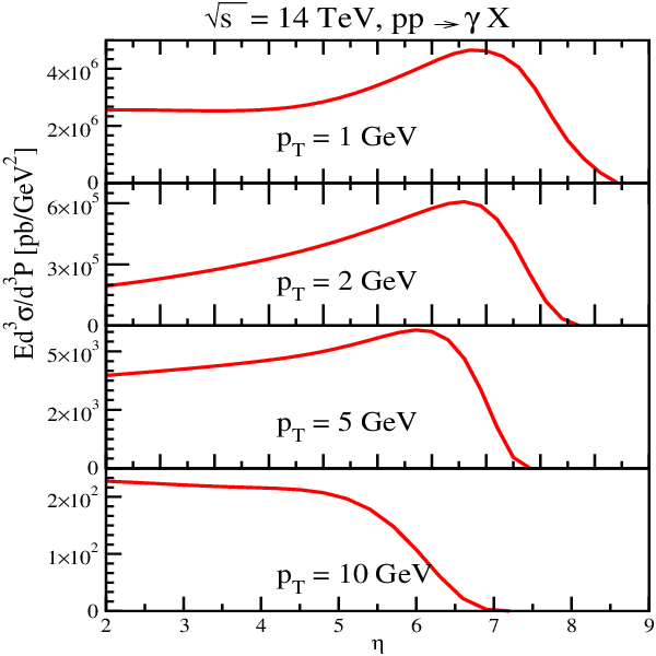
In Fig. 7, it is seen a peculiar enhancement of the photon production rate at forward rapidities. This feature is more obvious in Figs. 8 and 9 where we plot the differential cross-section of pion and direct photon production at LHC as a function of rapidity at fixed transverse momenta and GeV within the GBW model. It is obvious that the invariant cross-sections have a peak at forward rapidity. However, compared to pions, the peak of the differential cross-section for direct photon production persists at larger . It seems that several mechanisms are at work here in different kinematic regions. Looking again at Fig. 7 it is obvious that in the case of direct photons when the saturation scale is smaller (the CGC model) at higher transverse momentum GeV, the peak disappears and will be replaced by a plateau. However, in the case of pion production, the peak is less pronounced even in the presence of a large saturation scale, see Figs. 7 and 8. Moreover, photons are radiated by the electric current of the projectile quarks, which mostly stay in the fragmentation region of the beam, and tend to form a peak at forward rapidities. However, at very large and , the kinematic limit pushes photon radiation to more central rapidities and the peak at forward rapidities will be replaced by a kind of plateau at central rapidities. At the same time, gluons are radiated via nonabelian mechanisms by the color current across the whole rapidity interval and tend to form a plateau at midrapidity.
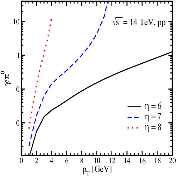
Another interesting difference between direct photon and hadron production is that direct photon production extends to higher rapidities for a fixed , see Figs. 8 and 9. This is more obvious in Fig. 10 where we show the photon/pion ratio as a function of at various rapidities within the GBW model and collisions. The ratio can be as big as at very forward rapidities at LHC energy. Note that suppression of hadrons at very forward rapidity also ensures significant suppression of radiative decays of those hadrons. Therefore, direct photon production at forward rapidities should be a rather clean signal.
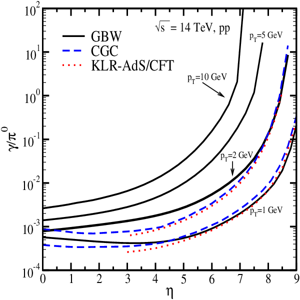
In Fig. 11, we show the ratio of photon/pion production as a function of rapidity in collision at LHC for various fixed within different saturation models. Direct photons can only be radiated from quarks, while hadrons can be produced by both gluons and quarks. At the LHC energy at midrapidity gluons dominate. Therefore the photon/pion ratio is significantly reduced toward midrapidity. However, at very forward rapidity, valence quarks become important and the photon/pion ratio rises. Moreover, at high again valence quarks becomes important and we have a sharp rise of the photon/pion ratio, see Fig. 11. A similar behavior has also been reported in a different approach [60].
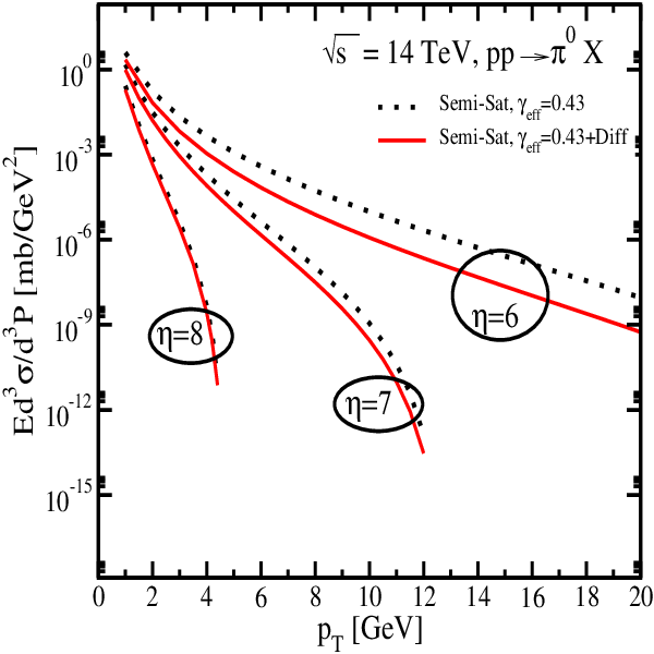
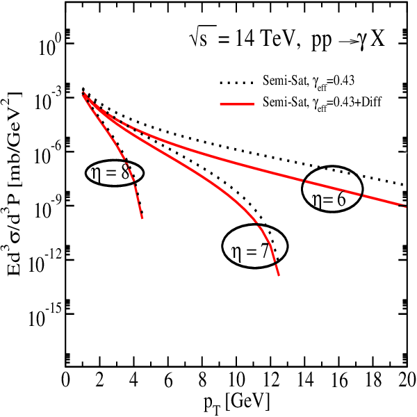
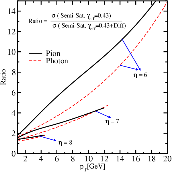
In order to understand the relative importance of saturation effects at various rapidities, we employ the Semi-Sat model. In Fig. 12 we show, the differential cross-section of pion and photon production at LHC, calculated once with diffusion term and once without, i.e. . We recall that the Semi-Sat model in the presence of the diffusion term describes -data at HERA, see Sec.VI-C. In Fig. 12 we show that at forward rapidities, the diffusion term in the anomalous dimension is not important, since it gives similar results as with a fixed . The preferred value of anomalous dimension at very forward rapidities is close to the one predicted from the BK equation [43]. This is more obvious in Fig. 13 where we show the ratio of the two cross-sections for both pions and direct photons. It is well known that the saturation effects start being essential when the anomalous dimension reaches the value which is the case for forward rapidities (see Refs. [1, 61, 40]). This indicates that direct photon and hadron production at different rapidities at LHC are rather sensitive to saturation.
VIII Cronin effect and nuclear modification factor
The nuclear modification (Cronin) factor is defined as ratio of to cross-sections normalized to the average number of binary nucleon collisions,
| (38) |
, the average number of geometrical binary collisions, is calculated according to the Glauber model [62] for different centralities.
Two very different mechanisms have been proposed to explain Cronin enhancement (or suppression) in collisions: a) initial-state effects [63, 26, 7, 64, 65] due to a broadening of the parton transverse momentum in the initial-state. Here the fragmentation of hard partons is assumed to occur outside the cold medium. b) final-state effects [8] due to the recombination of soft and shower partons in the final-state.
In our approach, the Cronin effect originates from initial-state broadening of the transverse momentum of a projectile parton interacting coherently with a nuclear medium. The invariant cross-section of hadron and direct photon production in collisions can be obtained via the light-cone color-dipole factorization scheme defined in Eqs. (,V).
VIII.1 Gluon shadowing
In the infinite momentum frame, the gluon clouds of nucleons which have the same impact parameter overlap at small Bjorken-x in the longitudinal direction. This allows gluons which originate from different nucleons to fuse, corresponding to a nonlinear term in the evolution equation which suppresses gluon production, and a precocious onset of the saturation effects for heavy nuclei. This is called gluon shadowing. The same effect, looks different in the rest frame of the nucleus, the gluon shadowing correction can be calculated as Landau-Pomeranchuk effect, namely the suppression of bremsstrahlung by interference of radiation from different scattering centers. This mechanism requires a sufficiently long coherence time for radiation, a condition equivalent to requiring a small Bjorken-x in the parton model.
The question if gluon shadowing is an intrinsically leading twist effect [66] or is suppressed by power of and is due to higher twist/high parton density effects [1, 2] is still debatable. There has been several shadowing models which consider only leading twist shadowing, e. g., including shadowing effects in the non-perturbative initial conditions which are then evolved with leading twist DGLAP equations [67]. Modifications of this leading twist picture to include Mueller-Qiu type non-linear contributions has been studied in Ref. [68].
In our approach, nuclear shadowing for gluons is calculated from shadowing of the Fock component of a longitudinally polarized photon. Unlike transverse photons, all dipoles from longitudinal photons have size and the double-scattering term vanishes like . The leading-twist contribution for the shadowing of the longitudinal photons arises, therefore, from the Fock component. While the separation is of order , the gluon can propagate relatively far from the -pair. After gluon radiation is in a color octet state, consequently the system appears as dipole. The shadowing correction to the longitudinal cross-section is then directly related to gluon shadowing. The gluon shadowing ratio is defined as the ratio of the gluon densities in a nucleus and a nucleon [10, 69]:
| (39) |
where is the inelastic correction to the longitudinal photoabsorption cross-section due to the creation of a Fock component. The details for the calculation of the suppression factor can be found in Refs. [10, 69, 70]. For a proton target, we have by construction.
At high energy the dipole cross-section is also subject to the multi-pomeron fusion effects in a nuclear medium. These effects are missed in the eikonal formulas Eqs. (,15,16,17) where the variation of the transverse size of the Fock component while propagating and interacting with a medium was not taken into account. Consequently higher Fock components were summed up without incorporating gluon shadowing. One should note that the multiple parton interactions that lead to gluon shadowing are also the source of gluon saturation. In order to avoid double counting, we calculate the nuclear shadowing effect within the same color-dipole formulation. The authors of Refs. [10, 69] have performed such a calculation by numerically solving the dipole evolution equations in a medium by light-cone Green function techniques and confronted DIS data for nuclei. Following Refs. [26, 7, 10, 69, 70] one can effectively incorporate gluon shadowing due to the nuclear medium by modifying the cross-section of the dipole interacting with a nucleus target at impact parameter by the following replacement
| (40) |
in the exponent of Eqs. (,15,16,17). Therefore, by means of and the dipole cross-section on a nucleon target, one can effectively define the dipole cross-section for a nucleus target by using Glauber theory, i.e. via simple eikonalization of the -nucleon cross-section modified by the suppression factor . In this way, we relate the nuclear gluon shadowing to the gluon saturation which can be then read off from the constructed dipole-nucleus forward amplitude. However, the question if the parton saturation provides a precise microscopic understanding of shadowing is an open question and out of scope of this paper. One should also note that although the shadowing factor improves the eikonal approximation, it is not apparently a solution of the non-linear BK evolution equation.
In the CGC picture, the dipole-nucleus amplitude has the same functional form as the dipole-nucleon amplitude. The only difference is the saturation scale. The -dependence of dipole-nucleus amplitude enters through the saturation scale where is the effective mass number of the nucleus in a given centrality and depends on the impact parameter. Our approach is different but is not in contradiction with the CGC picture at the saturation boundary. In order to see this, let us assume that in spirit of the CGC picture one can write the forward dipole-nucleus amplitude in the following form (we use the GBW form for simplicity),
| (41) |
By comparing the above equation with Eq. (15) and assuming that there is no correlation between dipole amplitude and the nuclear thickness, one can immediately read off the effective saturation scale in Eq. (15) close to the saturation boundary,
| (42) | |||||
| (43) |
where in the second line we rely on the small- approximation of the dipole cross-section (valid for a large ) and use the fact that at since . Therefore, the square of saturation scale in our approach is approximately proportional to since , in agreement with the basic idea of saturation and the CGC picture [1, 2, 5, 71]. Let us repeat the above steps in a slightly different way. The dipole-nucleon cross-section at small dipole size can be related to the gluon distribution in the nucleon [72],
| (44) |
By plugging the above expression into Eq. (42) we obtain,
| (45) |
where the typical value of dipole size can be related to the saturation scale . This is remarkably similar to the saturation scale proposed by by Kharzeev, Levin and Nardi (KLN model) [73],
| (46) |
where for collisions the density of participants is . Note that Eq. (46) gives the saturation scale for gluons and it is different from the saturation scale for quarks Eq. (45) by a Casimir factor . The KLN model Eq. (46) gives a good description of hadron multiplicities in heavy ion collisions at RHIC [73]. The main difference between our model Eq. (45) and the KLN model Eq. (46) is the shadowing factor which takes into account approximately multi-pomeron fusion effects in a nuclear medium beyond the eikonal approximation, see also Ref. [74].
In the limit of strong shadowing at very small , the gluon ratio Eq. (39) has a simple form where is the effective cross-section responsible for shadowing and is the nuclear radius. Therefore, in our approach, deep inside saturation region, we have and consequently the saturation scale becomes independent of . This behavior has been also predicted based on more sophisticated models indicating that the parton wave functions of different nuclei become universal at high energies limit [75, 76]. Nevertheless, we expect that our approach based on an improved eikonal approximation will not be reliable at such an extreme limit and we use our formulation only at midrapidity for collisions at RHIC and LHC energies.
As we argued above, in principle one may construct the dipole-nucleus amplitude via the dipole-nucleon amplitude supplemented with the -dependent saturation scale. However, it is not a priori obvious whether such a model with parameters fitted to the available DIS data on proton target is also able to describe the DIS data on nucleus target at small- without having to change the parameters of the model (the issue of sensitivity of the model parameters obtained from a fit to data in analysis), see Ref. [77]. In our approach we use the same dipole-nucleus cross-section which gives a good description of HERA data to calculate the cross-section in reactions. We stress again that the shadowing factor is not a free parameter in our formalism but it is calculated via Eq. (39). Such a shadowing factor is needed in order to describe the DIS data off nuclei [26, 7, 10, 69, 70]. Therefore the suppression obtained as a result of the inclusion of the shadowing factor (which depends on kinematics) is not arbitrary.
VIII.2 Numerical results for collisions
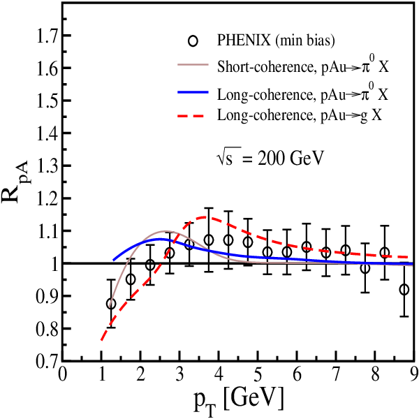
For the calculation of cross-sections for collisions, we use the same PDFs and FFs as for collisions. Furthermore, we use a Woods-Saxon nuclear profile for . We again stress that similar to the calculation for collisions, here again we have no free parameters to adjust. In Fig. 14, we show for production at RHIC in minimum bias proton-gold collisions. The experimental data in Fig. 14 are from PHENIX [53]. As we already mentioned, for RHIC energy at midrapidity and moderate , the coherence length defined via Eq. (2) is about fm which is comparable to the nuclear radius. Therefore, we are in the transition region between the regimes of long and short coherence length. Calculations in such a region are most complicated. In Fig. 14, we show the theoretical curves calculated in the two extreme cases of short- and long-coherence length. The curve for the short-coherence length in Fig. 14 is based on an improved pQCD calculation taken from Ref. [55]. We used the AKK08 for FFs, MSTW2008 for PDFs and the GBW model for the color dipole cross-section. One should also note that the color dipole cross-section is fitted to the DIS data for . Therefore, our results at high for RHIC are less reliable. At RHIC and LHC energies at midrapidity, gluons are mostly responsible for pion production. We also show in Fig. 14 the Cronin ratio for gluon production in proton-gold collisions. It is seen that fragmentation processes distort the gluonic Cronin enhancement and shift the Cronin peak to a lower .
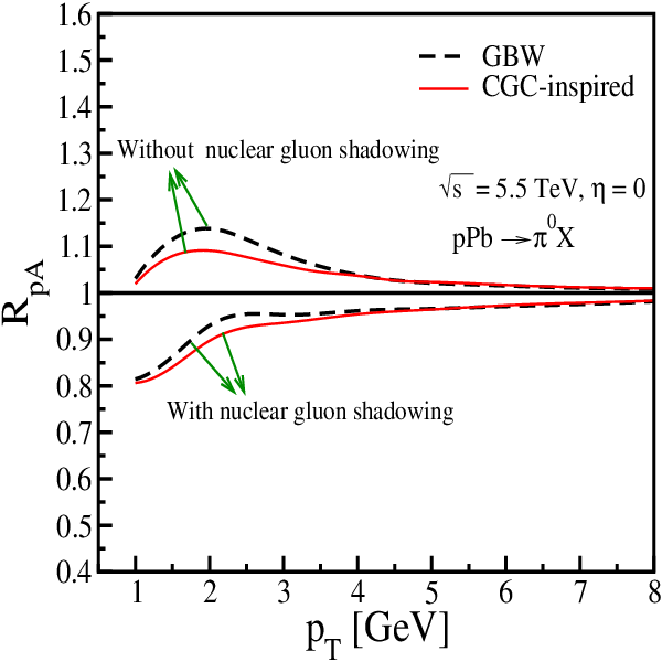
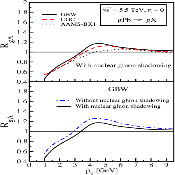
In Fig. 15, we show our prediction for the nuclear modification factor for production at LHC at midrapidity in minimum bias collisions within two very different saturation models, namely GBW and CGC. We also show the effect of nuclear gluon shadowing. It is seen that the Cronin enhancement will be replaced with moderate suppression in all saturation models considered in this paper due to nuclear gluon shadowing. It is obvious that a -proton dipole model with a bigger saturation scale leads to a larger Cronin enhancement and works against the nuclear shadowing suppression. This effect has also been shown in Ref. [78]. Note that the source of both saturation and shadowing is parton multiple interaction. However, a larger saturation scale leads to a stronger broadening of transverse momentum of the projectile partons and consequently it works against shadowing. This is more obvious in Fig. (16) (uppor panel) where we plotted the Cronin ratio for gluons production at the LHC energy within various saturation color dipole models. In Fig. (16) (lower panel) we show effect of nuclear gluon shadowing within the GBW color dipole model. It is seen that both shadowing and saturation effects are important at LHC in collisions and give rise to a rather sizable effect in the nuclear modification factor .
In Fig. 17, We show our prediction for the nuclear modification factor for direct photon production at LHC at midrapidity in minimum bias collisions for two models with different saturation scale. In order to demonstrate the importance of nuclear gluon shadowing effects, we have also plotted the curves without nuclear gluon shadowing. In comparison to pion production, the Cronin enhancement for direct photon production seems stronger and survives within the GBW color-dipole model which has a bigger saturation scale, even after the inclusion of nuclear gluon shadowing suppression effects. Similar to pion production, the Cronin enhancement for direct photon production is bigger in a model with a larger saturation scale. Within the CGC model both pion and direct photon enhancement at RHIC will be replaced by suppression at LHC.

In a similar approach, Kopeliovich et al. [26] have shown that the Cronin enhancement will survive at LHC at midrapidity though reduced compared to RHIC. Here, our finding is different. This is due to the fact that we improved the earlier calculation in several ways including: using updated PDFs, FFs and color-dipole cross-sections, incorporating gluon radiation from the quark projectile (i.e. , see Eq. ()), using recently upgraded shadowing suppression factor [70] and using a running strong coupling. Nevertheless, in both approaches the Cronin ratio is still very small, less than at midrapidity at LHC. Kharzeev et al. [64] have shown a marked suppression for pions at midrapidity at LHC in collisions based on the CGC scenario. This suppression is stronger than our prediction. Certainly, LHC data should be able to decide between the different approaches and scenarios.
Notice that our prescription for both hadron and photon production in collisions is less reliable at very large and also forward rapidities. This is due to the fact that at large (i.e. ) one should properly incorporate energy conservation since it puts an important constraint on particle production [7] . Nevertheless, we expect this effect to be negligible in our kinematical region of interest. Note also that the energy loss effects are subject to -scaling and less important for high-energy collisions at moderate , although it might be important at lower energies [7, 26]. A more detailed study of the Cronin effect for direct-photon production at RHIC and LHC at forward rapidities and high will be presented elsewhere [79].
IX Conclusions and outlook
In this paper, we investigated pion and direct photon production within a unified color-dipole approach at high-energy and collisions and provided various predictions for the upcoming LHC experiments. The results of this paper can be summarized as follows:
- •
Both hadron and direct photon production strongly depend on the value of the anomalous dimension and are sensitive to gluon saturation effects at forward rapidities at LHC ( TeV). The difference between various saturation model predictions can be about a factor . Note that all saturation models employed here are fitted to HERA data.
- •
We showed that the ratio of photon/pion production at LHC ( TeV) at very forward rapidities in collisions can be as big as . Therefore, direct photons at very forward rapidities should be a rather clean observable and provide a sensitive probe for saturation effects and small-x physics in general.
- •
We showed that the rapidity distribution of pions and direct photons exhibit some peculiar enhancement at forward rapidities which is more pronounced in the case of photon production. This peak is enhanced in models with a larger saturation scale at lower .
- •
We investigated the relationship between saturation and shadowing effects in collisions at LHC for both direct photon and hadron production. We studied the role of initial-state broadening of the transverse momentum distribution of a projectile parton propagating and interacting coherently with a nuclear medium. We showed that a larger saturation scale leads to a stronger transverse momentum broadening of the projectile partons and consequently works against the nuclear gluon shadowing suppression effects. Our results show that the nuclear modification factor at LHC is sensitive to both saturation and nuclear shadowing effects and it seems that a subtle cancellation between these two effects leads to a rather small Cronin ratio . We showed that the and direct photon Cronin ratio at the LHC is less than within the CGC color dipole model. However, in the case of direct photon production in collisions, the Cronin enhancement can survive at the LHC energy within the GBW color-dipole model which has a larger saturation scale.
Acknowledgements.
We would like to thank Javier Albacete, Boris Kopeliovich, Genya Levin, Marco Stratmann and Heribert Weigert for useful discussions. We are thankful to Yuri Kovchegov for useful communication in connection with Ref. [21]. A.R. acknowledges the financial support from the Alexander von Humboldt foundation, BMBF (Germany), Conicyt Programa Bicentenario PSD-91-2006, Fondecyt grants 1090312 (Chile).References
- [1] L. V. Gribov, E. M. Levin, and M. G. Ryskin, Phys. Rept. 100, 1 (1983).
- [2] A. H. Mueller and J.-W. Qiu, Nucl. Phys. B268, 427 (1986); L. D. McLerran and R. Venugopalan, Phys. Rev. D50, 2225 (1994); L. D. McLerran and R. Venugopalan,Phys. Rev. D49, 3352 (1994) ; L. D. McLerran and R. Venugopalan, Phys. Rev. D49, 2233 (1994) ; Y. V. Kovchegov, Phys. Rev. D54, 5463 (1996) ; Y. V. Kovchegov, Phys. Rev. D55, 5445 (1997); J. Jalilian-Marian, A. Kovner, L. D. McLerran, and H. Weigert, Phys. Rev. D55, 5414 (1997).
- [3] Y. V. Kovchegov, Phys. Rev. D60, 034008 (1999) ; Y. V. Kovchegov, Phys. Rev. D61, 074018 (2000) ; I. Balitsky, Nucl. Phys. B463, 99 (1996); I. Balitsky, hep-ph/9706411; I. Balitsky, Phys. Rev. D60, 014020 (1999).
- [4] J. Jalilian-Marian, A. Kovner, A. Leonidov, and H. Weigert, Nucl. Phys. B504, 415 (1997); J. Jalilian-Marian, A. Kovner, A. Leonidov, and H. Weigert, Phys. Rev. D59, 014014 (1998) ; J. Jalilian-Marian, A. Kovner, and H. Weigert, Phys. Rev. D59, 014015 (1998); J. Jalilian-Marian, A. Kovner, A. Leonidov, and H. Weigert, Phys. Rev. D59, 034007 (1999); A. Kovner, J. G. Milhano, and H. Weigert, Phys. Rev. D62, 114005 (2000); H. Weigert, Nucl. Phys. A703, 823 (2002); E. Iancu, A. Leonidov, and L. D. McLerran, Nucl. Phys. A692, 583 (2001); E. Ferreiro, E. Iancu, A. Leonidov, and L. McLerran, Nucl. Phys. A703, 489 (2002).
- [5] E. Iancu and R. Venugopalan, hep-ph/0303204; H. Weigert, Prog. Part. Nucl. Phys. 55, 461 (2005); J. Jalilian-Marian and Y. V. Kovchegov, Prog. Part. Nucl. Phys. 56, 104 (2006).
- [6] I. Arsene et al. [BRAHMS Collaboration], nucl-ex/0410020; B. B. Back et al., [PHOBOS Collaboration], nucl-ex/0410022; K. Adcox et al. [PHENIX Collaboration], nucl-ex/0410003; J. Adams et al. [STAR Collaboration], nucl-ex/0501009.
- [7] B. Z. Kopeliovich, J. Nemchik, I. K. Potashnikova, M. B. Johnson, I. Schmidt, Phys. Rev. C72, 054606 (2005); J. Nemchik, V. Petracek, I. K. Potashnikova and M. Sumbera, Phys. Rev. C78, 025213 (2008).
- [8] R. C. Hwa and C. B. Yang, Phys. Rev. Lett. 93, 082302 (2004); R. C. Hwa and C. B. Yang, Phys. Rev. C70, 037901 (2004). R. C. Hwa, C. B. Yang and R. J. Fries, Phys. Rev. C71, 024902 (2005).
- [9] D. Kharzeev, Y. V. Kovchegov and K. Tuchin, Phys. Lett. B599, 23 (2004).
- [10] B. Z. Kopeliovich, A. Schäfer and A. V. Tarasov, Phys. Rev. D62, 054022 (2000).
- [11] B. Z. Kopeliovich, I. K. Potashnikova, B. Povh and I. Schmidt, Phys. Rev. D76, 094020 (2007).
- [12] B. Z. Kopeliovich, A. Schäfer and A. V. Tarasov, Phys. Rev. C59, 1609 (1999).
- [13] N. N. Nikolaev and B. G. Zakharov, JETP 78, 598 (1994); Z. Phys. C64, 631 (1994).
- [14] High-Energy Particle Diffraction , V. Barone and E. Predazzi (Springer, Berlin, Heidelberg, 2002).
- [15] M. D. Elia, A. Di Giacomo and E. Meggiolaro, Phys. Lett. B408, 315 (1997).
- [16] E. V. Shuryak and I. Zahed, Phys. Rev. D69, 014011 (2004).
- [17] B.Z. Kopeliovich, H. J. Pirner, A. H. Rezaeian and I. Schmidt, Phys. Rev. D77, 034011 (2008)[arXiv:0711.3010]; B. Z. Kopeliovich, A. H. Rezaeian, I. Schmidt, Phys. Rev. D78, 114009 (2008)[arXiv:0809.4327]; Nucl. Phys. A807, 61 (2008)[arXiv:0712.2829]; arXiv:0804.2283.
- [18] J. P. Blaizot, F. Gelis and R. Venugopalan, Nucl. Phys. A743, 57 (2004); C. Marquet, Nucl. Phys. A796, 41 (2007).
- [19] J. Jalian-Marian and Y. Kovchegov, Phys. Rev. D70, 114017 (2004).
- [20] Y. V. Kovchegov and A. H. Mueller, Nucl. Phys. B529, 451 (1998).
- [21] Y. V. Kovchegov and K. Tuchin, Phys. Rev. D65, 074026 (2002).
- [22] B. Z. Kopeliovich, A. H. Rezaeian, H. J. Pirner and I. Schmidt, Phys. Lett. B653, 210 (2007)[arXiv:0704.0642].
- [23] B. Z. Kopeliovich, E. Levin, A. H. Rezaeian, I. Schmidt, Phys. Lett. B675, 190 (2009)[arXiv:0902.4287]; A. H. Rezaeian et al., arXiv:0707.2040; N. Armesto et al., J. Phys. G35, 054001 (2008)[arXiv:0711.0974].
- [24] B. Z. Kopeliovich, J. Raufeisen and A. V. Tarasov, Phys. Lett. B503, 91 (2001) [arXiv:hep-ph/0012035].
- [25] J. Raufeisen, J.-C. Peng and G.C. Nayak, Phys. Rev. D66, 034024 (2002); J. Raufeisen, PhD-thesis, arXiv:hep-ph/0009358.
- [26] B. Z. Kopeliovich, J. Nemchik, A. Schäfer and A. V. Tarasov, Phys. Rev. Lett. 88, 232303 (2002).
- [27] B. Z. Kopeliovich, A. H. Rezaeian, Int. J. Mod. Phys. E18, 1629 (2009)[arXiv:0811.2024] and references therein.
- [28] A. Dumitru, A. Hayashigaki and J. Jalilian-Marian, Nucl. Phys. A770, 57 (2006) [arXiv:hep-ph/0512129], Nucl. Phys. A765, 464 (2006) [arXiv:hep-ph/0506308].
- [29] K. Golec-Biernat and M. Wüsthoff, Phys. Rev. D60, 114023 (1999).
- [30] E. A. Kuraev, L. N. Lipatov, and V. S. Fadin, Sov. Phys. JETP 45, 199 (1977); Y. Y. Balitsky and L. N. Lipatov Sov. J. Nucl. Phys. 28, 822 (1978).
- [31] V. S. Fadin and L. N. Lipatov, Phys. Lett. B429, 127 (1998); M. Ciafaloni and G. Camici, Phys. Lett. B430, 349 (1998); I. Balitsky and G. A. Chirilli, Phys. Rev. D77, 014019 (2008); D. A. Ross, Phys. Lett. B431, 161 (1998); Y. V. Kovchegov and A. H. Mueller, Phys. Lett. B439, 428 (1998).
- [32] J. L. Albacete, Phys. Rev. Lett. 99, 262301 (2007); M. Ciafaloni and G. Camici, Phys. Lett. B430, 349 (1998); I. Balitsky and G. A. Chirilli, Phys. Rev. D77, 014019 (2008); D. A. Ross, Phys. Lett. B431, 161 (1998); Y. V. Kovchegov and A. H. Mueller, Phys. Lett. B439, 428 (1998); M. Ciafaloni, D. Colferai, and G. P. Salam, Phys. Rev. D60, 114036 (1999).
- [33] I. I. Balitsky, Phys. Rev. D75, 014001 (2007); Y. Kovchegov and H. Weigert, Nucl. Phys. A784, 188 (2007); E. Gardi, J. Kuokkanen, K. Rummukainen, and H. Weigert, Nucl. Phys. A784, 282 (2007); J. L. Albacete and Y. V. Kovchegov, Phys. Rev. D75, 125021 (2007).
- [34] J. L. Albacete, N. Armesto, J. G. Milhano and C. A. Salgado, arXiv:0902.1112.
- [35] G. Watt and H. Kowalski, Phys. Rev. D78, 014016 (2008).
- [36] H. Kowalski, L. Motyka and G. Watt, Phys. Rev. D74, 074016 (2006).
- [37] H. Kowalski and D. Teaney, Phys. Rev. D68, 114005 (2003).
- [38] E. Iancu, K. Itakura, and L. McLerran, Nucl. Phys. A708, 327 (2002).
- [39] D. N. Triantafyllopoulos, Nucl. Phys. B648, 293 (2003).
- [40] A. H. Mueller and D.N. Triantafyllopoulos, Nucl. Phys. B640, 331 (2002); D. N. Triantafyllopoulos, Nucl. Phys. B648, 293 (2003).
- [41] E. Iancu, K. Itakura and S. Munier, Phys. Lett. B590, 199 (2004).
- [42] G. Watt and H. Kowalski, Phys. Rev. D78, 014016 (2008).
- [43] D. Boer, A. Utermann and E. Wessels, Phys. Rev. D75, 094022 (2007)[arXiv:hep-ph/0701219].
- [44] J. M. Maldacena, Adv. Theor. Math. Phys. 2, 231 (1998); S. S. Gubser, I. R. Klebanov, and A. M. Polyakov, Phys. Lett. B428, 105 (1998); E. Witten, Adv. Theor. Math. Phys. 2, 253 (1998); O. Aharony, S. S. Gubser, J. M. Maldacena, H. Ooguri, and Y. Oz, Phys. Rept. 323, 183 (2000).
- [45] Y. V. Kovchegov, Z. Lu and A. H. Rezaeian, Phys. Rev. D80, 074023 (2009) [arXiv:0906.4197].
- [46] A. M. Stasto, K. J. Golec-Biernat and J. Kwiecinski, Phys. Rev. Lett. 86, 596 (2001) [arXiv:hep-ph/0007192].
- [47] E. Levin and K. Tuchin, Nucl. Phys. B573, 833 (2000) [arXiv:hep-ph/9908317]; Nucl. Phys. A691, 779 (2001)[arXiv:hep-ph/0012167].
- [48] E. Iancu, K. Itakura and L. McLerran, Nucl. Phys. A708, 327 (2002)[arXiv:hep-ph/0203137].
- [49] A. H. Mueller and D. N. Triantafyllopoulos, Nucl. Phys. B640, 331 (2002)[arXiv:hep-ph/0205167].
- [50] A. D. Martin, W. J. Stirling, R. S. Thorne, G. Watt, arXiv:0901.0002.
- [51] S. Albino, B. A. Kniehl and G. Kramer, Nucl. Phys. B803, 42 (2008).
- [52] A. Vogt, Comput. Phys. Commun. 170, 65 (2005).
- [53] S. S. Adler et al. [PHENIX Collaboration], Phys. Rev. Lett. 98, 172302 (2007).
- [54] J. Adams et al. [STAR Collaboration], Phys. Lett. B637, 161 (2006).
- [55] A. H. Rezaeian and Z. Lu, Nucl. Phys. A826, 198 (2009)[arXiv:0810.4942].
- [56] M. Glück, L. E. Gordon, E. Reya and W. Vogelsang, Phys. Rev. Lett. 73, 388 (1994).
- [57] CDF Collaboration, Phys. Rev. D70, 074008 (2004).
- [58] PHENIX Collaboration, Phys. Rev .Lett. 98, 012002 (2007).
- [59] CDF Collaboration, Phys. Rev. Lett. 73, 2662 (1994); 74,1891 (1995).
- [60] J. Jalilian-Marian, Nucl. Phys. A806, 305 (2008); S. Jeon, J. Jalilian-Marian and I. Sarcevic, Nucl. Phys. A715, 795 (2003).
- [61] J. Bartels and E. Levin, Nucl. Phys. B387, 617 (1992); S. Munier and R. B. Peschanski, Phys. Rev. D69, 034008 (2004)[arXiv:hep-ph/0310357]; Phys. Rev. Lett. 91, 232001 (2003)[arXiv:hep-ph/0309177].
- [62] R. J. Glauber and G. Matthiae, Nucl. Phys. B21, 135 (1970); K. J. Eskola, K. Kajantie, J. Lindfors Nucl. Phys. B323, 37 (1989).
- [63] J. W. Cronin et al., Phys. Rev. D11, 3105 (1975); X-N. Wang, Phys. Rev. C61, 064910 (2000); G. Papp, P. Levai and G. Fai, Phys. Rev. C61, 021902 (2000); A. Accardi and M. Gyulassy, Phys. Lett. B586, 244 (2004); E. Cattaruzza, D. Treleani, Phys. Rev. D69, 094006 (2004).
- [64] D. Kharzeev, Y. V. Kovchegov and K. Tuchin, Phys. Lett. B599, 23 (2004).
- [65] J. Jalilian-Marian, Y. Nara and R. Venugopalan, Phys. Lett. B577, 54 (2003); J. P. Blaizot, F. Gelis and R. Venugopalan, Nucl. Phys. A743, 13 (2004); D. Kharzeev, Yu. K., K. Tuchin, Phys.Rev. D68, 094013 (2003); Albacete, Armesto, Kovner, Salgado and Wiedemann, Phys. Rev. Lett. 92, 082001 (2004); E. Iancu, K. Itakura and D. N. Triantafyllopoulos, Nucl. Phys. A742,182 (2004); J. Jalilian-Marian, Nucl. Phys. A748, 664 (2005).
- [66] L. L. Frankfurt and M. I. Strikman, Phys. Rept. 160, 235 (1988).
- [67] See for example: K. J. Eskola, V. J. Kolhinen and C. A. Salgado, Eur. Phys. J. C9, 61 (1999); M. Hirai, S. Kumano and M. Miyama, Phys. Rev. D64, 034003 (2001).
- [68] K. J. Eskola, H. Honkanen, V. J. Kolhinen and C. A. Salgado, Phys. Lett. B532, 222 (2002).
- [69] B. Z. Kopeliovich, J. Raufeisen and A. V. Tarasov, Phys. Rev. C62, 035204 (2002); B. Z. Kopeliovich, J. Nemchik, A. Schäfer and A. V. Tarasov, Phys. Rev. C65 035201 (2002); J. Nemchik, Phys. Rev. C68, 035206 (2003).
- [70] B. Z. Kopeliovich, J. Nemchik, I. K. Potashnikova and I. Schmidt, J. Phys. G35, 115010 (2008)[arXiv:0805.4613].
- [71] A. H. Mueller, Nucl. Phys. B572, 227 (2000).
- [72] B. Blaettel, G. Baym, L. L. Frankfurt and M. Strikman, Phys. Rev. Lett. 70, 896 (1993).
- [73] D. Kharzeev and M. Nardi, Phys. Lett. B507, 121 (2001); D. Kharzeev and E. Levin, Phys. Lett. B523, 79 (2001); D. Kharzeev, E. Levin and M. Nardi, Nucl. Phys. A730, 448 (2004) [Erratum-ibid. A743, 329 (2004)].
- [74] A. L. Ayala, M. B. Gay Ducati and E. M. Levin, Nucl. Phys. B493, 305 (1997).
- [75] A. H. Mueller, Nucl. Phys. A724, 227 (2003).
- [76] D. Kharzeev, E. Levin and M. Nardi, Nucl. Phys. A747, 609 (2005).
- [77] V. P. Goncalves, M. S. Kugeratski, M. V. T. Machado and F. S. Navarra, Phys. Lett. B643, 273 (2006).
- [78] R. Baier, A. Kovner and U. A. Wiedemann, Phys. Rev. D68, 054009 (2003).
- [79] B.Z. Kopeliovich, J. Nemchik, A. H. Rezaeian and I. Schmidt, under preparation.