Early universe models from Noncommutative Geometry
Abstract.
We investigate cosmological predictions on the early universe based on the noncommutative geometry models of gravity coupled to matter. Using the renormalization group analysis for the Standard Model with right handed neutrinos and Majorana mass terms, which is the particle physics content of the most recent noncommutative geometry models, we analyze the behavior of the coefficients of the gravitational and cosmological terms in the Lagrangian derived from the asymptotic expansion of the spectral action functional of noncommutative geometry. We find emergent Hoyle-Narlikar and conformal gravity at the see-saw scales and a running effective gravitational constant, which affects the propagation of gravitational waves and the evaporation law of primordial black holes and provides Linde models of negative gravity in the early universe. The same renormalization group analysis also governs the running of the effective cosmological constant of the model. The model also provides a Higgs based slow-roll inflationary mechanism, for which one can explicitly compute the slow-roll parameters. The particle physics content allows for dark matter models based on sterile neutrinos with Majorana mass terms.
1. Introduction
The idea of using noncommutative geometry to give a conceptual mathematical formulation of the standard model of elementary particle physics dates back to the work of Connes [19]. It was shown more recently in [17] (see also [20], [4], and Chapter 1 of [22]) that the noncommutative geometry model of particle physics can be made compatible with right handed neutrinos and neutrino masses and that the full Lagrangian of the standard model with Majorana mass terms for the right handed neutrinos can be derived by a computation from a very simple input of an almost commutative space, the product of an ordinary spacetime manifold and a finite noncommutative space. The resulting physical Lagrangian in this noncommutative geometry model is obtained from the asymptotic expansion in the energy scale of a natural action functionals defined on noncommutative spaces, the spectral action, [14]. Among the most interesting features of these models of particle physics based on noncommutative geometry is the fact that the physical Lagrangian of the model is completely computed from a simple geometric input (the choice of a finite dimensional algebra), so that the physics is very tightly constrained by the underlying geometry. For reasons of space, we cannot include here any introductory material about Noncommutative Geometry, but we suggest the interested readers to look at the survey paper [23] for a user-friendly introduction based on examples, as well as the books [21] and [22] for a more complete treatment.
We focus here on the noncommutative geometry model obtained in [17]. The corresponding physical Lagrangian computed from the asymptotic expansion of the spectral action contains the full Standard Model Lagrangian with additional Majorana mass terms for right handed neutrinos, as well as gravitational and cosmological terms coupled to matter. The presence of these terms and their relation to the particle physics content of the model make this approach of interest to theoretical cosmology. The gravitational terms include the Einstein–Hilbert action with a cosmological term, a topological term related to the Euler characteristic of the spacetime manifold, and, additionally, a conformal gravity term with the Weyl curvature tensor and a conformal coupling of the Higgs field to gravity. Without these last two contributions essentially one would be dealing with the usual minimal coupling of the standard model to gravity, but the presence of an additional non-minimal conformal coupling has relevance to various cosmological models that have been the object of recent investigation, especially in the context of modified theories of gravity. Another important way in which this model differs from the minimal coupling of gravity and matter is the dependence of the coefficients of the gravitational terms upon the Yukawa parameters of the particle physics content of the model. This feature, which is our main focus of investigation in the present paper, is unique to these noncommutative geometry models and does not have an analog in other particle physics and cosmology models obtained from geometric settings such as string theories, extra dimensions, or brane worlds. Some conceptual similarities with these other approaches exist though, in the sense that in noncommutative geometry models one typically modifies ordinary spacetime by taking a product with a noncommutative space and this may be thought of as another possible way to enrich it with extra dimensions.
The fact that, as shown in [17], the model lives naturally at unification scale, means that in cosmological terms it provides us with early universe models, hence it is interesting in terms of possible inflationary mechanisms. Extrapolations to lower energies are possible using renormalization group analysis, though extensions to cosmological models of the more recent universe only become possible when non-perturbative effects in the spectral action are also taken into account. The main motivation for considering these noncommutative geometry models in a cosmological context is that the nontrivial dependence of the cosmological and gravitational parameters on the particle physics content is, as we mentioned above, significantly different from other physical models, hence likely to provide inflationary scenarios in the early universe that differ significantly from other models.
This paper is the first of a planned series dedicated to an investigation of the cosmological implication of the noncommutative geometry models in particle physics. In the present paper, we concentrate on a renormalization group analysis of the coefficients of the gravitational terms in the action. In fact, the asymptotic formula for the spectral action used in [17] shows that these coefficients are functions of certain parameters, which in turn depend on the data of the Yukawa parameters of the standard model with Majorana mass terms for right handed neutrinos. They also depend on three additional parameters of the model, one of which is fixed by a grand unification type condition on the coupling constants.
The Yukawa parameters run with the renormalization group equations of the particle physics model. In particular, since the noncommutative geometry model lives naturally at unification scale, one can input boundary conditions at that energy scale and follow the renormalization group equations towards lower energies and investigate the effect of this running on the gravitational part of the model. One expects that, when running towards lower energies, nonperturbative effects in the spectral action will progressively become non-negligible. This can limit the range of validity of this type of argument based on the asymptotic expansion alone, and on renormalization group analysis to cosmological models for the very early universe, that is, for sufficiently high energies where the asymptotic expansion holds. Any extrapolation to the modern universe would then have to take into account the full spectral action and not only its asymptotic form.
In the present paper we focus on early universe models and on the asymptotic form of the spectral action. For the renormalization analysis, we rely on a detailed study of the renormalization group equations (RGE) for the extension of the standard model with right handed neutrinos and Majorana mass terms carried out in [1], even though their choice of boundary conditions at unification is different from some of the boundary conditions assumed in [17]. The boundary conditions proposed in [1] are dictated by particle physics considerations, while some of the constraints considered in [17] came from analyzing particular geometries, such as the flat space case. For example, for simplicity the Majorana masses were assumed in [17] to be degenerate, all of them close to unification scale, while here we are mostly interested in the non-degenerate case, with three different see-saw scales between the electroweak and unification scales, which leads to a more interesting behavior of the gravitational terms in the model. We plan to return to a more general analysis of the RGE flow of [1] with a wider range of possible boundary conditions in followup work.
The RGE flow of [1] runs between a unification energy, taken there to be of the order of GeV, down to the electroweak scale of GeV. In terms of cosmological timeline, we are looking at the behavior of the model between the unification and the electroweak era. This means that, in terms of matter content, only the Higgs field and its coupling to gravity is relevant, so we mostly concentrate on the part of the Lagrangian of [17] that consists of these terms. Since this era of the early universe is believed to include the inflationary epoch, we look especially at different possible inflationary scenarios provided by this noncommutative geometry model.
Our main results in this first paper are to show that, using the information on the particle physics content, it is possible to obtain cosmological models of the early universe with variable gravitational and cosmological constant, hence providing a range of different mechanisms for inflation, realized by the running of the effective gravitational constant and by its coupling to the Higgs field, or by the running of the effective cosmological constant of the model, or by a combination of these. We also show phenomena where, near particular energy scales and for special geometries, the usual Einstein–Hilbert action ceases to be the dominant contribution and the model comes to be dominated, at certain scales, by conformal gravity and an emergent Hoyle–Narlikar cosmology. We discuss how the running of the gravitational parameters of the model influences the behavior of the evaporation of primordial black holes by Hawking radiation. While the type of effects that we see in this model, which depend on the presence of variable effective gravitational and cosmological constants, are qualitatively similar to scenarios of negative gravity in the early universe previously analyzed in theoretical cosmology ([5], [6], [11], [24], [25], [26], [35], [36], [37], [39], [40], [41], [43], [48]), the mechanism that produces these effects in the noncommutative geometry model is substantially different from those described in these earlier references, which makes the quantitative behavior also different and distinguishable from other models. In fact, most of the effects we investigate in this paper depend directly on the expression of the coefficients of the gravitational and bosonic terms in the asymptotic expansion of the spectral action in terms of the Yukawa parameters of the underlying particle physics model. This is a purely geometric property of this model and it comes directly from the presence of the “small extra dimensions” in the form of the zero dimensional (but K-theoretically six dimensional) finite noncommutative space in addition to the extended spacetime dimensions.
While the energy range where the renormalization group analysis applies limits the results based only on the perturbative expansion of the spectral action to early universe models, if some of the results obtained in this paper persist when non-perturbative effects in the spectral action become significant, they may provide possible dark energy and dark matter predictions. For instance, the behavior of the variable effective cosmological constant may lead to dark energy scenarios in the more recent universe. Moreover, we show that the particle physics content of the model is consistent with dark matter models based on right handed neutrinos with Majorana mass terms in [33], [44], [45]. In fact, the particle content is the same as in the MSM model with three active and three sterile neutrinos. What is needed in order to relate the model of [17] to these dark matter models is a choice of boundary conditions that makes it possible for at least one of the Majorana masses to descent to somewhere near the electroweak scale, hence providing sterile neutrinos with the characteristics required to give acceptable dark matter candidates (see the analysis in [33]). We will return to a closer analysis of dark energy and dark matter implications of the noncommutative geometry models in a planned continuation of this work.
In a related but different direction, recent work on some cosmological aspects of the model of [17] was also done in [38].
Acknowledgment. Part of this work was carried out during visits of the first author at the Mathematical Sciences Research Institute in Berkeley and at the Max Planck Institute for Mathematics in Bonn. The hospitality and support of both institutions is gratefully acknowledged.
2. The asymptotic formula for the spectral action and the gravitational parameters
We recall here briefly the main aspects of the noncommutative geometry model of particle physics derived in [17] that we need to use in the rest of the paper. We refer the reader to [17] and to Chapter 1 of [22] for a detailed treatment. The reader who wishes to skip this preliminary part can start directly with the asymptotic expansion of the spectral action recalled in §2.5, which is what we concentrate on in the rest of the paper, but we prefer to add a few words on the derivation of the model via noncommutative geometry for the sake of completeness.
2.1. Spectral triples and the spectral action functional
The particle physics models based on noncommutative geometry, both the original one of [19] and the new one of [17] that incorporates right handed neutrinos and neutrino mixing with Majorana mass terms, are based on the formalism of spectral triples. These were introduced by Connes [18] as an extension of the notion of Riemannian manifold to noncommutative geometry. The data defining a (real) spectral triple are summarized as follows.
- •
is an involutive algebra with unit. Requiring the algebra to be unital corresponds to working with compact manifolds. (Extensions of the notion of spectral triple to non-unital cases have also been developed.)
- •
is a separable Hilbert space endowed with a representation of the algebra by bounded linear operators.
- •
is a linear self-adjoint operator acting on . Except for finite dimensional cases, is in general not a bounded operator, hence it is only defined on a dense domain.
- •
has compact resolvent: is a compact operator.
- •
The commutators are bounded operators for all .
- •
The spectral triple is even if there is on a -grading satisfying and .
- •
The spectral triple has a real structure if there is an antilinear isomorphism with , , and , where the signs , , and determine the KO-dimension modulo of the spectral triple, according to by the table
n 0 1 2 3 4 5 6 7 1 1 -1 -1 -1 -1 1 1 1 -1 1 1 1 -1 1 1 1 -1 1 -1 - •
The Hilbert space has an -bimodule structure with respect to the action of defined by and satisfying the commutation condition for all and in .
- •
The operator satisfies the order one condition , for all .
Commutative geometries, which in this context means ordinary Riemannian manifolds, can be described as spectral triples: for a compact spin Riemannian manifold the associated spectral triple is given by the algebra of smooth functions, the Hilbert space of square integrable spinors, and the Dirac operator. The metric tensor can be recovered from these data. For an even dimensional manifold is the grading on the spinor bundle given by the usual chirality operator and the real structure is the charge conjugation operator. Examples of spectral triples associated to objects that are not manifolds include a wide range of geometries such as quantum groups, fractals, or noncommutative tori. As we recall in §2.2 below, the spectral triples involved in the particle physics models are of a very special form which is almost commutative, namely a product of an ordinary manifold with a small noncommutative space.
It was shown by Chamseddine and Connes [14] that there is a natural action functional on a spectral triple. This spectral action functional is defined as , where is a cutoff function and is the energy scale. There is an asymptotic formula for the spectral action, for large energy , of the form
| (2.1) |
where are the momenta of the function and the noncommutative integration is defined in terms of residues of zeta functions
| (2.2) |
The sum in (2.1) is over points in the dimension spectrum of the spectral triple, which is a refined notion of dimension for noncommutative spaces, consisting of the set of poles of the zeta functions (2.2).
2.2. The noncommutative space of the model
The main result of [17] is a complete derivation of the full standard model Lagrangian with additional right handed neutrino, lepton mixing matrix and Majorana mass terms, by a calculation starting from a very simple geometric input. The initial ansatz used in [17] is the choice of a finite dimensional algebra, the left-right symmetric algebra
| (2.3) |
where and are two copies of the real algebra of quaternions.
The representation is then naturally determined by taking the sum of all the inequivalent irreducible odd spin representations of , so that the only further input that one needs to specify is the number of generations. The (finite dimensional) Hilbert space is then given by copies of ,
The Hilbert space with the action splits as a sum of matter and antimatter sectors, and an orthogonal basis of gives all the fermions of the particle physics model
| (2.4) |
respectively giving the neutrinos, the charged leptons, the u/c/t quarks, and the d/s/b quarks in terms of the representation of . Here and are the basis of the representation of where the action of is, respectively, by or , and and are the actions of and , respectively, through the representation .
The -grading exchanges the left and right chirality of fermions and the real structure operator exchanges the matter and antimatter sectors and performs a complex conjugation. These properties of and suffice to determine the KO-dimension modulo of the resulting spectral triple and an interesting aspect is that, unlike in the earlier particle physics models based on noncommutative geometry, in this case the KO-dimension is modulo , although the metric dimension is zero.
The order one condition on the Dirac operator is seen in [17] as a coupled equation for a subalgebra and a Dirac operator and it is shown that there is a unique subalgebra of maximal dimension that allows for the order one condition to be satisfied. The algebra is of the form
| (2.5) |
where the first summand embeds diagonally into in , thus breaking the left-right symmetry. It is expected, though presently not known, that this symmetry breaking should be dynamical. This geometric argument identifying the maximal algebra on which the order one condition can be satisfied was later extended in [15] to more general ansatz algebras than , but with the same resulting .
2.3. Dirac operators: Yukawa parameters and Majorana masses
The selection of the subalgebra for the order one condition for the Dirac operator is what produces geometrically in this model the Majorana mass terms for right handed neutrinos. In fact, one has in [17] a complete classification of the possible Dirac operators on the noncommutative space compatible with and (see also [10] for a more general discussion of moduli spaces of Dirac operators for finite spectral triples). These are all of the form
with and , and with and respectively of the form
Here the -matrices involved in the expression of and are the Yukawa matrices that give Dirac masses and mixing angles. These are matrices in in the case of generations: is the Yukawa matrix for the charged leptons, for the neutrinos, for the d/s/b quarks, and for the u/c/t quarks. Moreover, the remaining term , with denoting transposition, gives the matrix in and is the symmetric matrix of the Majorana mass terms for right handed neutrinos.
Thus, the model of [17] has three active and three sterile neutrinos as in the MSM model, see [33], [44], [45], though in [17], unlike in the MSM model, it is assumed that the three sterile neutrinos all have masses well above the electroweak scale. The see-saw relation for neutrino masses is obtained in [17] geometrically from the fact that the restriction of the Dirac operator to the subspace of spanned by , , , is of the form
| (2.6) |
where is the neutrino mass matrix, see Lemma 1.225 of [22]. We return to discuss the relation of the model of [17] to the MSM model of [44], [45] and to other sterile neutrinos scenarios of [33] in the context of dark matter models in cosmology, see §5 below.
The spectral triple that determines the physical Lagrangian of the model through the asymptotic expansion of the spectral action is then the product geometry , of a 4-dimensional spacetime , identified with the spectral triple , and the finite noncommutative space defined by the spectral triple with of the form as above. The product is given by the cup product spectral triple with sign and real structure
- •
- •
- •
- •
and .
The action functional considered in [17] to obtain the physical Lagrangian has a bosonic and a fermionic part, where the bosonic part is given by the spectral action functional with inner fluctuations of the Dirac operator and the fermionic part by the pairing of the Dirac operator with fermions,
| (2.7) |
Here is the Dirac operator with inner fluctuations given by the gauge potentials of the form , for elements . The fermionic term should be seen as a pairing of classical fields , viewed as Grassman variables. This is a common way of treating Majorana spinors via Pfaffians, see §16.2 of [22].
While this fermionic part is very important for the particle physics content of the model, as it delivers all the fermionic terms in the Lagrangian of the Standard Model, for our purposes related to cosmological models of the early universe, it will suffice of concentrate only on the bosonic part of the action, given by the spectral action term , since during a good part of the cosmological period between the unification and the electroweak epoch the Higgs field is the matter content that will be mostly of relevance, [30].
2.4. Parameters of the model
As we have recalled above, the geometric parameters describing the possible choices of Dirac operators on the finite noncommutative space correspond to the Yukawa parameters of the particle physics model and the Majorana mass terms for the right handed neutrinos. We recall here some expressions of these parameters that appear in the asymptotic expansion of the spectral action and that we are going to analyze more in detail later in the paper. We define functions , , , , of the matrices , , , and of the Majorana masses in the following way:
| (2.8) |
In addition to these parameters, whose role we describe in §2.5, we see clearly from (2.1) that the asymptotic formula for the spectral action depends on parameters given by the momenta of the cutoff function in the spectral action. Since the noncommutative space here is of the simple form , the only contributions to the dimension spectrum, hence to the asymptotic formula for the spectral action come from three parameters , , , where and for
2.5. The asymptotic expansion of the spectral action
It was proved in [17] that the asymptotic formula (2.1) applied to the action functional of the product geometry gives a Lagrangian of the form
| (2.9) |
We see from this expansion how the coefficients of all the terms in this resulting action functional depend on the Yukawa and Majorana parameters through their combinations of the form , , , , defined as in (2.8), and from the three additional parameters , , .
The term of (2.9) with the Yang–Mills action for the gauge bosons,
contains the coupling constants , , of the three forces. As shown in [17], the standard normalization of these Yang–Mills terms gives the GUT relation between the three coupling constants and fixes the fact that this model lives naturally at a preferred energy scale given by the unification scale . The normalization of the Yang–Mills terms fixes the value of the parameter to depend on the common value at unification of the coupling constants: as shown in §4.5 and §5.1 of [17] one obtains
| (2.10) |
One also normalizes the kinetic term for the Higgs as in [17] by the change of variables to get .
The normalization of the Yang–Mills terms and of the kinetic term of the Higgs then gives, at unification scale, an action functional of the form
| (2.11) |
where the coefficients are now
| (2.12) |
again as a function of the Yukawa and Majorana parameters through the coefficients , , , , of (2.8), and of the two remaining free parameters of the model, and , after the value of has been fixed by the unification condition.
3. Renormalization group and running parameters
All the Yukawa parameters , , , , as well as the Majorana mass terms are subject to running with the renormalization group equations (RGE) dictated by the particle physics content of the model, in this case the Standard Model with additional right handed neutrinos with Majorana mass terms. Consequently, also the parameters , , , , and of (2.8) run with the renormalization group flow as functions of , with assigned initial conditions at , which is the preferential energy scale of the model.
Some estimates based on renormalization group analysis were obtained already in [17], for the Higgs and the top quark masses, but those were based, in first approximation, on just the renormalization group equations at 1-loop for the minimal Standard Model.
In this section we analyze the running of the parameters of the model with the renormalization group flow, using the full RGE of the extension of the Standard Model by right handed neutrinos and Majorana masses. There is an extensive literature available in particle physics on the relevant RGE analysis, see for instance [2], [3], [12]. We use here a more detailed analysis of the renormalization group flow, again to one-loop order, for the Standard Model with additional Majorana mass terms for right handed neutrinos, as given in [1] and implemented by the authors of [1] in the Mathematica package http://www.ph.tum.de/~rge/REAP/.
The full renormalization group equations for this particle physics model have beta functions given by
| (3.1) |
where [1] is using here a different normalization from [17] and the factor has been now included in . Thus, as for the minimal Standard Model, at 1-loop order the RGE for the coupling constants uncouple from those of the other parameters. We then have for the Yukawa matrices
| (3.2) |
| (3.3) |
| (3.4) |
| (3.5) |
The RGE for the Majorana mass terms has beta function
| (3.6) |
and the one for the Higgs self coupling is given by
| (3.7) |
In the treatment of the renormalization group analysis given in the references mentioned above, one assumes that the Majorana mass terms are non-degenerate, which means that there are different see-saw scales at decreasing energies in between unification and the electroweak scale. In between these see-saw scales, one considers different effective field theories, where the heaviest right handed neutrinos are integrated out when one passes below the corresponding see-saw scale. In practice the procedure for computing the RGE for this type of particle physics models can be summarized as follows.
- •
Run the renormalization group flow down from unification energy to first see-saw scale determined by the largest eigenvalue of , using assigned boundary conditions at unification.
- •
Introduce an effective field theory where is obtained by removing the last row of in the basis where is diagonal and is obtained by removing the last row and column.
- •
- •
Introduce a new effective field theory with and obtained by repeating the above procedure starting from and .
- •
Run the induced renormalization group flow for these fields with matching boundary conditions at the second see-saw scale, down until the first and lowest see-saw scale.
- •
Introduce again a new effective field theory with and and matching boundary conditions at the first see saw scale.
- •
Run the induced RGE down to the electroweak energy .
The procedure illustrated here assumes that the three see-saw scales are all located between the unification and the electroweak scale, that is, that all the sterile neutrinos are heavy.
Notice that there is a difference between the boundary conditions assumed in [1] for at unification energy and the assumption made in [17] on the Majorana mass terms. In fact, in §5.5 of [17] under the assumptions of flat space and with Higgs term sufficiently small, it is shown that one can estimate from the equations of motion of the spectral action that the largest Majorana mass can be as high as the unification energy, while in [1] the unification scale is taken at around GeV but the top see-saw scale is around GeV. For the purpose of the present paper we only work with the boundary conditions of [1], while a more extensive study of the same RGE with a broader range of boundary conditions will be considered elsewhere. We report the explicit boundary conditions of [1] at in the appendix.
3.1. Running parameters and see-saw scales
In the following, we assume as in [17] that the value of the parameter is fixed by the relation (2.10). In terms of the boundary conditions at unification used in [1], this gives as value for either one of the following
| (3.8) |
These three different choices come from the fact that, as it is well known, the values for the three coupling constants do not exactly meet in the minimal Standard Model, nor in its variant with right handed neutrinos and Majorana mass terms. Notice that here we are already including the factor of in , unlike in [17], where we have at unification. We shall perform most of our explicit calculations in the following using the first value for and it is easy to check that replacing it with either one of the others will not affect significantly any of the results. The parameters and remain free parameters in the model and we discuss in §4 how they can be varied so as to obtain different possible cosmological models.
We concentrate here instead on the coefficients , , , , and of (2.8) and on their dependence on the energy scale through their dependence on the Yukawa parameters and the Majorana mass terms and the renormalization group equations (3.2)–(3.7). The renormalization group flow runs between the electroweak scale GeV and the unification scale, chosen as in [1] at GeV.
By solving numerically the equations and plotting the running of the coefficients (2.8) one finds that the coefficients and show clearly the effect of the first (highest) see-saw scale, while the effect of the two lower see-saw scales is suppressed.
The running of the coefficients and exhibits the effect of all three see-saw scales, while the running of the remaining coefficient is the only one that exhibits a large jump at the highest see-saw scale.
Notice that the lack of differentiability at all the see-saw scales is inevitable, due to the procedure used in [1] and recalled here above for the construction of the effective field theories in between the different see-saw scales.
4. Cosmological implications of the model
We now use the information on the running of the coefficients (2.8) with the renormalization group to study the effect on the coefficients of the gravitational and Higgs terms in the asymptotic expansion of the spectral action. We derive some information about cosmological models of the early universe that arise naturally in this noncommutative geometry setting. In particular, we focus on the following aspects.
- •
Spontaneously arising Hoyle–Narlikar cosmologies in Einstein–Hilbert backgrounds.
- •
Linde’s hypothesis of antigravity in the early universe, via running of the gravitational constant and conformal coupling to the Higgs.
- •
Gravity balls from conformal coupling to the Higgs field.
- •
Detectable effects on gravitational waves of the running gravitational constant, as in modified gravity theories.
- •
Primordial black holes with or without gravitational memory.
- •
Higgs based slow-roll inflation.
- •
Varying effective cosmological constant and vacuum-decay.
- •
Cold dark matter from Majorana masses of right handed neutrinos.
The main features of the noncommutative geometry model that will be discussed in the following and that lead to the effects listed above are summarized as follows.
- •
Variable effective gravitational constant.
- •
Variable effective cosmological constant.
- •
Conformal gravity.
- •
Conformal coupling of the Higgs field to gravity.
4.1. Einsten gravity and conformal gravity
The usual Einstein–Hilbert action (with cosmological term)
minimally coupled to matter gives the Einstein field equations
where the energy momentum tensor is obtained from the matter part of the Lagrangian, see §9.7 of [22] and §7.1.13 of [47]. (Here we use the notation for the (variable) cosmological constant, which is more frequently denoted by or in the cosmology and general relativity literature, but unfortunately both of these letters are already assigned other meanings here.) In addition to these terms, where both and will be running with the energy scale and depending on the free parameters and , the asymptotic expansion for the spectral action also delivers conformal gravity terms. Conformal gravity is considered an alternative to the usual form of general relativity, where the Einstein–Hilbert action is replaced by an action based on the Weyl curvature tensor
This has the property of being conformally invariant, namely under a transformation of the form the Weyl tensor remains unchanged, . The action functional of conformal gravity is of the form
| (4.1) |
upon rewriting the above in terms of the Riemann curvature tensor
and using the fact that is a total divergence (see [37]) one can rewrite the conformal action functional as
which gives field equations
where
In addition to the Weyl curvature tensor itself being conformally invariant, one can add to the conformal gravity action a coupling to a field . Under a conformal transformation , a field transforming like gives
while the scalar curvature transforms like
so a non-minimal coupling of the field to gravity of the form
is conformally invariant in dimension if . In addition to these terms a quartic potential
also preserves conformal invariance. Thus, adding to the conformal action (4.1) terms of the form
| (4.2) |
maintains the conformal invariance. The conformal gravity action (4.1) with an additional non-minimal conformal coupling to another field in the form (4.2) is the basis of the Hoyle–Narlikar cosmologies, which were proposed as possible models for steady state cosmologies in [31], with the field related to the Mach principle. In fact, the presence of the field allows for a modification of the energy momentum tensor of the form , which was used as “creation field” in steady state models. While the steady state cosmologies fail to account for major cosmological phenomena such as the background radiation, hence Hoyle–Narlikar cosmologies cannot be extrapolated towards the early universe, conformal gravity remains a valuable model (see [37] for a recent discussion). Within the noncommutative geometry model we will see below that one typically has a dominant Einstein–Hilbert action, and only at certain scales where the behavior of the running effective gravitational constant presents phase transitions one finds that the subdominant terms of conformal gravity become dominant. This gives rise to emergent Hoyle–Narlikar cosmologies, for which the problem of extrapolating towards earlier times does not arise, as they become suppressed by the dominant Einstein–Hilbert term away from the energy scale of the phase transition. In the noncommutative geometry model the role of the field non-minimally conformally coupled to gravity is played by the Higgs field. Variants of the model of [17], discussed for instance in [13], allow for the presence of a further scalar field also conformally non-minimally coupled to . Most of those arguments we describe in the following sections that are based on the coupling of the Higgs to gravity can be formulated also in terms of this other field , though we will not explicitly mention it.
4.2. Variable effective gravitational constant
According to the expressions for the coefficients (2.12) of the terms in the asymptotic expansion of the spectral action, we see that this model has an Einstein–Hilbert term, where the usual coefficient , with the Newton constant , with GeV the Planck mass, is replaced by an effective gravitational constant of the form
| (4.3) |
In this expresstion, the parameter is fixed by the unification condition (3.8) (we will use the first value for simplicity), the parameter is unconstrained in and the function is determined by the renormalization group equations.
Thus, one can best represent the effective gravitational constant of the model as a surface , which is a function of the energy scale in the range between the electroweak and the unification scales. It is in fact often preferable to consider the surface that describes the inverse effective gravitational constant, since it is in this form that it appears in the coefficients of the action functional, and it does not have singularities.
As an example of the form of the surface , one sees in Figure 5 that, for sufficiently small , the surface exhibits a kink at the top see-saw scale.
As another example, if one requires in this model that the value of the effective gravitational constant at the lower end of the energy spectrum we are considering, that is, at the electroweak scale, already agrees with the usual Newton constant, this requires a very large fine tuning of the parameter , which is fixed to have the value . Notice that this is just an example. There is no physical reason to assume in this model that at the time of the electroweak epoch of the early universe the effective gravitational constant would have to be already equal to that of the modern universe. In this example one then sees that the running of becomes dominated entirely by the term , with the term remaining all the while several orders of magnitude smaller. This is in contrast with the running of Figure 5 where is small, and the running of comes to play a significant role, as one sees from the effect of the see-saw scales.

4.3. Emergent Hoyle–Narlikar cosmologies
We look more closely at cases with large . For simplicity we illustrate what happens in this range by focusing on the example we mentioned above where is fixed so that , though qualitatively the results described in this section hold for a wider range of choices of sufficiently large. We show that, in the case of spaces with , a phase transition happens at the top see-saw scale, where the dominant Einstein–Hilbert action is suppressed and the action of the system is dominated by a spontaneously arising Hoyle–Narlikar type cosmology.
We first identify the dominant terms in the action, under the hypothesis of large . Then we identify the conditions under which these terms are suppressed and the remaining terms become dominant.
Proposition 4.1.
For sufficiently large values of the parameter (for instance when ), and in the range of energies where the effective cosmological term is kept small by the choice of the parameter , the dominant terms in the expansion of the spectral action (2.11) are
| (4.4) |
for and .
Proof.
In this case, as we have seen already, the running of the effective gravitational constant is dominated by the term . Similarly, in the quadratic term of the Higgs , the term is dominant when is sufficiently large. In particular, in the example where , the term satisfies
while the second term is several orders of magnitude smaller,
even though the coefficient varies more significantly than the other coefficients of (2.8).
We then proceed to estimate the remaining terms of (2.11) and show that they are all suppressed with respect to the dominant terms above, for this choice of . The parameters , , are not running with , and we can estimate them to be
while remains fixed at the conformal coupling value.
To estimate the running of the coefficient , we propose an ansatz on how it is related to the running of in the RGE (3.7) and to that of the coefficients and . We also know that the boundary conditions at unification of (2.12) satisfy
where in (3.7) one uses the boundary condition as in [1]. Thus, we investigate here the possibility that the coefficient runs with the RGE according to the relation
| (4.5) |
With this ansatz for the running of one finds that the value of varies between and , along the curve shown in Figure 6, with a maximum at and a local maximum at the top see-saw scale with value , and with a minimum near GeV of value . We discuss this ansatz more in details in §4.5 below.
Finally, for a given energy scale it is always possible to eliminate the cosmological term at that energy scale by adjusting the coefficient (see §4.12). The vanishing condition for the effective cosmological constant at energy is realized by the choice of
| (4.6) |
Thus, if at a given energy scale the coefficient is chosen so that the effective cosmological constant vanishes, then the only terms that remain as dominant terms in the action are those of (4.4). ∎
In this scenario then a new feature arises. Namely, the fact that one has comparable terms
and
can lead to cancellations under suitable geometric hypotheses.
Proposition 4.2.
Consider a space with . Then, for values , the term (4.4), which is the dominant term for sufficiently large, vanishes and is replaced by the sub-dominant
| (4.7) |
as the leading term in the formula (2.11) for the spectral action. Near the top see-saw scale, the term (4.7) has a discontinuity, where the dynamics becomes dominated by a Hoyle–Narlikar cosmology given by the remaining terms of (2.11).
Proof.
As in [22], Corollary 1.219, we expand the Higgs field around . Then, one can compare the two terms
| (4.8) |
This identifies a value for the constant curvature
at which the dominant term
of (4.8) vanishes, leaving the smaller terms to dominate the dynamics. One can estimate that this gives a value for the scalar curvature very close to one, , if we use the value of at unification energy and the first possible value of in (3.8).
The next smaller term in (4.8) is then of the form
which gives (4.7). Near the top see-saw scale, at around GeV the term has a jump and a sign change due to the large jump of the coefficient near the top see-saw scale (see Figure 4). At this phase transition what is left of the dynamics of (2.11) are the remaining terms. One therefore sees an emergent behavior where near the phase transition of the top see-saw scale, of the following form.
The coefficient can be chosen so that the cosmological term vanishes at this same top see-saw scale energy (see §4.12). The dynamics of the model is then dominated by the remaining terms, which recover a well known treatment of gauge and Higgs field in conformal gravity, as discussed for instance in §2.2 of [26]. According to these models, the conformally invariant action for the gauge and Higgs bosons is given by the terms
| (4.9) |
The additional topological term is non-dynamical and only contributes the Euler characteristic of the manifold. The action (4.9) is that of a Hoyle–Narlikar cosmology. ∎
In this model, the scalar curvature , which is constant or near constant, provides an effective quadratic term for the Higgs and a corresponding symmetry breaking phenomenon, as observed in [26]. This produces in turn a breaking of conformal symmetry, via the Higgs mechanism giving mass to some of the gauge field, thus breaking conformal invariance. In this range, with a constant curvature and in the absence of the quadratic term in , the Higgs field is governed by a potential of the form , which has a minimum at .
We discuss in §4.7 below another instance of emergent Hoyle–Narlikar cosmology based on conformal gravity at a phase transition where the effective gravitational constant undergoes a sign change and an antigravity regime arises.
4.4. Effects on gravitational waves
The fact that we have a variable gravitational constant in the model has detectable effects on phenomena like gravitational waves whose propagation depends on the value of the gravitational constant.
Under the assumptions that the remaining terms in the asymptotic expansion of the spectral action are negligible with respect to the dominant (4.4), and further that , so that only the Einstein–Hilbert term dominates, one can show as in [38] that the equations of motion for (2.11) reduce to just
In [38] the authors conclude from this that, in the isotropic case, the noncommutative geometry model has no effect on the gravitational waves that distinguish it from the usual Einstein–Hilbert cosmology. However, in fact, even in this case one can find detectable effects on the gravitational waves that distinguish the noncommutative geometry model from the ordinary case of general relativity, because of the running of the effective gravitational constant.
We consider here two different scenario for the time-energy relation, one which will be relevant close to the electroweak scale ([30]), where , and the other that refers to the inflationary period, with . We show that in both cases the behavior of the gravitational waves differs from the behavior, with the same time-energy conversion, of the solutions in the classical case, thus detecting the presence of noncommutative geometry.
Proposition 4.3.
In between the unification and the electroweak scale the gravitational waves propagate according to the -dependent equation
| (4.10) |
Upon rewriting the energy variable as a function of time through , one obtains
| (4.11) |
in the radiation dominated era where , and
| (4.12) |
in the inflationary epoch where .
Proof.
For a metric of the form
| (4.13) |
one separates the perturbation into a trace and traceless part, and the gravitational waves are then governed by the Friedmann equation, which gives
| (4.14) |
This equation is formally the same as the usual equation for the gravitational waves, up to replacing for , as remarked in [38]. However, the dependence of on the energy scale leads to the result (4.10).
For a choice of the parameter sufficiently large (such as the one that gives ) for which we then obtain the following explicit solutions to the equation (4.10).
Proposition 4.4.
We consider the case with the parameter sufficiently large (for instance in the example where ). In the radiation dominated era, where the metric (4.13) has , and the energy-time relation is given by the equation (4.11) has solutions of the form
| (4.16) |
In the inflationary epoch, for a metric of the form (4.13) with , for some , the equation (4.12) has solutions of the form
| (4.17) |
Proof.
We assume that the parameter is sufficiently large. For example, we take the case where is fine tuned so as to have an agreement between the value at the electroweak scale of the effective gravitational constant and the usual Newton constant, . One then finds at high energies a different effective Newton constant, which behaves like
which then gives a modified gravitational waves equation
| (4.18) |
with .
We look first at the radiation dominated case where . In the interval of energies that we are considering, this has relevance close to the electroweak scale, see [30]. We then have equation (4.11) in the form
| (4.19) |
Assuming constant, the general solution of
is of the form
for arbitrary integration constants and . With , this gives (4.16).
The behavior of the solutions (4.16) and (4.17) should be compared with the analogous equations in the ordinary case where of the equation (4.14) with independent of the energy scale and equal to the ordinary Newton constant. In this case, one obtains, in the radiation dominated case with the equation
which has general solution
which differs from (4.16) for the presence of a quadratic instead of cubic term. Similarly, in the case of the inflationary epoch, where one has , in the ordinary case one has the equation
which has general solution
which differs from what we have in (4.17) by the presence of an additional linear term instead of an exponential term.
Similar examples with different forms of the factor in the metric (4.13) can easily be derived in the same way. Choices of the parameter for which the term cannot be neglected will give rise to varying behaviors of the equations both in the radiation dominated era and during inflation. However, in those cases the equations cannot be integrated exactly so we cannot exhibit explicit solutions.
4.5. The -ansatz and the Higgs
We mention here briefly another consequence of the ansatz (4.5) on the running of the coefficient between the electroweak and the unification scales. This running is different from the one used in [17] to derive the Higgs mass estimate. In fact, the RGE equations themselves are different, since in [17] one only considers the RGE for the minimal standard model and the boundary conditions at unifications are also significantly different from the ones used in [1] that we use here (see the second appendix for a more detailed discussion of the boundary conditions in [17] and [1]). Also in [17] the coefficient is assumed to run as the in the minimal standard model, with only the boundary condition at unification relating it to the values of and (which are in turn different from the values at unification according to the RGEs of [1]). Thus, one can check how adopting the ansatz (4.5) for together with the boundary conditions of [1] for , and affects the estimate for the Higgs mass. In [17] one obtains a heavy Higgs at around 170 GeV, by the value
where is the low energy limit of the RGE flow in the minimal Standard Model for the coefficient and where GeV is the Higgs vacuum. If we replace the running used in [17] with the running of of (4.5) with the boundary condition of [1], the same estimate would deliver a much lower value
This looks potentially interesting in view of the fact that the projected window of exclusion for the Higgs mass in [46] starts at 158 GeV (see also [32]). This gives only a first possible indication that a more detailed analysis of the RGEs for the standard model with Majorana mass terms, as in [1], and a careful discussion of the boundary conditions at unification and of the running of the coefficients in the asymptotic expansion of the spectral action may yield a wider spectrum of possible behaviors for the Higgs field within these noncommutative geometry models. This topic deserves more careful consideration that is beyond the main focus of the present paper.
4.6. Antigravity in the early universe
Cosmological model exhibiting a sign change in the effective Newton constant in the early universe, due to the interactions of gravity and matter, were studied for instance in [35], [41] or [48]. Those models of antigravity are based on the presence of a non-minimal conformal coupling of gravity to another field, with a Lagrangian of the form
where the last term contains the kinetic and potential terms for the field and its interactions with other fields , . The conformal coupling of and gives rise to an effective gravitational constant of the form
where is treated as a constant, which is estimated in [35] in terms of the excess of neutrino over antineutrino density, the quartic interaction coefficient of and the Weinberg angle. A decrease in produces a corresponding increase in the Planck density (see, however, the criticism to this model discussed in [41]). Antigravity sectors with negative effective gravitational constant as in [35] were recently considered within various approaches based on extra dimensions and brane world models, see for instance [29], [28], or from the point of view of moduli in heterotic superstring theory, as in [42].
Within the noncommutative geometry model it is also possible to find scenarios where one has antigravity in the early universe. The same mechanism proposed in [35] can be reproduced within the NCG model, due to the presence of the conformal coupling of the Higgs field to gravity. However, there is another, independent mechanism that can also produce a sign change of the Newton constant between the unification and electroweak cosmological phase transitions and which is only due to the running of the effective Newton constant with the RGE equations of the particle physics content of the model. In fact, there are choices of the parameter of the model for which the effective gravitational constant undergoes a sign change.
An example of this behavior is obtained if one chooses the value of the effective gravitational constant to be equal to the Newton constant at unification scale, , and then runs it down with the RGE equations. Notice that the assumption is the same that was proposed in [17], but due to the different RGE analysis considered here, the behavior we describe now is different from the one projected in [17]. With the estimate used in Lemma 5.2 of [17] for the Majorana mass terms at unification (under the assumptions of flat space and negligible Higgs vacuum expectation) setting the effective gravitational constant of the model equal to the Newton constant at unification energy only requires of the order of at most , while using the boundary conditions of [1] one find a larger value of . In fact, we see that setting
| (4.20) |
gives .
One sees then, as in Figure 7 that the resulting , for this choice of has a sign change at around GeV. Thus, with these boundary conditions one finds an example of a regime of negative gravity in the early universe. Other possible choices of lead to similar examples.
4.7. The conformal gravity regime
In this scenario, it is especially interesting to see what happens near the energy scale of GeV, where vanishes, as in Figure 7. This gives another example of an emergent conformal gravity regime at a phase transition (here the change from positive to negative gravity) of the system.
Proposition 4.5.
Let the parameter be chosen so that the inverse effective gravitational constant has a zero at some . Assume the vanishing of the topological term and suppose that the parameter is chosen so that the effective cosmological constant also vanishes at . Then near and for sufficiently small the dynamics of (2.11) is dominated by pure conformal gravity.
Proof.
At the singularity for , assuming the vanishing of the topological term, the terms that remain in the bosonic part of the action are the cosmological term, the conformal gravity term with the Weyl curvature tensor, and the Higgs and gauge bosons terms. If the Higgs field is sufficiently near the vacuum, and the parameter is chosen so that the cosmological term also vanishes at the same scale , one finds that what remains of the bosonic action is just the conformal gravity action
| (4.21) |
with , and with the additional weakly coupled term of the gauge bosons. Thus, in this scenario, when running down the coefficients of the bosonic spectral action from unification scale towards the electroweak scale, a singularity of occurs at an intermediate scale of GeV. At the singularity, if the cosmological term also vanishes and the Higgs contribution is sufficiently small, the model becomes dominated by a conformal gravity action (4.21).
The emergence of a conformal gravity regime was also observed in [38], though not in terms of renormalization group analysis, but near the special value of the Higgs field .
4.8. Gravity balls
We now analyze more carefully the second mechanism that produces negative gravity besides the running of , namely the non-minimal conformal coupling to the Higgs field. This will reproduce in this model a scenario similar to that of [35].
Let us assume for simplicity that the parameter is chosen so that for all . We show that, even in this case, it is possible to have regions of negative gravity, due to the coupling to the Higgs. These behave like the gravity balls and non-topological solitons of [36], [43], but with a more elaborate behavior coming from the fact that the underlying gravitational constant is also changing with according to the RGE flow.
Proposition 4.6.
Let be assigned so that the effective gravitational constant satisfies for all . Then negative gravity regions, with near , arise in the range of energies such that
| (4.23) |
for
| (4.24) |
and
| (4.25) |
Proof.
The presence of the conformal coupling term
in the normalized asymptotic formula for the spectral action (2.11) means that, in regions with nearly constant , the effective gravitational constant of the model is further modified to give
| (4.26) |
This is the same mechanism used in [35] for negative gravity models. This means that, assuming that for all , one will have
This means, for instance, that in the presence of an unstable equilibrium at and a stable equilibrium at satisfying , one can have gravity balls near zeros of the field , where gravity behaves in the usual attractive way, inside a larger scale negative gravity corresponding to the true equilibrium .
In the action (2.11), the Higgs field has a quartic potential given by
which has a minimum at . Thus, to identify the negative gravity regime we need to compare the running of (4.24),
where we again used the ansatz (4.5) on the running of the coefficient , and the running of the function (4.25),
Thus, for different possible values of the parameter , a negative gravity regime and gravitational balls are possible in the range where . ∎
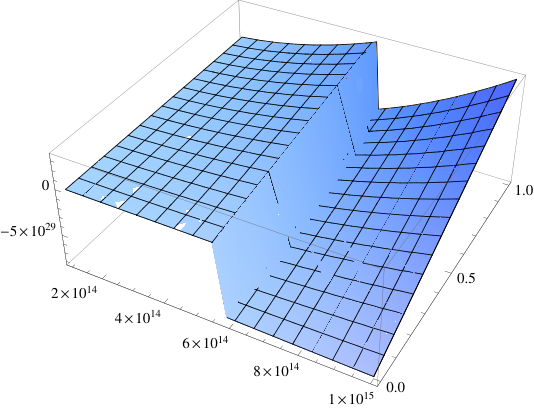
An example of such a transition to a negative gravity region is illustrated in Figure 9, where the surface near the top see-saw scale behaves as in Figure 8.
4.9. Primordial black holes
The possibility of primordial black holes (PBHs) in the early universe was originally suggested by Zeldovich and Novikov in the late 1960s (see [39] for a survey). They originate from the collapse of overdense regions, as well as from other mechanisms such as phase transitions in the early universe, cosmic loops and strings, or inflationary reheating. The consequences on primordial black holes of the running of the gravitational constant in the early universe have been analyzed, for example, in [11]. In models where the gravitational constant in the early universe may be different from the value it has in the modern universe, PBHs, whose existence is conjectured but has not been presently confirmed, are seen as a possible source of information about the changing gravitational constant. In fact, the mass loss rate due to evaporation via Hawking radiation and the Hawking temperature of primordial black holes depends on the value of the Newton constant so that the evolution of such black holes depends on the change in the Newton constant. The evaporation of primordial black holes is often proposed as a mechanism underlying -ray bursts (see for instance [6], [9]). An especially interesting question regarging PBHs is that of gravitational memory, as described in [5]. It is usually assumed that two possible scenarios for the evolution of primordial black holes can happen: one where the evolution follows the changing gravitational constant and one with the possibility of “gravitational memory”, namely where the evolution of the PBH is determined by an effective gravitational constant different from the one of surrounding space. This latter phenomenon can arise if the model has the possibility of having regions, as in the case of the gravity balls discussed in §4.8 above, where the effective gravitational constant has a value different from the one of surrounding space.
We discuss here the effect on primordial black holes of the running of the effective gravitational constant in the noncommutative geometry model. For primordial black holes that formed at a time in the early universe when the gravitational constant was different from the one of the modern universe and whose evolution in time reflects the corresponding evolution of the gravitational constant, the black hole “adjusts its size” to the changing according to the equation
| (4.27) |
where is the mass of the primordial black hole. Correspondingly the temperature varies with the changing gravitational constant as
| (4.28) |
In the case with gravitational memory, one can have a black hole that evolves according to a gravitational constant that is different to the one of the surrounding space. In our setting, given the scenario described in §4.8, this second case occurs with the equation (4.27) replaced by
| (4.29) |
with as in (4.26).
Proposition 4.7.
In the radiation dominated era, for a cosmology with metric tensor of the form (4.13), the evaporation of primordial black holes by Hawking radiation in the NCG model is given by
| (4.30) |
in the case of PBHs without gravitational memory, while PBHs with gravitational memory evaporate according to
| (4.31) |
where
for . Here is the energy scale at which the radiation dominated phase begins, that is, where one starts to have .
Proof.
For a metric of the form (4.13), in the radiation dominated era one has , hence the energy–time change of variables is of the form . Thus, the equation (4.27) can be rewritten in the variable in the form
| (4.32) |
since . We look at the case of a primordial black hole that has a given mass at the initial , and we look at the evolution of between and electroweak scale. The equation (4.32), written in the form
gives (4.30). The case with gravitational memory is obtained similarly by replacing the effective gravitational constant with the one locally modified by the interaction with the Higgs field, . ∎
The expression for the evaporation by Hawking radiation simplifies in the cases where is sufficiently large that the term dominates over . This is the case, for example, when and is chosen accordingly.
Corollary 4.8.
In the case where is sufficiently large that the term is negligible with respect to for all , the evaporation law for a primordial black hole that forms at gives a bound on its mass by .
Proof.
Under the assumption that dominates over , the right hand side of (4.32) can be approximated by the dominant term of which gives
| (4.33) |
Let denote the scale at which the PBH evaporates. Then (4.33) gives
This sets a bound to the mass of a primordial black hole formed at from the condition that
which gives
∎
We can analyze similarly the equation of the Hawking radiation for PBHs during the inflationary epoch when one has for some . We obtain the following result.
Proposition 4.9.
In the inflationary epoch, for a cosmology with metric tensor of the form (4.13), the evaporation of primordial black holes by Hawking radiation in the NCG model is given by
| (4.34) |
in the case of PBHs without gravitational memory, while PBHs with gravitational memory evaporate according to
| (4.35) |
where is the energy scale at which the inflationary behavior begins.
Proof.
The argument is completely analogous to the previous case. Here the energy-time change of variables gives . Thus, in the energy variable the equation (4.27) becomes
for the case without gravitational memory, or the same equation with replaced by in the case with gravitational memory. This gives (4.34) and (4.35). ∎
4.10. Higgs based slow-roll inflation
Recently, a mechanism for inflation within the minimal standard model physics was proposed in [24]. It is based on the presence of a non-minimal coupling of the Higgs field to gravity of the form
as we have in the asymptotic expansion of the spectral action in the noncommutative geometry model, but where the value of is not set equal to the conformal coupling , but is subject to running with the RGE flow. In [24] the running of is governed by the beta function given in [8], which in our notation we can write approximately as
| (4.36) |
where the function of the running parameters of the model is computed explicitly in [8]. In [24] this running is only considered within the minimal standard model, without the right handed neutrinos and Majorana mass terms , but their argument can be adapted to this extension of the standard model, since the general derivation of the running of in [8] applies in greater generality. In this variable scenario, the dimensionless quantity that governs inflation is , where is the reduced Planck mass, which in our notation is . The inflationary period corresponds in [24] to the large values , the end of the inflation to the values and the low energy regime to .
At present we do not know whether a modification of the noncommutative geometry model that allows for a variable , different from the conformal coupling is possible within the costraints of the model, but we show here that, even in the case where is constant in and equal to the conformal , the noncommutative geometry model still allows for a similar inflation mechanism to occur, through the running of the effective gravitational constant.
Proposition 4.10.
A Higgs based slow roll inflation scenario arises in the NCG model with parameter
and with potential
| (4.37) |
Proof.
In the noncommutative geometry model, the coefficient is running with according to
Then the parameter that controls inflation is given by
If one then proceeds as in [24], one finds that In the Einstein metric , for the Higgs potential becomes of the form (4.37). In the range where this approaches the constant function (constant in but not in )
where we used again the ansatz (4.5) for the running of the coefficient , while at low values the potential is well approximated by the usual quartic potential . ∎
The asymptotic value in turn depends on the energy scale and different behaviors are possible upon changing the values of the parameter of the model as the examples in Figure 11 illustrate. One can see the effect of the top see saw-scale on the running.
Notice that a potential of the form as in Figure 10, which is especially suitable for slow roll inflationary models, also arises naturally in the NCG setting from non-perturbative effects in the spectral action, as in [16]. We plan to return in future work to describe how the non-perturbative approach can be applied to cosmological models beyond the very early universe.
4.11. Spectral index and tensor to scalar ratio
In a slow roll inflation model, the first and second derivatives of the potential together with a change of variable in the field that brings the action into a canonical form, determine the first and second slow-roll parameters and , see [34] §3.4 and also the analysis in [24]. We analyze here the form of the slow-roll parameters in the noncommutative geometry model.
We write the potential of (4.37) in the form
| (4.38) |
We will consider derivatives of this potential as a function of the variable .
We also introduce the expression
| (4.39) |
which corresponds to the of equation (4) of [24] that gives the change of variable in the field that runs the inflation that puts the action in a canonical form.
The two slow-roll parameters are then given by the expressions
| (4.40) |
| (4.41) |
which correspond to the equations (6) and (7) of [24]. We then have the following result.
Proposition 4.11.
The first slow roll coefficient is of the form
| (4.42) |
while the second slow-roll coefficient is given by
| (4.43) |
Proof.
Notice that both coefficients depend on the energy scale and on the parameters and through the single parameter
while no dependence through remains and in our model .
The slow-roll coefficients provide expressions for the spectral index and the tensor to scalar ratio , which can be directly compared with cosmological data. Thus, a more detailed analysis of the behavior of these as functions of and of the parameter of the model will give an exclusion curve for the parameter. We will provide a more detailed analysis elsewhere, but for the purpose of the present paper we derive the corresponding expression one has in this model for the spectral index and the tensor to scalar ratio.
Proposition 4.12.
The spectral index is of the form
| (4.44) |
while the tensor to scalar ratio if given by
| (4.45) |
Proof.
Once again, these parameters have a dependence on the choice of the free parameter of the model and a scaling behavior with the energy , which depends on the running of . Since the spectral index and the tensor to scalar ratio are heavily constrained by cosmological data from the WMAP combined with baryon acoustic oscillations and supernovae data, this provides a way to impose realistic constraints on the parameter of the model based on direct confrontation with data of cosmological observations. We will provide a detailed analysis of the constraints imposed on the noncommutative geometry model by the spectral index and tensor to scalar ratio in a separate paper. Since the parameters and are also providing information on the gravitational waves (see [34] §7.7) a more detailed analysis of their behavior and dependence on the parameters of the model will give us a better understanding of the effects on gravitational waves of the presence of noncommutativity and may explain in a different way the amplification phenomena in the propagation of gravitational waves that we observed in §4.4.
4.12. Variable effective cosmological constant
The relation between particle physics and the cosmological constant, through the contribution of the quantum vacua of fields, is well known since the seminal work of Zeldovich [49]. The cosmological constant problem is the question of reconciling a very large value predicted by particle physics with a near zero value that conforms to the observations of cosmology. Among the proposed solutions to this problem are various models, starting with [49], with a varying effective cosmological constant, which would allow for a large cosmological constant in the very early universe, whose effect of negative pressure can overcome the attractive nature of gravity and result in accelerated expansion, and then a decay of the cosmological constant to zero (see also [40] for a more recent treatment of variable cosmological constant models). Often the effective cosmological constant is produced via a non-minimal coupling of gravity to another field, as in [25], similarly to what one does in the case of an effective gravitational constant.
In the present model, one can recover the same mechanism of [25] via the non-minimal coupling to the Higgs field, but additionally one has a running of the effective cosmological constant which already by itself may produce the desired effect of decaying cosmological constant. We illustrate in this section an example of how different choices of the parameter , for a fixed choice of , generate different possible decay behaviors of the cosmological constant. These can then be combined with the effect produced by the non-minimal coupling with the Higgs field, which behaves differently here than in the case originally analyzed by [25]. This still does not resolve the fine tuning problem, of course, because we are trading the fine tuning of the cosmological constant for the tuning of the parameters and of the model, but the fact that these parameters have a geometric meaning in terms of the spectral action functional may suggest geometric constraints.
As we have seen in the proof of Proposition 4.1 above, one can impose the vanishing of the effective cosmological constant at a given energy scale by fixing the parameter equal to the value given in (4.6). This means that, when the effective gravitational constant of the model varies as in the effective gravitational constant surface , depending on the value assigned to the parameter , there is an associated surface that determines the value of the parameter that gives a vanishing effective cosmological constant. This is defined by the equation
| (4.47) |
The solutions to this equation determine the surface
| (4.48) |
To illustrate the different possible behaviors of the system when imposing the vanishing of the effective cosmological constant at different possible energy scales , we look at the examples where one imposes a vanishing condition at one of the two ends of the interval of energies considered, that is, for or for . For simplicity we also give here an explicit example for a fixed assigned value of , which first fixes the underlying . we choose, as above, the particular example where is chosen to satisfy . Under these conditions we impose the vanishing of the effective cosmological constant at either or through the constraint
| (4.49) |
which fixes the value of . Then the behavior at higher energies of the effective cosmological constant is given by the surface
| (4.50) |
as a function of the energy and the parameter .
We find two very different behaviors in these two examples, which have different implications in terms of dark energy. Imposing the vanishing of at produces a very fast growth of at larger energies , while imposing the vanishing at produces a that quicky decreases to a large negative value and then slowly decreases to become small again near , as illustrated in the two examples of Figure 12. A negative cosmological constant adds to the attractive nature of gravity hence it counteracts other possible inflation mechanism that may be present in the model, while a positive cosmological constant counteracts the attractive nature of gravity and can determine expansion. Thus, we see in these two examples that different choices of the free parameter in the model can lead to very different qualitative behaviors of the effective cosmological constant.
The range of different variable cosmological constants can be further expanded by considering other possible values of the parameter in the surface associated to a chosen value of .
Again, as we have seen in the case of the effective gravitational constant, we have here two distinct mechanisms for vacuum-decay: the running as described above, depending on the parameters and and on the renormalization group equations, and a further modification due to the non-minimal coupling with the Higgs field, as in [25].
Namely, if one has an unstable and a stable equilibrium for , one can encounter for the cosmological constant the same type of phenomenon described for the effective gravitational constant by the gravity balls, where the value of is equal to at the unstable equilibrium on some large region, while outside that region it decays to the stable equilibrium for which
This behaves differently in the case of our system from the model of [25]. In fact, here the non-minimal coupling is always the conformal one , while the gravitational constant is itself running, so we obtain the following.
Proposition 4.13.
The non-minimal conformal coupling of the Higgs field to gravity,
changes the running of the effective cosmological constant to
| (4.51) |
This gives
for .
Proof.
Arguing as in [25] we obtain (4.51), which now depends on the running of both and , as well as on the Higgs field . Assuming the latter to be nearly constant with , we obtain
| (4.52) |
where, as in the treatment of the variable effective gravitational constant, we have
using the ansatz (4.5) for , and . ∎
To see how the interaction with the Higgs field can modify the running of the effective cosmological constant, consider again an example that exhibits the same behavior as the second graph of Figure 12. This is obtained, for instance, by choosing and satisfying the vanishing condition . Then the running of given in (4.52) exhibits an overall behavior similar to that of but with a change of sign and a singularity, as shown in Figure 13.
4.13. Early time bounds estimate
In models with variable cosmological (and gravitational) constant, some strong constraints exist from “early time bounds” on the vacuum-energy density that are needed in order to allow nucleosynthesis and structure formation, see [7], [27].
In particular, in our model, this means that we can prefer choices of the parameters and for which the ratio
| (4.53) |
is small at the electroweak end of the energy range we are considering, so that the resulting early time bound will allow the standard theory of big-bang nucleosynthesis to take place according to the constraints of [7], [27].
Notice that, since we have the estimate on (4.53) is independent of further effects of interaction with the Higgs field, and it only depends on the choice of the parameters and of the model.
This type of estimate can be used to select regions of the space of parameters and that are excluded by producing too large a value of (4.53) at . For example, consider the two cases of Figure 12, where we set and we choose so that it gives vanishing at or at . The first case gives , while the second gives a very large negative value of (4.53) at of with a running of (4.53) as in Figure 14.
5. Dark matter
We have concentrated in this paper on early universe models, with an emphasis on various mechanisms for inflation and dark energy that arise within the NCG model, and their mutual interactions. Another main question about cosmological implications of the noncommutative geometry models of particle physics is whether they can accommodate possible models for cold dark matter. This exists the domain of validity of the asymptotic expansion of the spectral action, as such models apply to a more modern universe than what is covered by the perturbative analysis of the spectral action functional. However, one can at least comment qualitatively on possible candidates within the NCG model for dark matter particles. In addition to the minimal Standard Model, one recovers form the computation of the asymptotic formula for the spectral action and from the fermionic part of the action in [17] additional right handed neutrinos with lepton mixing matrix and Majorana mass terms. Thus, since this is at present the only additional particle content beyond the minimal standard model that can be accommodated in the NCG setting, it is natural to try to connect this model to existing dark matter models based on Majorana mass terms for right handed neutrinos.
Those that seem more closely related to what one can get within the NCG model are the ones described by Shaposhnikov–Tkachev [45], Shaposhnikov [44], and Kusenko [33]. In these dark matter models, one has the usual active neutrinos, with very small masses, and an additional number of sterile neutrinos with Majorana masses. In the case of the MSM model of [44], one has three active and three sterile neutrinos. In these models the sterile neutrinos provide candidate dark matter particles. However, for them to give rise to plausible dark matter models, one needs at least one (or more) of the sterile neutrino Majorana masses to be below the electroweak scale. In the detailed discussion given in [33] one sees that, for example, one could have two of the the three Majorana masses that remain very large, well above the electroweak scale, possibly close to unification scale, while a third one lowers below the electroweak scale, so that the very large Majorana masses still account for the see-saw mechanism, while the smaller one provides a candidate dark matter particle.
It is possible to obtain a scenario of this kind within the NCG model, provided that one modifies the boundary conditions of [1] in such a way that, instead of having three see-saw scales within the unification and the electroweak scale, with the smallest one already at at very high energy around GeV, one sets things so that the lowest Majorana mass descends below the electroweak scale. A more detailed analysis of such models will be carried out in forthcoming work where we analyze different choices of boundary conditions for the RGE flow of the model.
6. Conclusions and perspectives
We have shown in this paper how various cosmological models arise naturally from the asymptotic expansion of the spectral action functional in the noncommutative geometry model of particle physics of [17] and the running of the coefficients of this asymptotic expansion via the renormalization group equations of [1].
We have seen in particular the spontaneous emergence of conformal gravity and Hoyle–Narlikar cosmologies at phase transitions caused by the running of the effective gravitational constant. We described effects of this running on the gravitational waves and on primordial black holes. We described mechanisms by which this running, combined with the conformal coupling of gravity to the Higgs field, can generate regions of negative gravity in the early universe. We discussed the running of the effective cosmological constant and slow-roll inflation models induced by the coupling of the Higgs to gravity. We discussed briefly the connection to dark matter models based on right handed neutrinos and Majorana mass terms.
A planned continuation of this investigation will cover the following topics:
- •
Varying boundary conditions for the RGE flow.
- •
Dark matter models based on Majorana sterile neutrinos.
- •
Extensions of the NCG model with dilaton field.
- •
Nonperturbative effects in the spectral action.
- •
Exclusion curve from spectral index and tensor to scalar ratio.
7. Appendix: boundary conditions for the RGE equations
We recall here the boundary conditions for the RGE flow of [1] and we discuss the compatibility with the condition assumed in [17]. A more detailed analysis of the RGE flow of [1] with different boundary conditions and its effect on the gravitational and cosmological terms will be the focus of a followup investigation.
7.1. The default boundary conditions
The boundary conditions for the RGE flow equations we used in this paper are the default boundary conditions assumed in [1]. These are as follows.
For they have
7.2. Constraints from NCG
There are constraints on the boundary conditions at unification in the noncommutative geometry model. Those were described in [17] and we report them here below.
- •
A constraint on the value at unification of the parameter :
- •
A relation between the parameter and the Higgs vacuum:
- •
A constraint on the coefficient at unification, coming from the see-saw mechanism for the right handed neutrinos:
- •
The mass relation at unification:
(7.1) where , , , and are the masses of the leptons and quarks, that is, the eigenvectors of the matrices , , and , respectively, and is the W-boson mass.
Clearly, not all of these constraints are compatible with the default boundary conditions of [1]. So either one relaxes some of these conditions, as we have been doing in the present paper, or one performs a wider search for more appropriate and fine tuned boundary conditions for the RGE flow, analyzing how different choices of boundary values affect the behavior analyzed in this paper. This is presently under investigation.
References
- [1] S. Antusch, J. Kersten, M. Lindner, M. Ratz, M.A. Schmidt Running neutrino mass parameters in see-saw scenarios, JHEP 03 (2005) 024, hep-ph/0501272v3.
- [2] S. Antusch, J. Kersten, M. Lindner, M. Ratz, Neutrino mass matrix running for non-degenerate see-saw scales, Phys.Lett. B538 (2002) 87–95.
- [3] K.S. Babu, C.N. Leung, J. Pantaleone, Renormalization of the neutrino mass operator, Phys. Lett. B, Vol.319 (1993) 191–198.
- [4] J. Barrett, Lorentzian version of the noncommutative geometry of the Standard Model of particle physics. J. Math. Phys. 48 (2007), no. 1, 012303, 7 pp.
- [5] J.D. Barrow, Gravitational memory? Phys. Rev. D Vol.46 (1992) N.8 R3227, 4pp.
- [6] A.A. Belyanin, V.V. Kocharovsky and VI.V. Kocharovsky, Gamma-ray bursts from evaporating primordial black holes, Radiophysics and Quantum Electronics, Vol.41 (1996) N.1, 22–27.
- [7] M. Birkel, S. Sarkar, Nucleosynthesis bounds on a time-varying cosmological ‘constant’, Astroparticle Physics, Vol.6 (1997) 197–203.
- [8] I.L. Buchbinder, D.D. Odintsov, I.L. Shapiro, Effective action in quantum gravity, IOP Publishing, 1992.
- [9] E.V. Bugaev, V.B. Petkov, A.N. Gaponenko, P.A. Klimai, M.V. Andreev, A.B. Chernyaev, I.M. Dzaparova, D.D. Dzhappuev, Zh.Sh. Guliev, N.S. Khaerdinov, N.F. Klimenko, A.U. Kudzhaev, A.V. Sergeev, V.I. Volchenko, G.V. Volchenko, A.F. Yanin, Experimental search of bursts of gamma rays from primordial black holes using different evaporation models, arXiv:0906.3182.
- [10] B. Ćaćić, Moduli spaces of Dirac operators for finite spectral triples, arXiv:0902.2068.
- [11] B.J. Carr, Primordial black holes as a probe of the early universe and a varying gravitational constant, arXiv:astro-ph/0102390v2.
- [12] J.A. Casas, V. Di Clemente, A. Ibarra, M. Quirós, Massive neutrinos and the Higgs mass window, Phys.Rev. D62 (2000) 053005, 4 pp.
- [13] A. Chamseddine, Noncommutative geometry as the key to unlock the secrets of space-time, arXiv:0901.0577.
- [14] A. Chamseddine, A. Connes, The spectral action principle. Comm. Math. Phys. 186 (1997), no. 3, 731–750.
- [15] A. Chamseddine, A. Connes, Why the standard model? Journal of Geometry and Physics, Vol.58 (2008) N.1, 38–47.
- [16] A. Chamseddine, A. Connes, The uncanny precision of the spectral action, arXiv:0812.0165.
- [17] A. Chamseddine, A. Connes, M. Marcolli, Gravity and the standard model with neutrino mixing, Adv. Theor. Math. Phys. 11 (2007), no. 6, 991–1089.
- [18] A. Connes, Geometry from the spectral point of view. Lett. Math. Phys. Vol.34 (1995) N.3, 203–238.
- [19] A. Connes, Gravity coupled with matter and the foundation of non-commutative geometry. Comm. Math. Phys. 182 (1996), no. 1, 155–176.
- [20] A. Connes, Noncommutative geometry and the standard model with neutrino mixing. J. High Energy Phys. 2006, no. 11, 081, 19 pp. (electronic).
- [21] A. Connes, Noncommutative Geometry, Academic Press, 1994.
- [22] A. Connes, M. Marcolli, Noncommutative geometry, quantum fields, and motives. Colloquium Publications, Vol.55, American Mathematical Society, 2008.
- [23] A. Connes, M. Marcolli, A walk in the noncommutative garden, in “An invitation to noncommutative geometry”, pp.1–128, World Scientific, 2008.
- [24] A. De Simone, M.P. Hertzberg, F. Wilczek, Running inflation in the Standard Model, hep-ph/0812.4946v2.
- [25] A.D. Dolgov, An attempt to get rid of the Cosmological constant in “The very early universe” (Eds. G.W. Gibbons, S.W. Hawking, S.T.S. Siklos), Cambridge University Press, 1983, pp. 449
- [26] A. Edery, L. Fabbri, M.B. Paranjape, Spontaneous breaking of conformal invariance in theories of conformally coupled matter and Weyl gravity, hep-th/0603131.
- [27] K. Freese, F.C. Adams, J.A. Frieman, E. Mottola, Cosmology with decaying vacuum energy, Nuclear Physics B, Volume 287 (1987) 797–814.
- [28] R. Gregory, V.A. Rubakov, S.M. Sibiryakov, Gravity and antigravity in a brane world with metastable gravitons, Phys.Lett.B Vol.489 (2000) 203–206.
- [29] U. Guenther, A. Zhuk, V. Bezerra, C. Romero, AdS and stabilized extra dimensions in multidimensional gravitational models with nonlinear scalar curvature terms and , Class.Quant.Grav. 22 (2005) 3135–3167.
- [30] A.H. Guth, Phase transitions in the very early universe, in “The very early universe” (G.W.Gibbons, S.W.Hawking, S.T.C.Siklos, Eds.) pp. 171–204, Cambridge University Press, 1982.
- [31] F. Hoyle, J.V. Narlikar, A new theory of gravitation, Proc. Royal Soc. London. Series A, Mathematical and Physical Sciences, Vol. 282 (1964) No. 1389, 191–207.
- [32] K. Jakobs, M. Schumacher, Prospects for Higgs boson searches at the LHC, in “Perspectives on LHC physics” (G. Kane and A. Pierce, Eds.), World Scientific, 2008, pp. 179–204.
- [33] A. Kusenko, Sterile neutrinos: the dark side of the light fermions, arXiv:0906.2968.
- [34] A.R. Liddle, D.H. Lyth, Cosmological inflation and large-scale structure, Cambrige University Press, 2000.
- [35] A.D. Linde, Gauge theories, time-dependence of the gravitational constant and antigravity in the early universe, Phys. Letters B, Vol.93 (1980) N.4, 394–396.
- [36] D. Lohiya, Non-topological solitons in non-minimally coupled scalar fields: theory and consequences, Astrophysics and Space Science, Vol.232 (1995) 1–22.
- [37] P.D. Mannheim, Alternatives to dark matter and dark energy, Progress in Particle and Nuclear Physics Vol.56 (2006) N.2, 340–445.
- [38] W. Nelson, M. Sakellariadou, Cosmology and the noncommutative geometry approach to the Standard Model, arXiv:0812.1657 [hep-th].
- [39] I.D. Novikov, A.G. Polnarev, A.A. Starobinsky, Ya.B. Zeldovich, Primordial black holes, Astron. Astrophys. 80 (1979) 104–109.
- [40] J.M. Overduin, F.I. Cooperstock, Evolution of the scale factor with a variable comological term, astro-ph/9805260.
- [41] M.D. Pollock, On the proposed existence of an anti-gravity regime in the early universe, Phys. Lett. B, Vol.108 (1982) 386–388.
- [42] M.D. Pollock, Determination of the superstring moduli from the higher-derivative terms, Phys. Lett. B Vol.495 (2000) 401–406.
- [43] M.V. Safonova, D. Lohiya, Gravity balls in induced gravity models – ‘gravitational lens’ effects. Gravitation and Cosmology, (1998) N.1, 1–10.
- [44] M. Shaposhnikov, The MSM, leptonic asymmetries, and properties of singlet fermions, JHEP (2008) 0808:008, 56pp.
- [45] M. Shaposhnikov, I. Tkachev, The MSM, inflation, and dark matter, Phys.Lett. B Vol.639 (2006) 414–417.
- [46] Tevatron New Phenomena, Higgs working group, CDF Collaboration, D0 Collaboration, Combined CDF and Dzero Upper Limits on Standard Model Higgs Boson Production at High Mass (155-200 GeV/c2) with 3 fb-1 of data, arXiv:0808.0534.
- [47] S. Weinberg, Gravitation and Cosmology, John Wiley and sons (1972).
- [48] A. Zee, Broken-symmetry theory of gravity, Phys. Rev. Lett. Vol.42 (1979) 417–421.
- [49] Ya.B. Zeldovich, The cosmological constant and the theory of elementary particles, Sov. Phys. Usp., Vol.11 (1968) 381–393.