Strongly nonlinear dynamics of electrolytes in large ac voltages

In any continuum model, the transport of ions in the electrolyte is governed by a mass conservation law

$$\partial_{t}c_{i}=-\bm{\nabla}\cdot\mathbf{F}_{i},$$

(1)

where $c_{i}$ is the local concentration of the $i$th ionic species, $\mathbf{F}_{i}$ is the flux, and we neglect any bulk reactions in the electrolyte which could produce or consume ions. Quite generally, in a concentrated solution, the flux can be expressed in terms of the gradient of the electrochemical potential $\mu_{i}$ as

$$\mathbf{F}_{i}=-\frac{D_{i}}{kT}\,c_{i}\bm{\nabla}\mu_{i}+\mathbf{u}\,c_{i},$$

(2)

where the first term describes ion transport by diffusion and electromigration with diffusivity $D_{i}$, $k$ is Boltzmann’s constant, $T$ is absolute temperature, and the second term describes advection at the mean fluid velocity $\mathbf{u}$, as determined by momentum conservation. For a dilute solution, the chemical potential $\mu_{i}$ takes the ideal form, with contributions from entropy and mean electrostatic energy,

$$\mu_{i}=kT\log c_{i}+z_{i}e\phi,$$

(3)

where $\phi$ is the electrostatic potential, $z_{i}$ is the ionic valence and $e$ the electron charge. Equation (1) then reduces to the Nernst–Planck equation

$$\mathbf{F}_{i}=-D_{i}\Big(\bm{\nabla}c_{i}+\frac{z_{i}e}{kT}c_{i}\bm{\nabla}\phi\Big)+\mathbf{u}c_{i}.$$

(4)

In the usual mean-field approximation, the electrostatic potential is self-consistently determined by the charge density $\rho$ through Poisson’s equation

$$-\bm{\nabla}\cdot(\varepsilon\bm{\nabla}\phi)=\rho=\sum_{i}z_{i}ec_{i}$$

(5)

where $\varepsilon$ is the electrolyte permittivity, which we take to be constant. This completes the classical PNP equations, which underly most of electrochemical transport theory. As noted above, the characteristic length scale in these equations (the Debye–Hückel screening length) is

$$\lambda_{D}=\sqrt{\frac{\varepsilon kT}{\sum_{i}c_{i}^{*}z_{i}^{2}e^{2}}}.$$

(6)

where $c_{i}^{*}$ is the nominal bulk concentration of the $i$th ionic species.

In the present work we focus on dilute electrolytes for which the nominal bulk salt concentration is small, seemingly within the range of applicability of the PNP equations. Even in a very dilute bulk solution, however, when a large external bias is placed on the electrodes in the system (only a few times $kT/e$), ions accumulate at the surface, and the dilute-solution approximation must break down [53, 57, 58]. Following Kilic et al. [54], we will solve modified (MPNP) equations based on the oldest and simplest approach to steric effects of ion crowding of Bikerman [60], which corresponds to the following model for the chemical potential in a binary $z:z$ electrolyte [54, 74],

$$\mu_{\pm}=kT\log c_{\pm}\pm ze\phi-kT\log(1-c_{+}a^{3}-c_{-}a^{3}),$$

(7)

where $a$ is an effective molecular length scale. (For a history of this model and related concentrated-solution theories, see Ref. [58].) The correction term, which can be interpreted as an activity coefficient $f_{i}=\exp[(\mu_{i}-\mu_{i}^{\mathrm{ideal}})/kT]$, is related to the entropy of the solvent molecules and imposes a maximum ion concentration $c_{\mathrm{max}}=a^{-3}$; it can be derived from the statistical mechanics of of equal-sized ions and solvent molecules on a cubic lattice of spacing $a$ in the continuum limit. In equilibrium, $\mu_{\pm}=$ constant, the ions effectively obey Fermi–Dirac statistics, rather than classical Boltzmann statistics, due to the excluded volume effect [61, 62, 63, 64, 65, 66, 67, 70]. Although more sophisticated models for $\mu_{i}$ exist [54, 74, 58], this approach at least qualitatively captures the effects of volume constraints with only one additional parameter $a$.

For boundary conditions at the (blocking) electrodes, we assume no electrochemical reactions, so the normal ionic fluxes must vanish $\mathbf{n}\cdot\mathbf{F}_{i}=0$. To close the system, we follow many prior authors [80, 10, 81, 1, 45, 16, 11] and allow for a compact (Stern) layer or thin dielectric coating separating the electrode from the electrolyte with a constant “surface capacitance” per unit area $C_{S}$, which leads to a mixed boundary condition

$$C_{S}(V_{\mathrm{ext}}-\phi)+\varepsilon\,\mathbf{n}\cdot\bm{\nabla}\phi=0.$$

(8)

Here $\mathbf{n}$ is a surface normal pointing into the electrolyte, $C_{S}=\varepsilon_{S}/h_{S}$ can be ascribed to a surface coating of thickness $h_{S}$ and dielectric constant $\varepsilon_{S}$, and $V_{\mathrm{ext}}(t)$ is the external potential applied at the electrode.

For the present analysis we focus on a symmetric binary electrolyte with equal diffusivity $D_{+}=D_{-}=D$ and valence $z_{+}=-z_{-}=z$ for the two ionic species. Moreover we restrict our attention to the simplest prototypical microelectrochemical system, consisting of the electrolyte confined between two parallel, planar, blocking electrodes at $x=\pm L$, as sketched in Fig. 1. By symmetry, this rules out any effects of surface conduction [52, 56] or ac electroosmotic flow [9, 10, 11] and allows us to focus on the strongly nonlinear response due to the excessive accumulation of ions in the screening layers at the electrodes. In summary, the system is identical to that studied in Refs. [1] (PNP) and  [54] (MPNP), except that we apply an ac voltage rather than a step dc voltage and study the periodic response after all transients have decayed. We shall see that imposing an external time scale (the ac period) fundamentally alters the dynamics and complicates the analysis.

We cast the problem into dimensionless form using $L$ as the reference length scale and the $RC$ relaxation time $\tau=\lambda_{D}L/D$ as reference time scale [1], so that time and space are represented by the dimensionless variables $t^{\prime}=t/\tau$ and $x^{\prime}=x/L$. The potential and ionic concentrations are rescaled as $\phi^{\prime}=\phi\,ze/kT$ and $c_{\pm}^{\prime}=c_{\pm}/c^{*}$, where $kT/e$ is the thermal voltage scale and $c^{*}$ is the nominal bulk electrolyte concentration.

After dropping the primes from the dimensionless variables, the governing equations take the form

	$\displaystyle-\epsilon^{2}\partial_{x}^{2}\phi$	$\displaystyle=\frac{1}{2}(c_{+}-c_{-}),$		(9)
	$\displaystyle\partial_{t}c_{\pm}$	$\displaystyle=-\epsilon\partial_{x}F_{\pm},$		(10)

where the fluxes $F_{\pm}$ are given by

$$F_{\pm}=-c_{\pm}\partial_{x}\mu_{\pm}.$$

(11)

For a dilute electrolyte the electrochemical potentials reduce to

$$\mu_{\pm}=\log c_{\pm}\pm\phi,$$

(12)

and we arrive at the Nernst–Planck equations in dimensionless form

$$\partial_{t}c_{\pm}=\epsilon\partial_{x}(\partial_{x}c_{\pm}\pm c_{\pm}\partial_{x}\phi).$$

(13)

When steric exclusion is taken into account we get

$$\mu_{\pm}=\log c_{\pm}\pm\phi-\log(1-\nu c),$$

(14)

where the parameter $\nu=2c^{*}a^{3}$ is the nominal volume fraction of the ions in the electrolyte [53].

It is convenient to introduce also the average ion or “salt” concentration and (half) the charge density

$$c=\frac{1}{2}(c_{+}+c_{-})\quad\mbox{and}\quad\rho=\frac{1}{2}(c_{+}-c_{-}),$$

(15)

in terms of which the transport equations can be rewritten as

	$\displaystyle\partial_{t}c$	$\displaystyle=-\epsilon\partial_{x}F,$		(16)
	$\displaystyle\partial_{t}\rho$	$\displaystyle=-\epsilon\partial_{x}J.$		(17)

Here $F=\frac{1}{2}(F_{+}+F_{-})$ and $J=\frac{1}{2}(F_{+}-F_{-})$ are the average salt flux and current density, respectively,

	$\displaystyle F$	$\displaystyle=-\partial_{x}c/(1-\nu c)-\rho\partial_{x}\phi,$		(18)
	$\displaystyle J$	$\displaystyle=-\partial_{x}\rho-c\partial_{x}\phi-\nu\rho\partial_{x}c/(1-\nu c).$		(19)

Since we assume blocking electrodes we have no-flux boundary condition at the electrodes,

$$F_{\pm}=0\quad\mbox{or}\quad F=J=0,$$

(20)

whereas the compact layer b.c. reduces to

$$V_{\mathrm{ext}}-\phi=\mp\epsilon\delta\partial_{x}\phi\quad\mbox{at}\quad x=\pm 1.$$

(21)

Here $V_{\mathrm{ext}}(t)=\mp V\sin(\omega t)$ is the electrode potential and $\delta=C_{D}/C_{S}$ is the ratio of the compact-layer capacitance $C_{S}=\varepsilon_{S}/h_{S}$ to that of the diffuse layer $C_{D}=\varepsilon/\lambda_{D}$ in the low voltage limit.

The PNP model contains three dimensionless parameters: $\epsilon$, $V$, and $\delta$. In aqueous electrolytes, the screening length has submicron scale, $\lambda_{D}\approx 1-100$ nm, so the diffuse-charge boundary layers near the electrodes typically have a very small dimensionless width $\epsilon=\lambda_{D}/L\ll 1$, at least in microsystems where $L\gg 1$ $\mu$m. Although $\epsilon>1$ is possible in nanosystems, we restrict our attention to the typical case $\epsilon\ll 1$, which is the basis for our asymptotic analysis.

Contrary to most prior work, we focus on the nonlinear regime of large applied voltages, $V\gg 1$ (or, with units, $V\gg kT/e\approx 25$ mV), as in Refs. [1, 45, 48, 52, 53, 54]. Since applied voltages larger than a few volts tend to trigger Faradaic reactions in aqueous electrolytes at ac frequencies around the inverse $RC$ time [12, 82], we envision experimentally relevant values of $V\approx 1-200$, although larger voltages can be sustained at higher frequencies or in non-aqueous solvents or liquid salts. Unlike prior work, we allow for large enough voltages that the double-layers lose their quasi-equilibrium structure.

The parameter $\delta=\varepsilon h_{S}/\varepsilon_{S}\lambda_{D}=\lambda_{S}/\lambda_{D}$ (where $\lambda_{S}=h_{S}\varepsilon/\varepsilon_{S}$ is an effective thickness for the compact layer) can be estimated in some cases, but it is usually adjusted to fit experimental data. For example, let us consider different surfaces in contact with a 1 mM aqueous electrolyte with $\lambda_{D}=10$ nm. For a thin dielectic coating, such as a natural TiO₂ oxide layer with $h_{S}=4$ nm and $\varepsilon_{S}=110$ where a constant $C_{S}$ seems reasonable, we get $\delta\approx 0.3$, although much thicker dielectric layers yielding $\delta\approx 10$ can arise in patterned microsystems [17]. In nonlinear electrokinetic phenomena, the inferred value of $\delta$, required to match the standard dilute-solution model to experimental data, can be up to several orders of magnitude larger, although this is more likely due to failures of the model, and not directly related to surface capacitance [58].

With a dielectric electrode coating, the surface capacitance is relatively clear, but in the classical picture of the Stern model [59], it is associated with a hypothetical flat monolayer of water molecules, which limit the approach of hydrated ions at the metal/electrolyte interface. In that case, one would expect $h_{S}\approx 1$ Å, and, since alignment of water dipoles is assumed to reduce the permittivity in the Stern layer to $\varepsilon_{S}\approx 0.1\varepsilon$  [83, 84], we estimate $\delta\approx 0.1$. The Stern picture, however, is complicated (at least) by electronic boundary layers in the metal [85], chemisorption from the solution [86], nanoscale surface roughness [87, 88], and crowding effects absent in the PNP model of the diffuse layer, all of which can be misattributed to the Stern layer, as emphasized by Bazant et al. [58]. Even for a smooth liquid-mercury electrode, the inferred Stern layer capacitance is voltage dependent [83, 86]. Nevertheless, since our goal here is to analyze the nonlinear dynamics of ions in solution, we will simply assume a constant surface capacitance and allow for a wide range of values $\delta=0.01-10$.

In the simple MPNP model there is one more dimensionless parameter, $\nu=2a^{3}c^{*}$, which controls the importance of crowding effects. The nominal concentration $c^{*}$ could range from a very dilute 1 $\mu$M solution with $6\times 10^{20}$ ions/m³ to a concentrated 1 M solution (near physiological salt levels) with $6\times 10^{26}$ ions/m³. A natural choice for the effective molecular lattice spacing $a$ is the diameter of a hydrated ion, around $4-5$ Å for small ions in water, which would yield $\nu\approx 10^{-7}-10^{-1}$. Taking into account the under-estimation of steric effects in a hard-sphere liquid by our lattice-based model [74, 58], the value of $a$ could be increased by roughly a factor of two [69]. Electrostatic correlations also become important when ions are crowded at this scale, comparable to the Bjerrum length, $7$ Å in bulk water. As a crude approximation, therefore, we may consider $\nu$ as large as $0.4$ in a concentrated electrolyte.

Before embarking on our asymptotic analysis, we present some numerical solutions of the PNP model for the problem sketched in Fig. 1, which will be used to test and calibrate various analytical approximations below. As noted above, steric effects in the MPNP model tend to reduce nonlinearities, so the PNP model serves as a more stringent test case.

We use the Comsol finite element package [89] to solve numerically the PNP model in the form of Eqs. (9), (16), and (17) with boundary conditions (20) and (21). It is necessary to use a very fine mesh of $\Delta x_{\mathrm{min}}\approx 10^{-5}$ close to the electrodes in order to resolve the highly compressed (and unphysical) diffuse-layer structure in the PNP model, even at $\epsilon=10^{-3}$. For our 1D problem, this is straightforward to achieve using a nonuniform graded mesh, but in 2D or 3D it would pose a serious problem. In fact, overcoming such limitations is a major motivation for our development of accurate boundary-layer approximations below. The steady-state periodic response is obtained by integrating forward in time, using the default time-dependent solver of Comsol. Since the transient diffusive relaxation in the bulk is slow, it is necessary to integrate for a very long time, up to 100 times the period of the driving voltage or more, before the steady-state periodic solution is reached.

Figure 2 shows the result for $V=30$, $\omega=0.3$, $\delta=0.3$, and $\epsilon=0.001$: Fig. 2(a) shows the potential $\phi(x,t)$, and Fig. 2(b) displays the cation concentration profile $c_{+}(x,t)$. In the bulk region both the cation and anion concentrations are constant and (very close to) unity, and the electrolyte therefore behaves like an ideal resistive medium with unit conductivity. The potential varies linearly throughout the bulk region, driving a constant ohmic current density, and shows a roughly harmonic time variation that is about 45^∘ ahead of the external potential $V_{\mathrm{ext}}=\pm V\sin(\omega t)$ (solid black line at $x=\mp 1$).

In the diffuse screening layer close to the electrodes the ion concentration varies very rapidly from a maximum of $\max\{c_{\pm}\}\approx 3\times 10^{3}$ at the electrode surface down to around unity over a distance of $O(\epsilon)$. The inset in Fig. 2(a) zooms onto the rapid potential variation in the screening layer, and the visible difference between the potential on the electrodes and in the electrolyte corresponds to the compact layer voltage, cf. Eq. (21).

Within a distance of about 0.1 from the electrodes we see a nonuniform pattern in the cation concentration profile that oscillates at twice the driving frequency, $2\omega$. The concentration has a minimum just about the time when the screening layer is fully charged, and a maximum when the screening layer changes polarity (occurs for $t\approx 1.75$ and again at 12.25). The anion concentration shows a fully similar pattern so that effectively this “diffusion layer” is charge neutral.

Figure 3 shows the solution for $V=120$ with otherwise the same parameters as in Fig. 2. The overall picture is essentially the same as before: The bulk ionic concentrations are constant, but due to the massive accumulation of ions around the electrodes (maximal concentration exceeds $4\times 10^{4}$), the bulk concentration is down to 0.86, i.e., 14% below the nominal value.

An interesting feature is seen in Fig. 3(b) for $t\approx 5.24$: Close to the electrode at $x=-1$ there is an extended region where the cation concentration drops to zero, while at the same time the anion concentration is also low but clearly nonzero (see Fig. 14 below for a more detailed view). This transient “space-charge layer” is similar to the steady counterpart described by Rubinstein and Shtilman for the case of dc Faradaic conduction when an electrochemical cell is driven above the diffusion limited current [47, 48]. It is also clear from Fig. 3(a) that there is a significant potential drop across the space-charge layer.

In the limit of thin double layers, $\epsilon=\lambda_{D}/L\ll 1$, the dynamical problem can be analysed by matched asymptotic expansions [1]. The standard procedure begins by seeking regular expansions in the form of power series

$$c=c^{(0)}+\epsilon c^{(1)}+\epsilon^{2}c^{(2)}+\ldots,$$

(22)

substituting into the governing equations, and collecting like powers of $\epsilon$. This procedure is guaranteed to converge in the limit $\epsilon\to 0$ with all other parameters held fixed. However, for any fixed $\epsilon>0$ there could be $\epsilon$-dependent restrictions on the other parameters, in particular the driving voltage $V$, for a truncated expansion to produce accurate results. Following Bazant et al. [1, 52] we denote the regime where such conditions hold as “weakly nonlinear”, as opposed to the “strongly nonlinear” regime where the standard asymptotic expansions breaks down. It is on this “strongly nonlinear” regime that we focus our attention. We aim at deriving the leading-order dominant balance in the joint limit $\epsilon\to 0$ and $V\to\infty$, and since we focus exclusively on the leading-order approximation, we drop the superscript ⁽⁰⁾ on all variables in order to simplify the notation.

For small applied voltages, it is well known that in the limit $\epsilon\to 0$ the diffuse part of the double layer acts as a mathematical boundary layer of $O(1)$ non-zero charge density and $O(\epsilon)$ thickness on the leading-order quasi-electroneutral bulk region at the $O(1)$ length scale of the geometry. This is the mathematical justification for linear circuit models. In the case of blocking electrodes, the characteristic $RC$ time scale for charging of the double layers is $O(1)$ in our dimensionless units.

The application of a large voltage leads to the new effect of salt adsorption by the diffuse layer and related depletion of the bulk concentration, first described by Bazant et al. [1], and in higher dimensions, surface conduction through the diffuse layer becomes important at the same time [52]. For a suddenly applied dc voltage at blocking electrodes, during the initial $RC$ charging phase over $O(1)$ time, a thin quasi-electroneutral diffusion layer extends to $O(\sqrt{\epsilon})$ width. The next phase of relaxation proceeds at the slow $O(\epsilon^{-1})$ time scale for bulk diffusion, as concentration gradients spread across the cell to $O(1)$ distances.

For a large applied ac voltage, this picture is altered by the imposed time scale. In the case of ac forcing close the $RC$ time scale, $\omega^{-1}=O(1)$, the oscillating voltage generally leads to the formation of a thin, nested oscillating diffusion layer confined to steady $O(\sqrt{\epsilon})$ thickness. Since salt adsorption by the inner diffuse layer is positive, regardless of the polarity, the diffusion layer oscillates at twice the driving frequency. It is also accompanied by a gradual bulk salt depletion that propagates across the cell over $O(1)$ times after the ac voltage is turned on, similar to the case of the sudden dc voltage. However, in this work, we ignore such initial transients and focus on the steady ac response after the bulk has relaxed to steady state.

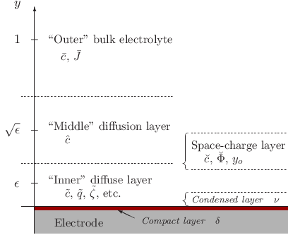
In this way, we are lead to analyze a new, nested boundary-layer structure sketched in Figure 4, consisting of the “outer” bulk region (unit length scale), a “middle” diffusion layer ($\sqrt{\epsilon}$ length scale), and the “inner” diffuse part of the double layer ($\epsilon$ length scale). This picture remains valid until the voltage becomes large enough to fully deplete the middle diffusion layer, leading to the formation of transient space-charge layers extending by $O(\sqrt{\epsilon})$ or more into the cell, twice per ac period. Our goal in the rest of the paper is to develop uniformly valid asymptotic boundary-layer approximations in all of these cases. For clarity, we denote asymptotic approximations for each region by different accents, as indicated Figure  4. For example, the salt concentration $c$ is asymptotic to $\bar{c}$ in the bulk, $\hat{c}$ in the diffusion layer, $\tilde{c}$ in the diffuse charge layer, and $\breve{c}$ in the space-charge layer.

We begin by analyzing the solution in the bulk region. The Poisson equation (9) shows that the charge density vanishes to both zeroth and first order in $\epsilon$ so that at leading order

$$\bar{c}_{+}=\bar{c}_{-}=\bar{c},$$

(23)

denoting bulk variables by a bar accent. The bulk salt concentration displays diffusive dynamics on the time scale $\bar{t}=\epsilon t$ [1], but on the $RC$ time scale the concentration profile is constant in time $\bar{c}=\bar{c}(x)$. Here we focus on the steady state after the bulk transients have relaxed, and by symmetry of our simple model problem, the bulk concentration is then simply constant in space, $\bar{c}=\bar{c}_{o}$. The leading order potential varies linearly in space

$$\bar{\phi}=-\frac{\bar{J}(t)}{\bar{c}_{o}}x,$$

(24)

where $\bar{J}(t)$ is the ohmic current and $\bar{c}_{o}$ acts as the bulk conductivity.

In the weakly nonlinear regime the bulk concentration is at the nominal value, $\bar{c}_{o}=1$, whereas in the strongly nonlinear regime the adsorption of ions in the double layers may be so strong as to induce $\bar{c}_{o}<1$.

The problem has the following symmetries about the origin

$$\left.\begin{array}[]{rcl}\phi(x,t)&=&-\phi(-x,t),\\ \rho(x,t)&=&-\rho(-x,t),\\ c(x,t)&=&\phantom{+}c(-x,t).\end{array}\right\}$$

(25)

In Sections III.3-III.5 below we focus on the nested boundary layers developing at the left electrode, and for convenience we therefore perform a change of variables, $y=1+x$, such that $y=0$ corresponds to the electrode surface and $y\geq 0$ to the interior of the cell.

The singular perturbation in the Poisson equation (9) gives rise to a boundary layer of width $O(\epsilon)$ where the charge density is nonzero to zeroth order in $\epsilon$. Introducing a scaled spatial variable $\tilde{y}=y/\epsilon$ to remove the singular perturbation, we can seek regular asymptotic expansions (denoted by tilde accents) in the “inner” diffuse layer. Substituting into Eqs. (10) and (11) and using $\partial_{\tilde{y}}=\epsilon\partial_{y}$, we find that the double layer is in quasi-equilibrium at leading order with constant electrochemical potential $\tilde{\mu}_{\pm}$ across it. The value of $\tilde{\mu}_{\pm}$ is determined by matching with the solution in the adjacent quasi-electroneutral diffusion layer

$$\tilde{\mu}_{\pm}=\lim_{\hat{y}\to 0}\{\log\hat{c}\pm\hat{\phi}\}.$$

(26)

The quasi-equilibrium arises because the diffuse charge dynamics relaxes on the Debye time scale $\tilde{t}=t/\epsilon$, which is much faster than the $RC$ charging time. The ion distributions are determined from Eq. (14) as

$$\tilde{c}_{\pm}=\frac{\hat{c}_{s}\,e^{\mp\tilde{\psi}}}{1+\nu\hat{c}_{s}(\cosh\tilde{\psi}-1)},$$

(27)

where $\tilde{\psi}=\tilde{\phi}-\hat{\phi}$ is the excess potential in the double layer relative to the diffusion layer, and $\hat{c}_{s}$ is the limiting value of the salt concentration $\hat{c}_{s}=\lim_{y\to 0}\hat{c}$ as seen from the double layer. The excess potential satisfies the MPB equation

$$\partial_{\tilde{y}}^{2}\tilde{\psi}=\frac{\hat{c}_{s}\sinh\tilde{\psi}}{1+\nu\hat{c}_{s}(\cosh\tilde{\psi}-1)},$$

(28)

which can be integrated once to get the field [68, 53]

$$\partial_{\tilde{y}}\tilde{\psi}=-\mathrm{sign}(\tilde{\psi})\sqrt{2\log[1+2\nu\hat{c}_{s}\sinh^{2}(\tilde{\psi}/2)]/\nu}.$$

(29)

Note that the ion concentrations in Eq. (27) are bounded above by steric exclusion, $\tilde{c}_{\pm}\leq 2/\nu$, while at much lower concentrations they reduce to the usual results from dilute theory: In this limit ($\nu\to 0$) the ion profiles are given by the Boltzmann equilibrium distribution,

$$\tilde{c}_{\pm}=\hat{c}_{s}e^{\mp\tilde{\psi}},$$

(30)

and we obtain the standard PB equation

$$\partial_{\tilde{y}}^{2}\tilde{\psi}=\hat{c}_{s}\sinh\tilde{\psi},$$

(31)

yielding the familiar Gouy–Chapman (GC) solution

$$\tilde{\psi}=4\tanh^{-1}\!\Big[\tanh\!\big(\tilde{\zeta}/4\big)e^{-\sqrt{\hat{c}_{s}}\,\tilde{y}}\Big].$$

(32)

Here the integration constant $\tilde{\zeta}=\tilde{\psi}(0)$ is simply the leading order zeta potential, and $1/\sqrt{\hat{c}_{s}}$ is the local effective Debye length.

The redistribution of ions across the diffuse layer is instantaneous on the $RC$ time scale, but the total amount of ions absorbed can change only by flux into the layer from the adjacent diffusion layer. Following Bazant et al. [1, 52, 56, 53, 54] we quantify this by considering the excess amount of each ionic species accumulated in the double layer, $w_{\pm}=\epsilon\tilde{w}_{\pm}$, where

$$\tilde{w}_{\pm}=\frac{1}{\epsilon}\int_{\textrm{d.l.}}\big(\tilde{c}_{\pm}-\hat{c}_{\pm}\big)\,\mathrm{d}y=\int_{0}^{\infty}(\tilde{c}_{\pm}-\hat{c}_{\pm})\,\mathrm{d}\tilde{y}.$$

(33)

The time evolution of $\tilde{w}_{\pm}$ is then determined by

	$\displaystyle\partial_{t}\tilde{w}_{\pm}$	$\displaystyle=\int_{0}^{\infty}\partial_{t}\big(\tilde{c}_{\pm}-\hat{c}_{\pm}\big)\,\mathrm{d}\tilde{y}=-\lim_{\tilde{y}\to\infty}\tilde{F}_{\pm}$		(34)
		$\displaystyle=-\lim_{\hat{y}\to 0}\hat{F}_{\pm},$		(35)

where the last equality is obtained by flux matching between the double layer and diffusion layer. We also define the diffuse charge and excess salt concentration by

$$\tilde{q}=\frac{1}{2}(\tilde{w}_{+}-\tilde{w}_{-})\quad\mbox{and}\quad\tilde{w}=\frac{1}{2}(\tilde{w}_{+}+\tilde{w}_{-}).$$

(36)

Since the diffusion layer is quasi-electroneutral at leading order, the double-layer charging process is coupled directly to the bulk electric current

$$\partial_{t}\tilde{q}=-\bar{J}(t).$$

(37)

Variations in the excess salt $\tilde{w}$ are coupled to the dynamics in the diffusion layer

$$\partial_{t}\tilde{w}=-\lim_{\hat{y}\to 0}\hat{F}\equiv-\tilde{F}_{o},$$

(38)

where the flux injection $\tilde{F}_{o}(t)$ at the inner “edge” of the diffusion layer should be understood as the driving force behind the oscillations in the salt concentration in the diffusion layer. These relations exemplify the general mathematical theory of surface conservation laws, in which the total excess concentrations in a diffuse interface are coupled to normal (and surface) fluxes in a concentrated solution [56].

The diffuse screening layers at the electrodes periodically absorb and expel an excess amount of ions from the surrounding electrolyte. However, the bulk transport of neutral salt is essentially a diffusion process on the time scale $\bar{t}=\epsilon t$, which is much slower than the ac driving that we consider here, and hence the leading order dynamics are confined to a diffusion layer of $O(\sqrt{\epsilon})$ width around the electrode [1, 52]. We therefore introduce a scaled spatial variable $\hat{y}=y/\sqrt{\epsilon}$ and seek regular asymptotic expansions (denoted by hat accents) in this “middle” diffusion layer. Substituting into the Poisson equation (9) we find that, like in the bulk, the charge density vanishes to zeroth order in $\epsilon$, so that the leading order ion concentrations are equal

$$\hat{c}_{+}=\hat{c}_{-}=\hat{c}.$$

(39)

Equation (16) then reduces to a simple diffusion problem

$$\partial_{t}\hat{c}=\partial_{\hat{y}}^{2}\hat{c},$$

(40)

to be solved on the interval $\hat{y}\in[0,\infty)$. Matching to the bulk solution requires $\lim_{\hat{y}\to\infty}\hat{c}\sim\lim_{y\to 0}\bar{c}=\bar{c}_{o}$, whereas the boundary condition at the inner edge of the diffusion layer is determined by matching with the salt flux out of the double layer, cf. Eq. (38)

$$-\frac{1}{\sqrt{\epsilon}}\lim_{\hat{y}\to 0}\partial_{\hat{y}}\hat{c}=\lim_{\hat{y}\to 0}\hat{F}=\tilde{F}_{o}.$$

(41)

The solution to the 1D diffusion problem can be expressed in terms of a convolution integral [1]

$$\hat{c}=\bar{c}_{o}+\sqrt{\epsilon}\int_{-\infty}^{t}G(\hat{y},t-t^{\prime})\tilde{F}_{o}(t^{\prime})\,\mathrm{d}t^{\prime},$$

(42)

where

$$G(\hat{y},t)=\frac{1}{\sqrt{\pi t}}e^{-\hat{y}^{2}/4t}$$

(43)

is the Green’s function for the diffusion equation with a sudden unit flux at $t=0^{+}$ injected at the boundary,

$$G(\hat{y},0)=0,\quad-\partial_{\hat{y}}G(0^{+},t)=\delta^{+}(t).$$

(44)

for a semi-infinite domain. Technically, Eq. (43) is the first term in an expansion for the Green function in a finite bulk domain (Eq. 24 of Ref. [1]), which would be needed to describe the initial transient when the ac voltage is first turned on. Here, we focus on the steady-state response, after initial diffusion layers have relaxed across the cell, thereby lowering the uniform bulk concentration $\bar{c}$ (see below), and the oscillating diffusion layers have only $O(\sqrt{\epsilon})$ width, consistent with the semi-infinite approximation (43).

To describe this situation, since the flux injection is periodic we may rewrite Eq. (42) as

$$\hat{c}=\bar{c}_{o}+\sqrt{\epsilon}\int_{0}^{T}G_{\omega}(\hat{y},t-t^{\prime})\tilde{F}_{o}(t^{\prime})\,\mathrm{d}t^{\prime},$$

(45)

where $T=2\pi/\omega$ is the driving period and

$$G_{\omega}(\hat{y},t)=\frac{1}{T}\bigg[-\hat{y}+\sum_{n=1}^{\infty}\frac{1}{\sqrt{in\omega}}\,e^{in\omega t-\sqrt{in\omega}\hat{y}}+\mathrm{c.c.}\bigg]$$

(46)

is the Green’s function for a periodic influx of salt,

$$\langle G_{\omega}(0,t)\rangle=0,\ -\partial_{\hat{y}}G_{\omega}(0^{+},t)=\sum_{n=-\infty}^{\infty}\delta^{+}(t-nT).$$

(47)

Equations Eqs. (42) or (45) clearly show that in the weakly nonlinear regime, where $\tilde{F}_{o}$ is $O(1)$, the concentration in the diffusion layer $\hat{c}$ is equal to the bulk $\bar{c}$ at leading order; the flux injection only gives rise to an $O(\sqrt{\epsilon})$ perturbation. The strongly nonlinear regime is essentially defined as the regime of driving voltages high enough that $\tilde{w}$ and $\tilde{F}_{o}$ grows to $O(1/\sqrt{\epsilon})$ and the variations in $\hat{c}$ reach $O(1)$.

Since the diffusion layer is charge neutral at leading order, the current is constant across it and equal to the bulk current $\bar{J}(t)$. However, the conductivity differs from its bulk value, which gives rise to transient concentration polarization. There is an excess electrostatic potential variation $\hat{\psi}=\hat{\phi}-\bar{\phi}$, and an excess field given by

$$-\frac{1}{\sqrt{\epsilon}}\partial_{\hat{y}}\hat{\psi}=\bar{J}\bigg(\frac{1}{\hat{c}}-\frac{1}{\bar{c}}\bigg).$$

(48)

In the weakly nonlinear regime when $(1/\hat{c}-1/\bar{c})$ is $O(\sqrt{\epsilon})$ it is clear that $\hat{\psi}$ is only an $O(\epsilon)$ perturbation; in the strongly nonlinear regime $\hat{\psi}$ grows to $O(\sqrt{\epsilon}\bar{J})$ perturbation which is, however, still negligible compared to the bulk $\bar{\phi}=-\bar{J}x/\bar{c}_{o}$.

Finally, the leading order charge density in the diffusion layer can be evaluated by substituting Eq. (48) into the Poisson equation to get

$$\hat{\rho}=-\epsilon\partial_{\hat{y}}^{2}\hat{\psi}=-\epsilon^{3/2}\frac{\bar{J}\partial_{\hat{y}}\hat{c}}{\hat{c}^{2}}.$$

(49)

The quasi-electroneutral solution in the diffusion layer remains valid for $|\hat{\rho}|\ll\hat{c}$; we return to this aspect in Sec. VI.

In order to close the coupled problem for the dynamical variables $\bar{J}(t)$, $\tilde{q}(t)$, $\tilde{\zeta}(t)$, $\tilde{w}(t)$, and $\hat{c}_{s}(t)$ we need a few more relations between them. The first is obtained by writing the overall potential drop over the boundary layers, from the electrode to the bulk electrolyte at $x=-1$, as the sum of the contributions from the compact and diffuse layers, to get

$$V_{\mathrm{ext}}-\bar{\phi}(-1,t)=V_{\mathrm{ext}}-\bar{J}/\bar{c}_{o}=-\tilde{q}\,\delta+\tilde{\zeta}.$$

(50)

Since we focus on the leading order approximation, we neglect here the small potential drop over the diffusion layer. Next, the diffuse-layer voltage $\tilde{\zeta}$ can be related to the diffuse charge through Eq. (29) for the field at the electrode surface, yielding

$$\tilde{q}=-\mathrm{sign}(\tilde{\zeta})\sqrt{2\log[1+2\nu\hat{c}_{s}\sinh^{2}(\tilde{\zeta}/2)]/\nu},$$

(51)

and in the dilute limit this reduces to Chapman’s formula

$$\tilde{q}=-2\sqrt{\hat{c}_{s}}\sinh(\tilde{\zeta}/2).$$

(52)

The charge-voltage relation can be inverted to get

$$\tilde{\zeta}=-\mathrm{sign}(\tilde{q})\,2\sinh^{-1}\sqrt{\frac{e^{\nu\tilde{q}^{2}/2}-1}{2\nu\hat{c}_{s}}}.$$

(53)

The excess salt concentration can be expressed in integral form [54]

$$\tilde{w}=\int_{0}^{\tilde{\zeta}}\frac{\tilde{c}}{\partial_{\tilde{y}}\tilde{\psi}}\,\mathrm{d}\tilde{\psi},$$

(54)

and using PB theory in the dilute limit the integral can be evaluated to get [1]

$$\tilde{w}=4\sqrt{\hat{c}_{s}}\sinh^{2}(\tilde{\zeta}/4),$$

(55)

or, eliminating $\tilde{\zeta}$ we obtain

$$\tilde{w}=\sqrt{\tilde{q}^{2}+4\hat{c}_{s}}-\sqrt{4\hat{c}_{s}}.$$

(56)

For the MPB model, Eq. (54) is difficult to handle analytically, but numerical integration shows that Eq. (56) approximates the integral well, with relative error of $O(\nu)$.

The bulk salt concentration $\bar{c}_{o}$ is determined by imposing the global conservation of salt in the cell

$$\int_{-1}^{1}c(x,t)\,\mathrm{d}x=2.$$

(57)

As noted in Ref. [45], integral constraints on the total number of inactive ions are generally required for steady-state problems to replace information about the initial condition (e.g. when the voltage is first turned on) that is preserved during time evolution with no-flux boundary conditions.

There is a periodic exchange of salt between the inner diffuse and middle diffusion layers, but Eq. (45) shows that $\langle\hat{c}\rangle=\bar{c}$, i.e., the diffusion layer does not contain any excess salt on time average. As a result, the uniform bulk concentration in the (time-periodic) steady state, $\bar{c}_{o}$ , is reduced only by the time-averaged salt adsorption of the diffuse layers,

$$\bar{c}_{o}=1-\epsilon\langle\tilde{w}\rangle.$$

(58)

which also describes the (static) steady state after a sudden dc voltage is imposed [1]. This, together with Eqs. (37), (38), (45), (50), (53), and (56) constitute a set of “ordinary” integro-differential-algebraic equations in time for the dynamical variables $\bar{J}(t)$, $\tilde{q}(t)$, $\tilde{F}_{o}(t)$, $\tilde{w}(t)$, $\hat{c}_{s}(t)$, and $\tilde{\zeta}(t)$.

Our focus in the present work is on the steady-state periodic response, and we explicitly made use of this in deriving our dynamical model by replacing the transient Eq. (43) with Eq. (46). The problem could be solved numerically by a relaxation method, representing each dynamical variable by a truncated Fourier series, as done in Ref. [75]. Here, however, our approach is to integrate the dynamical equations by a timestepping algorithm; the integration is continued until a periodic state is reached, typically within 10-20 periods of the driving voltage. The timestepping approach is well suited for integrating also the non-equilibrium model developed in Sec. VI, and is much more efficient on computer memory for solving problems with 2D or 3D electrode geometry. Further details are given in our supplementary material [90].

The only nonlinearity in the weakly nonlinear model arises from the diffuse-layer charge-voltage relation, Eq. (51). In Fig. 5 we plot the accumulated charge $\tilde{q}$ as a function of the overall potential drop $\tilde{\Psi}=\tilde{\zeta}-\tilde{q}\,\delta$ across the double layer for different values of the capacitance ratio $\delta$ and nominal ion volume fraction $\nu$.

In the Debye–Hückel limit, $\tilde{\zeta}\ll 1$, Eq. (51) can be linearized to get simply $\tilde{q}=-\tilde{\zeta}=-\tilde{\Psi}/(1+\delta)$. At larger voltage the classical PB theory predicts a dramatic increase in the diffuse-layer capacitance, and $\tilde{q}$ grows exponentially with $\tilde{\zeta}$. In Fig. 5 this behaviour shows directly on the curve $\delta=\nu=0$ (Gouy–Chapman (GC) model) that bends up sharply for $\tilde{\Psi}\gtrsim 10$; at $\tilde{\Psi}=20$ the concentration in the diffuse layer, cf. Eq. (30), exceeds $10^{8}$ times the bulk concentration, which is absurdly high for aqueous electrolytes.

This well-known unphysical artifact of PB theory is alleviated (but not eliminated) in the Gouy–Chapman–Stern (GCS) model by assuming a finite compact layer capacitance, corresponding to a positive value of $\delta$. Then at large voltage the major part is carried by the compact layer, $\tilde{\Psi}\approx-\tilde{q}\,\delta$, while the diffuse-layer voltage remains small, $|\tilde{\zeta}|\approx 2\log|\tilde{q}|\approx 2\log|\tilde{\Psi}/\delta|$. This regularizes the problem at moderate voltages, but the success may be misleading: It is unlikely that an ångström-thick molecular Stern layer could withstand several volts without dielectric breakdown. Moreover, the GCS model does not impose a maximum charge density and at sufficiently large voltages still reaches unphysical ion concentrations.

A more realistic approach could account for crowding effects at large voltages using MPB theory [53, 58], e.g. leading to Bikerman’s model described above [60]. This is equivalent to PB theory at concentrations well below the limit of steric exclusion, $\tilde{c}_{\pm}\ll 2/\nu$, as seen clearly in Fig. 5. However, once steric effects saturate the charge density, the diffuse-layer capacitance quickly drops due to the condensed phase of ions forming at the electrode [59, 68, 53, 58]. This occurs for $\tilde{q}^{2}\gtrsim 2/\nu$, and at still larger voltage the overall potential drop is primarily on the condensed layer, with Eq. (51) reducing to

$$|\tilde{q}|\approx\sqrt{\frac{2|\tilde{\zeta}|}{\nu}}\approx\sqrt{\frac{2|\tilde{\Psi}|}{\nu}}\ \mbox{ for }\ |\tilde{\Psi}|\gg\frac{2}{\nu}$$

(59)

Comparing the GCS model for a Stern monolayer with $\delta=0.03$ to Bikerman’s model, the latter predicts (much) lower charging already for $\tilde{\Psi}\gtrsim 30$ (or 750 mV) at $\nu=10^{-4}$. Even for our example of an oxide layer on the electrodes with $\delta=0.3$, crowding effects in the liquid could significantly affect the charge-voltage response for $\tilde{\Psi}\gtrsim 100$ (or 2.5 V), which is still within the range of many experiments.

This asymptotic square-root dependence of the charge-voltage relation (59) is a generic consequence of volume constraints [58], not only in Bikerman’s lattice-gas model, but also hard-sphere liquid models, since it corresponds to a diffuse layer of uniform charge density. Once the condensed layer forms, its voltage $\tilde{\zeta}\approx\nu\tilde{q}^{2}/2$ can easily exceed that of the outer (PB) part of the diffuse layer $\tilde{\zeta}\approx 2\log(\tilde{q})$, even while the latter remains thicker. In this regime of the model, the thickness of the condensed layer is $\tilde{\ell}=\ell/\epsilon\approx\nu\tilde{q}$, which does not become larger than the diffuse-layer thickness until $\tilde{q}>1/\nu$.

The leading order dynamic response in the weakly nonlinear regime is governed by

	$\displaystyle\partial_{t}\tilde{q}$	$\displaystyle=-\bar{J},$		(60)
	$\displaystyle V_{\mathrm{ext}}-\bar{J}$	$\displaystyle=\tilde{\zeta}-\tilde{q}\,\delta,$		(61)
	$\displaystyle\tilde{\zeta}$	$\displaystyle=2\sinh^{-1}\sqrt{\frac{e^{\nu\tilde{q}^{2}/2}-1}{2\nu}}$		(62)
	$\displaystyle\hat{c}$	$\displaystyle=\bar{c}=1.$		(63)

This may be rewritten as a single ordinary differential equation for the double-layer voltage $\tilde{\Psi}$ [1]

$$C\,\partial_{t}\tilde{\Psi}=\bar{J}=V_{\mathrm{ext}}-\tilde{\Psi},$$

(64)

where $C(\tilde{\Psi})=-\mathrm{d}\tilde{q}/\mathrm{d}\tilde{\Psi}$ is the total differential capacitance of the double layer, and $V_{\mathrm{ext}}(t)=V\sin(\omega t)$ is the external driving voltage.

We focus on the periodic response obtained by starting from an initially uncharged state and integrating forward in time until all transients have died out. Figure 6 shows the results for different values of the model parameters:

Fig. 6(a) shows the result for $V=1$, $\omega=1$, $\delta=0.3$, and $\nu=0$. At this low voltage the charge-voltage relation is still essentially linear, so the system behaves like a linear $RC$ circuit with time constant $(1+\delta)^{-1}$. The double-layer voltage $\tilde{\Psi}$ is dominated by the diffuse layer with the compact layer contributing only a small fraction $\delta$.

Figure 6(b) shows the solution at larger voltage $V=30$ with $\omega=0.5$, $\delta=0.3$, and $\nu=0$. At this voltage the relation between $\tilde{\zeta}$ and $\tilde{q}$ is clearly nonlinear, $\tilde{\zeta}$ stalls for $|\tilde{q}|\gtrsim 10$, and the double-layer voltage becomes dominated by the compact layer. When the double layer changes polarity this in turns makes the change of sign of $\tilde{\zeta}$ look like a “sharp” transition which gives rise to a jump in the bulk current. Those features are even more pronounced in Fig. 6(c), showing the corresponding solution for $\delta=0$, i.e., without any compact layer on the electrodes. The double-layer voltage remains low so the bulk current is almost in phase with the driving voltage.

As discussed in the previous section, the very large capacitance of the diffuse layer predicted by PB theory is not realistic. For the solution in Fig. 6(c) the maximal ion concentration in the diffuse layer almost reaches $10^{4}$ times the bulk concentration, which could easily trigger steric effects, even for a nominally dilute electrolyte. Figure 6(d) shows the result when such are taken into account with a bulk volume fraction $\nu=0.01$. The result is markedly different: When steric effects set in, the diffuse-layer capacitance drops and $\tilde{\zeta}$ grows rapidly with $\tilde{q}$. At lower charging, though, the system is still governed by dilute theory, so we still see a rapid shift in $\tilde{\zeta}$ with an associated jump in $\bar{J}$ when the double layer changes polarity.

A useful concept for analyzing the cell response is an equivalent circuit diagram like that shown in Fig. 7(a). The transport through the bulk electrolyte is represented by an ohmic resistor $2R=2$, and the charge accumulation in the double layer by a series coupling of two capacitors $C_{S}$ and $C_{D}$

$$\frac{1}{C}=\frac{1}{C_{S}}+\frac{1}{C_{D}}.$$

(65)

Here $C_{S}=1/\delta$ is the capacitance of the compact (Stern) layer, and $C_{D}=-d\tilde{q}/d\tilde{\zeta}$ is the differential capacitance of the diffuse (Debye) layer, given by [68, 53, 70, 58]

$$C_{D}=\frac{|\sinh\tilde{\zeta}|}{\big[1+2\nu\sinh^{2}(\tilde{\zeta}/2)\big]\sqrt{2\log\big[1+2\nu\sinh^{2}(\tilde{\zeta}/2)\big]/\nu}}.$$

(66)

In the Debye–Hückel limit this reduces to $C_{D}=1$ and $C=1/(1+\delta)$. At higher voltage, PB theory predicts a dramatic increase of $C_{D}=\cosh(\tilde{\zeta}/2)$, to the extent that $C\approx 1/\delta$. According to MPB theory, the diffuse-layer capacitance becomes a non-monotonic function of $\tilde{\zeta}$, where the initial increase is followed by a decrease as $C_{D}\approx 1/\nu\tilde{q}\approx 1/\sqrt{2\nu\tilde{\zeta}}$ once steric exclusion sets in.

The equivalent circuit representation is useful for understanding and interpreting the system response. However, from an experimental point of view the overall cell impedance is a key property that can easily be measured with high accuracy, e.g., using a lock-in amplifier. We define the (half) cell impedance $Z$ as the ratio between the first Fourier components of the applied voltage and the resulting current

$$Z=\frac{\int_{0}^{T}V_{\mathrm{ext}}(t)\,e^{-i\omega t}\,\mathrm{d}t}{\int_{0}^{T}\bar{J}(t)\,e^{-i\omega t}\,\mathrm{d}t}.$$

(67)

Since the system is nonlinear, the impedance so defined is a function of both driving frequency and voltage. Figure 7(b) shows a Bode plot of the cell impedance $Z$ for different values of $V$ at $\delta=0.3$ and $\nu=0$. The curve shape is characteristic of an $RC$ series coupling. At high frequency the ohmic resistance of the bulk electrolyte dominates and $|Z|$ levels off at unity, while at low frequency the double-layer capacitance dominates and $|Z|\propto\omega^{-1}$. At the same time the phase angle $\angle Z$ drops from zero at high frequency to $-90^{\circ}$ at low frequency. We define the characteristic frequency $\omega_{o}$ for a given driving voltage as that frequency where the phase angle passes through $-45^{\circ}$, i.e.,

$$\angle Z(\omega_{o})=-45^{\circ}.$$

(68)

At this frequency the resistive and capacitive components contribute equally much to the overall cell impedance. Figure 7(b) clearly shows that as the voltage is increased, the double-layer capacitance grows, and the characteristic frequency shifts down.

The voltage dependence of $\omega_{o}$ is shown in more detail in Fig. 8, where $\omega_{o}$ is plotted versus $V$ for different values of $\delta$ and $\nu$. The GCS model simply predicts $\omega_{o}$ should drop from $\omega_{o}=1+\delta$ at low voltage to $\omega_{o}\approx\delta$ at higher voltage. The same trend is seen for the Bikerman model, up to the point where steric exclusion sets in; beyond this the double-layer capacitance decreases and $\omega_{o}$ increases, scaling as $\omega_{o}=O(\sqrt{\nu V})$ at large voltage. These qualitative features predicted by our analysis may be interesting to compare to experimental impedance measurements at large ac voltages, below the threshold for Faradaic reactions or specific adsorption of ions, to seek evidence of steric effects in the liquid phase.

In response to the ac driving, the diffuse layer periodically absorbs and expels an excess amount of ions. At low voltage the charging comes about from both uptake of counterions and expulsion of coions, so the net salt adsorption is low, $\tilde{w}\approx\tilde{q}^{2}/4$, cf. Eq. (56) for $\tilde{q}\ll 1$. At higher voltage there are essentially no more coions to expel, so the charging process is dominated by uptake of counterions and $\tilde{w}\approx|\tilde{q}|$.

The excess amount of (counter) ions is taken up from both the adjacent diffusion layer and from that at the opposite electrode. In order to estimate when this effect starts to significantly perturb the concentration in the diffusion layer, it is necessary to know the time-average salt uptake $\langle\tilde{w}\rangle$. This is shown in Fig. 9 as a function of driving voltage and frequency for the Bikerman model with $\delta=0$ and $\nu=0.01$. At low frequency, $\omega\ll\omega_{o}$, the double layer is almost fully charged, so that $\tilde{\Psi}\approx V_{\mathrm{ext}}$. At low voltage, $V\lesssim 1$, the figure shows that $\langle\tilde{w}\rangle\approx V^{2}/8$, while at high voltage, $V\gtrsim 30$, the steric effects dominate and $\langle\tilde{w}\rangle\approx\sqrt{V/\nu}$. For comparison, the GCS model predicts $\langle\tilde{w}\rangle\approx 2V/\pi\delta$ in this limit, and the GC model $\langle\tilde{w}\rangle\approx\exp(V/2)$. At high frequency, $\omega\gg\omega_{o}$, the bulk resistance dominates the cell impedance, so $\bar{J}\approx V_{\mathrm{ext}}$ and $\tilde{q}=O(\bar{J}/\omega)$, from which the scaling is $\langle\tilde{w}\rangle\approx V^{2}/8\omega^{2}\lesssim 1$ or $\langle\tilde{w}\rangle\approx 2V/\pi\omega\gtrsim 10$, depending on the level of charging.

The weakly nonlinear regime in a blocking electrolytic cell generally breaks down at large voltages, when the neutral salt adsorption is by the diffuse layers is strong enough to significantly deplete the quasi-neutral bulk solution in the diffusion layers [1, 52, 53, 54]. This phenomenon, however, relies on the availability of available space in the liquid (free of ions) for the total density of ions to become much more concentrated in one region (the double layers) at the expense of another region (the bulk diffusion layers), which is controlled in our MPNP model by the parameter $\nu=2a^{3}c^{*}=2c^{*}/c_{\mathrm{max}}$. In liquid electrolytes, $\nu$ represents the bulk volume fraction of (all) solvated ions, which is typically much less than one, and even in saturated solutions of highly soluble ions would rarely exceed 0.1. As such, strongly nonlinear effects must generally be considered (below) in electrolytes at large applied voltages, especially in small systems.

The situation is different in ionic liquids or molten salts, which may be described by the limit $\nu\to 1$ in our MPNP model. This corresponds to the mean-field theory proposed by Kornyshev [70] where a value $\nu<1$ could model a somewhat lower volume fraction of the quasi-neutral bulk liquid phase, compared to the charged double layers, where strong normal electric fields may compress the counterions against a charged surface (as described above). In a molten salt, this density variation may be comparable to the expansion upon melting of an ionic crystal, which can be as large as 20%, so we might expect $\nu$ to be as small as 0.8, which is still much larger than for a typical electrolyte. This simple approach has had some success in describing experiments and simulations of simple ionic liquids [71, 72], in what we would call a weakly nonlinear approximation, where the voltage-dependent quasi-equilibrium double-layer capacitance is coupled to a constant bulk resistor.

An important prediction of our analysis is that this picture always remains valid up to large applied voltages for sufficiently large $\nu$, so that ionic liquids can generally be described by the simple, weakly nonlinear approximation. For a highly concentrated electrolyte (still with $\nu\ll 1$), we can use the estimate of Kilic et al. [54] for the critical voltage $V_{c}$ (defined by $\epsilon\langle\tilde{w}\rangle=1$) to significantly deplete the steady-state bulk salt concentration,

$$V_{c}\approx\frac{\nu}{2\epsilon^{2}}=\frac{2(ze)^{2}L^{2}a^{3}c^{*2}}{\varepsilon kT}\propto\left(\frac{c^{*}}{c_{\mathrm{max}}}\right)^{2}$$

(69)

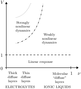
which grows with concentration like $\nu^{2}$ (for fixed ion size). The basic picture is sketched in Fig. 10, where this transition is represented by the dotted line. Before this transition is reached, the weakly nonlinear approximation breaks down due to significant concentration variations, which are not large enough to deplete the bulk and remain confined to the diffusion layers. We estimate and discusse these transitions below in terms of voltage, but here we note that they also rise steeply with concentration in the limit of ionic liquids, $\nu\to 1$. In a molten salt $\nu\approx 1$, the strongly nonlinear regime disappears, and the nonlinear RC circuit approximation holds for all voltages.

The weakly nonlinear dynamics of ionic liquids in the MPNP model are not very different from those of concentrated electrolytes at large enough voltages to trigger steric effects in the double layer. In Figs. 5 and 8 we have also included curves for $\nu=0.1$ and $\nu=1.0$.

Figure 11 shows the strongly nonlinear dynamic response at at $V=30$, $\omega=0.3$, $\delta=0.3$, $\nu=0$, and $\epsilon=0.001$. First off we note that the qualitative difference against the weakly nonlinear solution from Fig. 6(b) is fairly small, even though the surface concentration $\hat{c}_{s}$ shows a significant variation. Quantitatively the largest difference is on the zeta potential, reaching 12% relative difference between the weakly and strongly nonlinear models. Perhaps this should not be too surprising: The surface concentration affects the double-layer charging dynamics only through the diffuse-layer charge-voltage relation, Eq. (51), and only in a square-root dependence. Moreover, at this voltage the diffuse-layer capacitance is large enough that the compact layer dominates the overall response. Hence for smaller values of $\delta$, we should see a more significant difference between the weakly and strongly nonlinear regimes. On the other hand, for $\nu\neq 0$ the double-layer voltage eventúally becomes dominated by the condensed phase of ions developing at the steric limit, which scales as $|\tilde{\zeta}|\approx\nu\tilde{q}^{2}/2$ independent of $\hat{c}_{s}$.

In order to test our uniformly valid asymptotic approximations above in the strongly nonlinear regime, we compare the results to the full numerical solution of the PNP model from Fig. 2: In Figure 11 the solid lines show the results from the asymptotic analysis, and symbols show corresponding output from the full PNP model, determined in the following way: The compact-layer voltage, $-\tilde{q}^{\mathrm{PNP}}\delta$, is given directly by Eq. (21), the bulk current, $\bar{J}^{\mathrm{PNP}}$, and salt concentration, $\bar{c}_{o}^{\mathrm{PNP}}$, are evaluated at the center of the cell at $x=0$, the diffuse-layer voltage, $\tilde{\zeta}^{\mathrm{PNP}}$, is computed as the potential drop from the electrode surface at $y=0$ (i.e., $x=-1$) to a point immediately outside the diffuse layer, chosen (arbitrarily) at $y=3\epsilon$, and likewise the concentration $\hat{c}_{s}^{\mathrm{PNP}}$ is evaluated at $y=3\epsilon$.

Overall, the agreement between the full PNP numerical solutions and the uniformly valid asymptotic approximations is excellent, in spite of the dramatic mathematical simplification at large voltages. The bulk current in the asymptotic model is slightly too small when $\hat{c}_{s}$ is maximal, and slightly too large when $\hat{c}_{s}$ is minimal, with a maximal relative error of 1%, measured as $\max_{t}|\bar{J}-\bar{J}^{\mathrm{PNP}}|/\max_{t}|\bar{J}^{\mathrm{PNP}}|$. This small discrepancy is primarily due to our neglect of the change in conductivity in the diffusion layer and the associated (small) excess voltage, cf. Eq. (48). The compact-layer voltage agrees very well with the full numerical solution, whereas the diffuse-layer voltage $\tilde{\zeta}$ appears to be about 6% too large. However, the excess potential $\tilde{\psi}$ in the diffuse layer falls off exponentially at large $\tilde{y}$, cf. Eq. (32), so measuring the diffuse-layer voltage in the PNP model from $\tilde{y}=0$ to $\tilde{y}=3$ we miss a (small) fraction of the “true” result. Accounting for this, we find the relative error is only 2%, mainly due to a phase lag between the two solutions. The same arguments apply to the salt concentration $\hat{c}_{s}$ at the inner “edge” of the diffusion layer: Using Eq. (30) to compute $\tilde{c}$ at $\tilde{y}=3$ the agreement with the full numerical solution is accurate to within 1%, against 4% for the “raw” $\hat{c}_{s}$ data in Fig. 11(b).

References

- [1] M. Z. Bazant, K. Thornton, and A. Ajdari, Phys. Rev. E 70, 021506 (2004).
- [2] R. Kotz and M. Carlen, Electrochimica Acta 45, 2483 (2000).
- [3] J. H. Jang, S. Yoon, B. K. Ka, J. H. Jung, and S. M. Oh, J. Electrochem. Soc. 152, A1418 (2005).
- [4] M. Eikerling, A. A. Kornyshev, and E. Lust, J. Electrochem. Soc. 152, E24 (2005).
- [5] N. J. Dudney, J. B. Bates, D. Lubben, and F. X. Hart, in Thin Film Solid Ionic Devices and Materials, edited by J. Bates (The Electrochemical Society, Pennington, NJ, 1995), pp. 201–214.
- [6] B. Wang, J. B. Bates, F. X. Hart, B. C. Sales, R. A. Zuhr, and J. D. Robertson, J. Electrochem. Soc. 143, 3204 (1996).
- [7] N. Takami, T. Ohsaki, H. Hasabe, and M. Yamamoto, J. Electrochem. Soc. 148, A9 (2002).
- [8] T. M. Squires and S. R. Quake, Rev. Mod. Phys. 77 (2005).
- [9] A. Ramos, H. Morgan, N. G. Green, and A. Castellanos, J. Colloid Interface Sci. 217, 420 (1999).
- [10] A. Ajdari, Phys. Rev. E 61, R45 (2000).
- [11] L. H. Olesen, H. Bruus, and A. Ajdari, Phys. Rev. E 73, 056313 (2006).
- [12] V. Studer, A. Pépin, Y. Chen, and A. Ajdari, Analyst 129, 944 (2004).
- [13] J. P. Urbanski, J. A. Levitan, M. Z. Bazant, and T. Thorsen, Applied Physics Letters 89, 143508 (2006).
- [14] M. M. Gregersen, L. H. Olesen, A. Brask, M. F. Hansen, and H. Bruus, Phys. Rev. E 76, 056305 (2007).
- [15] T. M. Squires and M. Z. Bazant, J. Fluid Mech. 509, 217 (2004).
- [16] J. A. Levitan, S. Devasenathipathy, V. Studer, Y. Ben, T. Thorsen, T. M. Squires, and M. Z. Bazant, Colloids and Surfaces A 267, 122 (2005).
- [17] B. P. Cahill, L. J. Heyderman, J. Gobrecht, and A. Stemmer, Physical Review E 70, 036305 (2004).
- [18] A. Brask, D. Snakenborg, J. P. Kutter, and H. Bruus, Lab Chip 6, 280 (2006).
- [19] A. González, A. Ramos, H. Morgan, N. G. Green, and A. Castellanos, Journal of Fluid Mechanics 564, 415 (2006).
- [20] J. Wu, M. Lian, and K. Yang, Applied Physics Letters 90, 234103 (2007).
- [21] N. G. Green, A. Ramos, and H. Morgan, J. Appl. Phys. D 33, 632 (2000a).
- [22] P. K. Wong, T. H. Wang, J. H. Deval, and C. M. Ho, IEEE/AMSE Transactions on Mechatronics 9, 366 (2004).
- [23] M. Z. Bazant and T. M. Squires, Phys. Rev. Lett. 92, 066101 (2004).
- [24] V. A. Murtsovkin, Colloid Journal 58, 341 (1996).
- [25] T. M. Squires and M. Z. Bazant, J. Fluid Mech. 560, 65 (2006).
- [26] S. Gangwal, O. J. Cayre, M. Z. Bazant, and O. D. Velev (2008).
- [27] J. C. Weaver, J. Cell Biochem. 51, 426 (1993).
- [28] J. C. Weaver and Y. A. Chizmadzhev, Biochemistry and bioenergetics 41, 135 (1996).
- [29] H. Lu, M. A. Schmidt, and K. F. Jensen, Lab on a Chip 5, 23 (2005).
- [30] J. Voldman, Ann. Rev. Biomed. Eng. 8, 425 (2006).
- [31] J. Wu, Y. Ben, and H.-C. Chang, J. Microfluidics and Nanofluidics 1, 161 (2005).
- [32] A. J. Bard, M. V. Mirkin, P. R. Unwin, and D. O. Wopf, J. Phys. Chem. 96, 1861 (1992).
- [33] K. Chen, J. Hirst, R. Camba, C. A. Bonagura, C. D. Stout, B. K. Burgess, and F. A. Armstrong, Nature 405, 814 (2000).
- [34] B. Zhang, Y. H. Zhang, and H. S. White, Anal. Chem. 76, 6229 (2004).
- [35] M. L. A. Heien, A. S. Khan, J. L. .Ariansen, J. F. Cheer, P. E. M. Phillips, K. M. Wassum, and R. M. Wightman, Proc. Natl. Acad. Sci. USA 102, 10023 (2005).
- [36] Q. Chi, O. Farver, and J. Ulstrup, Proc. Natl. Acad. Sci. USA 102, 16203 (2005).
- [37] A. J. Bard and L. R. Faulkner, Electrochemical Methods (John Wiley & Sons, Inc., New York, NY, 2001).
- [38] M. Sluyters-Rehbach and J. H. Sluyters, Electroanalytical Chemistry (Marcel Dekker, New York, 1970), vol. 4, pp. 1–128.
- [39] J. R. Macdonald, Electrochim. Acta 35, 1483 (1990).
- [40] L. A. Geddes, Ann. Biomedical Eng. 25, 1 (1997).
- [41] B. M. Grafov and A. A. Chernenko, Dokl. Akad. Nauk. SSSR 146, 135 (1962), english translation, pp. 629–632.
- [42] A. A. Chernenko, Dokl. Akad. Nauk. SSSR 153, 1129 (1962), english translation, pp. 1110–1113.
- [43] J. Newman, Trans. Faraday Soc. 61, 2229 (1965).
- [44] A. D. MacGillivray, J. Chem. Phys. 48, 2903 (1968).
- [45] M. Z. Bazant, K. T. Chu, and B. J. Bayly, SIAM J. Appl. Math. 65, 1463 (2005).
- [46] W. H. Smyrl and J. Newman, Trans. Faraday Soc. pp. 207–216 (1967).
- [47] I. Rubinstein and L. Shtilman, J. Chem. Soc. Faraday. Trans. II 75, 231 (1979).
- [48] K. T. Chu and M. Z. Bazant, SIAM J. Appl. Math. 65, 1485 (2005).
- [49] I. Rubinstein and B. Zaltzman, Phys. Rev. E 62, 2238 (2000).
- [50] I. Rubinstein and B. Zaltzman, Math. Models Meth. Appl. Sci. 2, 263 (2001).
- [51] B. Zaltzman and I. Rubinstein, Journal of Fluid Mechanics 579, 173 (2007).
- [52] K. T. Chu and M. Z. Bazant, Physical Review E 74, 060601 (2006).
- [53] M. S. Kilic, M. Z. Bazant, and A. Ajdari, Phys. Rev. E 75, 033702 (2007a).
- [54] M. S. Kilic, M. Z. Bazant, and A. Ajdari, Phys. Rev. E 75, 034702 (2007b).
- [55] F. Beunis, F. Strubbe, M. Marescaux, J. Beeckman, K. Neyts, and A. R. M. Verschueren, Phys. Rev. E 78, 031504 (2008).
- [56] K. T. Chu and M. Z. Bazant, J. Colloid Interface Science 315, 319 (2007).
- [57] M. Z. Bazant, M. S. Kilic, B. Story, and A. Ajdari, arXiv:cond-mat/0703035v2 [cond-mat.other].
- [58] M. Z. Bazant, M. S. Kilic, B. Story, and A. Ajdari, arXiv:cond-mat/ ????? submitted for publication.
- [59] O. Stern, Z. Elektrochem. 30, 508 (1924).
- [60] J. J. Bikerman, Phil. Mag. 33, 384 (1942).
- [61] M. Dutta and S. N. Bagchi, Indian J. Physics 24 (1950).
- [62] S. N. Bagchi, J. Indian Chem. Soc. 27 (1950).
- [63] M. Eigen and E. Wicke, Naturwissenschaften 38, 453 (1951).
- [64] M. Eigen and E. Wicke, J. Phys. Chem. 58, 702 (1954).
- [65] A. Iglic and V. Kralj-Iglic, Electrotecnical Rev. (Slovenia) 61, 127 (1994).
- [66] V. Kralj-Iglic and A. Iglic, J. Phys. II France 6, 477 (1996).
- [67] I. Borukhov, D. Andelman, and H. Orland, Phys. Rev. Lett. 79, 435 (1997).
- [68] V. Freise, Zeitschrift für Elektrochemie 56, 822 (1952).
- [69] B. D. Storey, L. R. Edwards, M. S. Kilic, and M. Z. Bazant, Phys. Rev. E 77, art. no. 036317 (2008).
- [70] A. A. Kornyshev, J. Phys. Chem. B 111, 5545 (2007).
- [71] M. V. Federov and A. A. Kornyshev, Electrochimica Acta 111, in press (2008).
- [72] M. V. Fedorov and A. A. Kornyshev, Journal of Physical Chemistry B 112, 11868 (2008).
- [73] K. B. Oldham, Journal of Electroanalytical Chemistry 613 (2008).
- [74] P. M. Biesheuvel and M. van Soestbergen, Journal of Colloid and Interface Science 316, 490 (2007).
- [75] L. H. Olesen, Ph.D. thesis, Technical University of Denmark (2006), www.nanotech.dtu.dk/microfluidics.
- [76] Y. K. Suh and S. Kang, Phys. Rev. E 77, 011502 (2008).
- [77] Y. K. Suh and S. Kang, Phys. Rev. E 79, 046309 (2009).
- [78] S. J. Kim, Y. Wang, J. H. Lee, H. Jang, and J. Han, Physical Review Letters 99, 044501 (2007).
- [79] G. Yossifon and H.-C. Chang, Physical Review Letters in press (2008).
- [80] A. A. Kornyshev and M. A. Vorotyntsev, Electrochimica Acta 26, 303 (1981).
- [81] A. Bonnefont, F. Argoul, and M. Bazant, J. Electroanal. Chem. 500, 52 (2001).
- [82] P. García-Sanchez, A. Ramos, N. G. Green, and H. Morgan, IEEE Transactions on Dielectrics and Electrical Insulation 13, 670 (2006).
- [83] J. O. Bockris and A. K. N. Reddy, Modern Electrochemistry (Plenum, New York, 1970).
- [84] P. Delahay, Double Layer and Electrode Kinetics (Wiley, New York, 1965).
- [85] A. A. Kornyshev, W. Schmickler, and M. A. Vorotyntsev, Phys. Rev. B 25, 5244 (1982).
- [86] B. B. Damaskin and V. A. Safonov, Electrochimica Acta 42, 737 (1997).
- [87] L. I. Daikhin, A. A. Kornyshev, and M. Urbakh, Phys. Rev. E 53, 6192 (1995).
- [88] L. I. Daikhin, A. A. Kornyshev, and M. Urbakh, Electrochimica Acta 42, 2853 (1997).
- [89] COMSOL Multiphysics by Comsol AB.
- [90] See EPAPS Document No. [XXX] for details on the numerical implementation and some MATLAB code.
- [91] I. Rubinstein, B. Zaltzman, and I. Lerman, Phys. Rev. E 72, 011505 (2005).
- [92] J. J. Bikerman, Z. Phys. Chem. Abt. A 163, 378 (1933).
- [93] B. V. Deryagin and S. S. Dukhin, Colloid. J. USSR. 31, 277 (1969).
- [94] S. S. Dukhin, Adv. Colloid Interface Sci. 44, 1 (1993).
- [95] A. González, A. Ramos, N. G. Green, A. Castellanos, and H. Morgan, Phys. Rev. E 61, 4019 (2000).
- [96] S. S. Dukhin, Adv. Colloid Interface Sci. 35, 173 (1991).
- [97] Y. Ben, E. A. Demekhin, and H.-C. Chang, J. Colloid Interface Science 276, 483 (2004).
- [98] A. Ramos, H. Morgan, N. G. Green, and A. Castellanos, J. Phys. D 31, 2338 (1998).
- [99] N. G. Green, A. Ramos, A. González, H. Morgan, and A. Castellanos, Phys. Rev. E 61, 4011 (2000b).
- [100] J. A. Fagan, P. J. Sides, and D. C. Prieve, Langmuir 21, 1784 (2005).
- [101] S.-C. Wang, Y.-W. Lai, Y. Ben, and H.-C. Chang, Ind. Eng. Chem. Res. 43, 2902 (2004).
- [102] A. B. D. Brown, C. G. Smith, and A. R. Rennie, Phys. Rev. E 63, 016305 (2000).
- [103] M. A.-K. Urtenov, E. V. Kirillova, N. M. Seidova, and V. V. Nikonenko, J. Phys. Chem. B 111, 14208 (2007).