Nano-wires with surface disorder:
Giant localization lengths and
dynamical tunneling in the presence of directed chaos
Abstract
We investigate electron quantum transport through nano-wires with one-sided surface roughness in the presence of a perpendicular magnetic field. Exponentially diverging localization lengths are found in the quantum-to-classical crossover regime, controlled by tunneling between regular and chaotic regions of the underlying mixed classical phase space. We show that each regular mode possesses a well-defined mode-specific localization length. We present analytic estimates of these mode localization lengths which agree well with the numerical data. The coupling between regular and chaotic regions can be determined by varying the length of the wire leading to intricate structures in the transmission probabilities. We explain these structures quantitatively by dynamical tunneling in the presence of directed chaos.
pacs
05.45.Mt, 72.20.Dp, 73.23.Ad, 73.63.NmI Introduction


Deterministic dynamical systems with a mixed regular-chaotic phase space give rise to many interesting features that are present in neither the regular nor the chaotic limit alone.[1, 2] These special features include, in the purely classical limit, the emergence of directed chaos, where the chaotic part of phase space exhibits a diffusive motion with a drift in a specific direction.[3, 4, 5, 6] Interestingly enough, such a biased diffusion may be realized in a mixed phase space even without external driving, requiring only broken time-reversal symmetry.[7] Quantized versions of mixed systems also have interesting properties, since different regular and chaotic regions in phase space, which are completely separated classically, become connected by dynamical tunneling.[8] Dynamical tunneling can be viewed as a generalization of conventional tunneling through potential barriers to multi-dimensional non-separable dynamical systems where the tunneling path along a specific “reaction coordinate” is, in general, not well defined. Dynamical tunneling in phase space plays an important role in spectral properties and transport.[9, 10, 11, 12, 13, 14, 15, 16, 17] Dynamical tunneling rates between regular regions are substantially enhanced by the presence of chaotic motion, giving rise to the notion of chaos-assisted tunneling.[14] Such dynamical tunneling processes were recently observed with cold atoms in periodically modulated optical lattices.[18, 19]
In the present paper, we study transport in a long quantum wire with one-sided surface disorder in the presence of a perpendicular homogeneous magnetic field (see Fig. 1). This system features coexistent regions of regular motion (skipping trajectories) and irregular motion induced by scattering at the disordered surface. In the corresponding mixed phase space (Fig. 2) we find directed regular and irregular motion, which are quantum mechanically coupled by dynamical tunneling. As a result, this scattering system gives rise to many interesting properties which are clearly reflected in the transmission through the wire—a quantity which is readily accessible in a measurement. Surface disordered wires and waveguides have recently received much attention, both theoretically[20, 21, 22, 23, 24, 25] and experimentally.[26, 27, 28] This is mainly due to the fact that nano-wires, albeit being conceptionally simple, are very rich in their physical properties. Nano-wires are now also being realized as graphene nano-ribbons, for which surface disorder seems to play an even more important role than for conventional (semi-conductor based) wires.[29, 30]
In a previous paper [31] we showed both numerically and analytically that by increasing the number of open channels in the wire, or equivalently, by increasing the wavenumber , the localization length induced by surface disorder increases exponentially. The localization length was related to tunneling of the lowest transverse wire mode () from the regular island to the chaotic region in phase space (see Fig. 2). The dramatic increase of then follows directly from the exponential suppression of the tunneling rates in the semiclassical limit of large (or small de Broglie wavelength ). In the present paper we explore the behavior of higher transverse modes, . We give for each of these modes a remarkably accurate analytical estimate for its specific localization length, . Furthermore, all modes in the regular island are effectively coupled to one another by dynamical tunneling in the presence of irregular, yet directed, motion: key is here the interplay between directed regular motion (to the right in Fig. 1) and counter-moving irregular motion directed to the left which gives rise to characteristic structures in the mode-specific transmission probabilities of the current-transporting regular modes . These intricate structures can be accounted for by a simple scattering model incorporating opposing directed regular and irregular motions and their coupling by tunneling.
This paper is organized as follows: In section II we briefly review the characteristic classical and quantum features of our nano-wire, as induced by its mixed phase space. In section III we provide analytic estimates for the individual mode localization lengths . Technical details of the underlying calculations are deferred to appendix A. In section IV we analyze the individual mode-to-mode specific transmission probabilities , for which a conceptually simple transport model based on the coupling by dynamical tunneling between regular and irregular directed flow in opposite directions. The paper is rounded off by a summary in section V.
We use atomic units, but include the constants where instructive.
II Wire with surface disorder
II.1 Classical dynamics
We consider a 2D wire with one-sided surface disorder to which two leads of width are attached (Fig. 1). A homogeneous magnetic field perpendicular to the wire is present throughout the system. We choose the magnetic field to be directed in negative -direction. The Hamiltonian is then given in Landau gauge () by
| (1) |
In the leads ( and )
| (2a) | ||||
| and inside the quantum wire | ||||
| (2b) | ||||
is taken to be arbitrarily large () to represent hard wall boundary conditions. To emulate stochastic classical scattering at the upper wire surface we choose to be a random variable that is piecewise constant for a fixed interval length (see Fig. 1). We choose the value of to be uniformly randomly distributed in the interval
| (3) |
Thus, the wire is assembled from rectangular elements, referred to in the following as modules, with equal width , but random heights , uniformly distributed in the interval . In the numerical computations we use and . The Hamiltonian Eq. 1 is non-separable for a given realization of disorder. It is therefore quite likely that generally in such a system, mixed regular and chaotic motion may ensue. In the following, we refer to the irregular motion in the wire as “chaotic”, although we will only make use of the weaker condition of stochasticity and ergodic coverage of the corresponding phase space region due to the random disorder. The ensemble-averaged value of the Lyapunov exponent does not enter the subsequent analysis.
The classical motion in the wire proceeds on circular arcs characterized by the cyclotron radius and guiding center coordinate , interrupted by elastic reflections on the hard wall boundary. For sufficiently small or negative such that , the electron performs regular skipping motion, for which is conserved. These skipping trajectories generate a directed, ballistic motion to the right (for the direction of the -field and boundary conditions depicted in Fig. 1). For trajectories hitting the upper disordered boundary (), chaotic motion will develop with an average drift to the left, as discussed below.
To visualize the classical dynamics for electrons with Fermi momentum we choose as Poincaré section a vertical cut at the entrance of the wire () with periodic boundary conditions in the -direction,[7] see Fig. 2. The resulting section (, ) for shows a large regular region with invariant tori corresponding to the skipping motion along the lower straight boundary of the wire. The section for shows only an irregular region, as all trajectories with interact with the upper boundary. The area in the Poincaré section enclosed by a torus is given by
| (4) |
where is the -position at the top of the corresponding cyclotron orbit. The size of the regular island is obtained for . Outside of the regular region the motion appears uniformly chaotic. Hierarchical structures of island chains are absent.
The system displays directed chaos,[5, 7, 6, 13] i.e., the time averaged velocity of almost all classical trajectories in the chaotic region of phase space approaches a non-zero constant for long times. This chaotic drift motion arises here as trajectories in the regular island have a non-zero average speed directed to the right, while the velocity average over the whole phase space is exactly zero,[5] . Therefore the average velocity of the chaotic part must be directed to the left, .
II.2 Quantum description


Quantum mechanically, the scattering through the wire is described in terms of the modes in the entrance and exit lead, respectively, see Fig. 3(a). The lowest transverse modes of the incoming scattering wavefunctions reside inside the regular island (Fig. 3(b)). Only their exponential tunneling tail in the harmonic-oscillator-like potential (see Eq. 1) touches the upper disordered surface at . These regular modes can be semiclassically quantized as[32, 33]
| (5) |
where is the area in the Poincaré section enclosed by a given torus, see Eq. 4, and is the area in position space enclosed by a segment of a skipping orbit.
The quantum states of the system can be represented on the Poincaré section by projecting them onto coherent states , which are localized in the point ,
| (6) |
to obtain a Poincaré-Husimi representation. Unlike previous studies (see [34, 35] and references therein) we use the states themselves and not their normal derivative function as the section does not run along a border of the billiard. The Poincaré-Husimi representation for the lowest lead modes (Fig. 3(b)) clearly displays the localization on the quantized tori.
As this system is a non-separable two-degree of freedom system, the one-dimensional states in the transverse direction do not remain stationary in the diamagnetic harmonic-oscillator potential of the Hamiltonian in Eq. 1 (truncated at ). Due to their extension to the rough upper wall, the transverse states behave as an equivalent time-dependent one-degree of freedom system in the -coordinate with a time-dependent potential due to stochastic variations of the upper wall. Accordingly, each mode has a characteristic decay time which is controlled by the overlap of the tunneling tail with the rough wall. Modes with small live near the center of the island and therefore only couple weakly having small tunneling rates, while states near the border of the island have stronger overlap with the disordered wall and consequently have large tunneling rates.
Numerically, the particular realization of disorder allows for an efficient computation of quantum transport for remarkably long wires by employing the modular recursive Green’s function method.[36, 37] We first calculate the Green’s functions for rectangular modules with different heights. A random sequence of these modules is connected by means of a matrix Dyson equation. Extremely long wires can be reached by implementing an “exponentiation” algorithm[38]: Instead of connecting the modules individually, we iteratively construct different generations of “supermodules”, each consisting of a randomly permuted sequence of modules of the previous generation. Repeating this process leads to the construction of wires with lengths that are exponentially increasing with the number of generations. With this approach we can study wires with up to modules, beyond which limit numerical unitarity deficiencies set in. For wires with up to modules we can compare this supermodule technique containing pseudo-random sequences with truly random sequences of modules. For configuration-averaged transport quantities the results are indistinguishable from each other even in the semiclassical limit of small de Broglie wavelength, , to be explored in the following. Accordingly, we can simulate quantum wires with a length of the order of , which illustrates the remarkable degree of numerical stability of the MRGM.
The transmission and reflection amplitudes for an electron injected from the left are evaluated by projecting the Green’s function at the Fermi energy onto all lead modes in the entrance and exit lead, respectively. Here is the number of open lead modes and the Fermi wave number. From the transmission amplitudes one obtains the dimensionless conductance . The ensemble-averaged conductance for 20 different disorder realizations and three neighboring values of the wavenumber (Fig. 4) initially decreases sharply (not shown) since the contribution of modes with high ( in the present case), residing primarily in the chaotic sea and transporting, on average, to the left, rapidly vanishes with increasing .
For larger lengths the conductance shows a number of steps with increasing length, which can be understood as follows: At first, the entire regular region contributes to the conductance with 4 modes. With increasing , fewer and fewer regular modes contribute to the conductance, because they decay due to tunneling. This happens first for the outermost regular mode, which has the largest tunneling rate . Finally, at very large lengths of the wire, even the innermost regular mode no longer contributes to the transport, so that the conductance decays to zero. In this limit and on this length scale, one-sided disorder of the quantum wire leads to localization.
The coupling to the chaotic sea by dynamical tunneling can also be viewed as “flooding” of the regular island by chaotic states.[13] This notion is illustrated by the Poincaré-Husimi distributions for states injected from and ejected to the right (see Fig. 4, discussed below). The decay of the regular states into the chaotic sea or the reversed process, penetration of the chaotic states into the regular island implies that the regular states are quasi-discrete states embedded in a (quasi-)continuum. For closed wires (with periodic boundary conditions at and ) the discrete energy levels which form the quasi-continuum must feature a sufficiently high density of states, or small level-spacing ,
| (7) |
for effectively quenching the quasi-discrete regular state on the -th torus and giving rise to chaotic eigenstates flooding this torus. When increasing and thus decreasing the mean level spacing, , this happens at characteristic lengths of the closed system where .
However, Eq. 7 is not applicable to open systems, The step-wise behavior observed in Fig. 4 is therefore determined by the different mode-specific tunneling rates themselves, rather than by a possible violation of Eq. 7.
For the present scattering system the successive flooding of the regular island and the resulting stepwise behavior of the conductance can be visualized by considering averaged Poincaré-Husimi distributions gained from random superpositions of all modes entering from the left and scattering to the right (insets below the curve of in Fig. 4(a)). One clearly sees how the contribution to the transport from the regular region disappears with increasing length of the wire. Also shown are the corresponding pictures obtained for scattering from right to right. For small these Poincaré-Husimi functions are first outside the regular island which for increasing is flooded by the chaotic states. For the largest we have complete flooding, i.e., no regular modes are left and the chaotic modes fully extend into the regular island. Thus the disappearance of regular states and the flooding of the island by chaotic states is nicely seen in the complementarity of the Husimi pictures.
III Localization lengths
We obtain quantitative results for the localization length (in units of ) in a wire consisting of modules by analyzing the conductance in the regime , extracting from .
In addition, we can determine mode-specific localization lengths for the regular modes : To this end, we consider the individual transmission probabilities for the incoming mode as a function of , see Fig. 4(b), where an average over 20 disorder realizations and three neighboring -values is shown. For each of the regular modes we observe an exponential decay subsequent to the diffusive regime. Consequently, it is possible to define the mode localization lengths . They can be obtained numerically by fitting to . The largest mode localization length is , as the corresponding regular mode couples most weakly to the chaotic region. Thus determines the conductance for long wires such that . The regular modes with contribute to the conductance for , leading to the step-wise behavior observed in Fig. 4.
We want to explore these localization lengths in the quantum-to-classical crossover. To this end we introduce the semiclassical parameter , the ratio of Planck’s constant to the area of the Poincaré section,
| (8) |
which coincides with the inverse number of modes. We study the semiclassical limit, or equivalently , for two different cases:
(i) The cyclotron radius is kept fixed by adjusting the magnetic field for increasing . This leaves the classical dynamics invariant. In particular, the fraction of the regular phase space volume stays constant, while the absolute size of the regular island scales as . At the same time, decreases and approaches the semiclassical limit. In the numerical computations we use the value . The case was originally studied in our previous paper.[31]
(ii) The magnetic field is kept fixed. Since the cyclotron radius increases for increasing , the electrons follow increasingly straight paths, thus reaching the disordered surface more easily. Therefore the fraction of the regular phase space volume decreases. As can be deduced from Eq. 4 in the limit , the absolute area still increases, , but much slower than in the previous case. In the numerical computations we use the value a.u. corresponding to for .


III.1 Qualitative description
We start with a qualitative description that gives insight in the overall dependence of the localization lengths for the two cases above. It is based on the observation that tunneling from the central mode, , of a regular island to the chaotic sea can be approximately described as being exponentially small in the ratio of island size to Planck’s constant,[9, 15, 16]
| (9) |
with a system-dependent constant .
Invoking again the equivalent description of a time-dependent one-degree of freedom system, its temporal decay leads to an exponential decay, , as a function of propagation length . This gives a localization length [11, 12], which in the limit of shows the following behavior,
| (i) fixed: | (10) | |||
| (ii) fixed: | (11) |
where the constant is different for each case and determined below. Checking with our numerical results (full lines in Fig. 5) we find that, on a qualitative level, these estimates correctly predict an exponentially increasing localization length . Also displayed are the localization lengths for higher modes , which are smaller for larger . The onset of their exponential increase with can be linked to the critical size of the island such that its area is large enough to accommodate modes, . From this relation one can determine the corresponding values of . In case (i) one finds for the numerically used parameters , in case (ii) one finds . These values are shown in Fig. 5 by the dashed vertical lines.
The above analysis links the exponential increase of the localization length to the existence of the island of regular motion. An immediate consequence is that if such an island does not exist, as e.g. for two-sided disorder or for , an exponentially increasing localization length is absent.[31] For wires with two-sided disorder large localization lengths do, however, reappear in the quantum Hall regime where the cyclotron radius is much smaller than the wire width, , and thus much smaller than considered throughout this paper.
III.2 Quantitative description
We now go beyond the above qualitative reasoning and derive analytical estimates for the localization lengths of the island modes. For the present realization of disorder, transitions between modes only occur at the boundaries between adjacent modules of differing height. At each boundary the wave functions to the left and to the right of the discrete jump have to be matched. The corresponding matching conditions can be drastically simplified by considering that the lowest transverse modes in each module will differ only slightly from the corresponding modes in the neighboring module of different height. This is because the effective quadratic potential induced by the magnetic field, Eq. 1, plays the role of a tunneling barrier through which only the evanescent part of the transverse modes may reach the upper waveguide boundary where random fluctuations of module heights occur. The evanescent part of the wavefunction can be represented by a WKB-approximation for the corresponding tunneling integral. Within this semiclassical description, we obtain an approximate analytical expression for the transmission coefficients and, consequently, for the localization lengths. The details of this derivation are given in appendix A. We find for case (i) (fixed )
| (12) |
and for case (ii) (fixed )
| (13) |
where in each case the constants and depend on , while is independent of the mode number (see appendix A for details). The above predictions for the mode localization lengths are in excellent agreement with the numerically obtained values (Fig. 5). Moreover, the leading order dependence on is identical to the qualitative predictions in Eq. 10 and Eq. 11, respectively.
IV Mode-to-mode transition probabilities
Additional insights into the interplay between directed regular motion to the right, directed chaotic motion to the left, and chaos-assisted tunneling can be gained from the mode-to-mode transition probabilities . These display intricate structures as a function of due to the tunneling transitions between the counter-propagation currents the details of which we investigate below.
The diagonal transmission of a given mode into itself is given to lowest order by . The dominant contribution to the off-diagonal transmission probabilities with , can be constructed based on the following three-step process (Fig. 6): (i) Tunneling from the right-moving regular mode to the chaotic sea, (ii) propagation in the chaotic sea, which has an average drift to the left, and (iii) tunneling into the right-moving regular mode . This three-step process incorporates all the basic elements of chaos-assisted tunneling,[14] however here in the presence of directed regular and chaotic transport. In addition, the signature of chaos-assisted tunneling is here analyzed not in terms of spectral properties, but in the transmission properties of an open systems.

IV.1 Qualitative analysis
The study of mode-to-mode transmission probabilities as a function of the length gives insight analogous to a time-dependent observation of a wave packet. Starting point are the transmission probabilities for each regular mode , now plotted on a logarithmic scale (Fig. 7(a)), which were previously shown on a linear scale (Fig. 4(b)). We find that the transmission probabilities which give rise to the stepwise decay of the total transmission also display a stepwise decay on their own: For short wires, the decay exponentially with . Beyond a plateau is reached, followed by a slower decay . This sequence continues until finally decays with the largest localization length .
In order to explain these structures, we first consider the case of (the lowest curve in Fig. 7(a)). Its individual contributions are shown in Fig. 7(b). With increasing the dominant contribution switches from to to to at the localization lengths , , and , respectively. The appearance of the contributions can be well accounted for by the three-step model mentioned above (details given below). The subdominant plateaus occurring in Fig. 7(a) and (b) are due to higher order effects and will be discussed at the end of the section.


The transmission of the innermost mode, (shown at the top in Fig. 7(a)) and of its individual contributions (shown in Fig. 7(c)) displays a qualitatively different behavior. Still, it can also be accounted for by the same three-step model: The transmission of mode is always dominated by the diagonal , as it has the largest localization length. For short wires the transmission probability is the smallest of the off-diagonal contributions, as in step (iii) the mode couples most weakly to the chaotic sea. However, coupling becomes efficient with increasing wire length, leading to a higher saturation level than and . The saturation can be understood as an equilibrium of the rate of populating mode in step (iii) via the chaotic sea and the rate of depopulation due to the finite localization length (step (i)). The value of the saturation plateau will be determined from a quantitative analysis.
IV.2 Quantitative analysis
We now demonstrate that dynamical tunneling in the presence of directed chaotic motion allows for a quantitative description of the transmission probabilities. While the opposite direction of chaotic transport in step (ii) was not essential for the above qualitative understanding of the transmission probabilities, it is quantitatively of great importance. The three steps of chaos-assisted tunneling (Fig. 6), can be combined to give the following estimate for with ,
| (14) |
where the terms are related to the three-step process in the following way:
(i) The first tunneling process from mode to the chaotic sea can take place at any module boundary along the wire consisting of modules. The probability to remain in the initial mode , before tunneling, is given by . The probability of tunneling into the chaotic sea is proportional to the inverse localization length .
(ii) The chaotic sea features an average drift to the left. This is incorporated in Eq. 14 by the restriction , where is the location of the second tunneling process. We do not distinguish explicitly between modes of the chaotic sea, as they are strongly coupled and mirror the ergodicity of the underlying classical dynamics.
(iii) The second tunneling process at from the chaotic sea to the regular mode has a probability proportional to the inverse of the localization length . The last factor in Eq. 14, , describes the transmission probability within mode from the module boundary to the exit lead at length .
We now approximate the diagonal transmission probabilities by their leading-order behavior, . For this results in
| (15) |
Eq. 15is symmetric with respect to mode interchange, . Three limiting cases can be deduced, as
| (16) |
These quantitative predictions involving chaos-assisted tunneling in the presence of directed chaotic motion are shown in Fig. 7, demonstrating excellent agreement. Here we have used the analytic predictions for the localization lengths, given in the previous section. Thus, this agreement is achieved without any adjustable parameter. We emphasize that without explicit use of directed chaotic motion, e.g. without a restriction on in Eq. 14, one would get drastically different predictions not compatible with the numerical results. This confirms the notion of chaos-assisted dynamical tunneling in the presence of directed chaos.
Corrections to the transmission probabilities (Eq. 15) can be analyzed as well. The direct tunneling between regular modes (i.e., without a detour to the chaotic sea) adds a contribution of the form
| (17) |
where the factor denotes the direct transmission probability from mode to mode at a single module boundary. Numerical results give a factor of the order of , with small dependence on other parameters. Only for very short wires, , Eq. 17 gives the dominant contribution to the transmission , linear in , which can indeed be observed in Fig. 7(c), indicated by the purple ellipse.
Higher order tunneling processes explain the subdominant plateaus in Fig. 7(b). For example displays, after the first plateau and the exponential decay , further plateaus related to chaos-assisted tunneling from mode to mode and then another chaos-assisted tunneling from mode to mode . In general this gives for with plateau values in the regime . Fig. 8 shows the transmission probabilities compared to the model predictions when these higher-order processes are also taken into account up to second order, showing excellent agreement.
V Summary
We have shown that in a perpendicular magnetic field 2D nano-wires with one-sided surface disorder feature a regular island in phase space which leads to giant localization lengths in the limit of large Fermi momentum , where the classical phase space structure can be fully resolved quantum mechanically. The coupling between the regular island and the chaotic sea proceeds only by tunneling, which is exponentially suppressed in the semi-classical limit. Based on this understanding, we have derived analytical results for the mode-specific localization length in the limit of large , which show excellent agreement with the numerical data, without resorting to any fit parameters.
Finally, we have presented a model describing the behavior of the transmission probabilities between the lowest modes which enter and exit the wire on the regular island in phase space. Taking into account how in the interior of the wire these modes dynamically tunnel to the counter-propagating chaotic sea and back to the island, our model shows remarkably good agreement with the numerical data considering its simplicity.
Appendix A Analytical estimates of localization lengths
In this appendix we derive the analytical estimates of the mode localization lengths . The wire consists of a chain of rectangular modules, with its length given in units of the module length .
A.1 Reduction to a single module boundary
The transmission matrix can be constructed by connecting the transmission matrices of the subsystems.
As a building block we first consider the connection of only two substructures such as, e.g. , two modules (see Fig. 9). The transmission matrix from left to right is given by
| (18) |
where are the transmission matrices from left to right of the two subsystems, is the reflection matrix from the right side for system and is the reflection matrix from the left side for system .
We are interested in the transmission of mode into itself for the case that mode is well inside the regular island. We can therefore neglect all terms involving reflection matrices, as these would involve tunneling and are exponentially suppressed. This leaves
| (19) |
where is the number of modes in the module between the two systems. In Eq. 19 we have neglected all but the th term in that sum, as these terms involve tunneling to another mode and then tunneling back.
Extending this analysis to a wire with modules we get
| (20) |
Here, is the transmission of the th mode into itself from module to module , with and labeling the left and right lead, respectively. From the Onsager-Casimir symmetry relations[39, 40, 41] follows that only depends on the two heights and , but not on the order in which they occur. Additionally, for modes well inside the regular island, only the exponentially suppressed tunneling tail reaches the upper side, so that the wave function in the module with larger height can be assumed to be that of an infinitely high module as if unperturbed by the upper wall. This means that only the smaller of the two heights will influence the transmission. We express the small deviation of from unity by the function , which will be related to the localization lengths,
| (21) |
Ordering the modules with increasing heights , , we can rewrite Eq. 20 as a product over the modules,
| (22) |
where is the probability that at a module boundary the minimal height of the adjacent modules is .

We use again that the th mode is exponentially suppressed at the upper boundary, from which follows that , belonging to the module with the lowest height , is the dominant contribution in Eq. 22. Neglecting all other contributions and using that the probability that one of the modules at a module boundary is the lowest one is , is simply given by
| (23) |
The transmission probability of mode decays according to , allowing us to extract the mode localization length as
| (24) |
A.2 Transmission at the boundary of two leads
We now calculate the reduction of the transmission amplitude from 1 at a module boundary with the lower height . This can be done by calculating the transmission amplitude for the simple system of two connected leads with different widths and (see Fig. 10).

We solve the Schrödinger equation in each lead and find the transmission matrix element by wave function matching at the boundary between the leads. Inserting the Hamiltonian Eq. 1 into the Schrödinger equation and separating the wave function as , we get
| (25) |
which is an effective 1D-Schrödinger equation for a particle at energy in the diamagnetic potential , where (see Fig. 11).
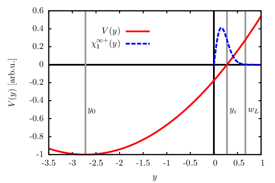
The transverse mode wave functions , which are zero at the boundaries and , satisfy the generalized orthogonality condition[42, 43]
| (26) |
where the modes have been normalized to carry unit flux, so that the scattering matrix is unitary.
We now assume that we have an incoming (right-moving) wave in the th mode in the left lead. The wave functions in the left lead and in the right lead are given by
| (27) | ||||
| (28) | ||||
| where | ||||
| (29) | ||||
The continuity condition for the wave functions at demands that
| (30) | ||||
| and | ||||
| (31) | ||||
In order to extract , we multiply Eq. 30 by , add to it times Eq. 31, multiply this equation by , and integrate from to . The right hand side reduces to the generalized orthogonality relation (26) for the transverse wave functions in the lead and therefore simplifies to ,
| (32) |
with being the generalized overlap integral between mode in the left lead and mode in the right lead,
| (33) |
where is the smaller of the two lead widths , . For sufficiently high magnetic field and Fermi momentum , the wave functions in the th mode are small at the upper boundary, so that we expect to be almost one. We define its deviation from 1 by
| (34) |
where for two leads corresponds to of the rough wire introduced in the previous subsection.
Inserting Eq. 34 into the unitarity condition
| (35) | ||||
| (36) |
we find that the can be at most . The second term in Eq. 32 approximately corresponds to the orthogonality condition (26) for , so that it is strongly suppressed. The integrals can be estimated to be of order by using that the difference between the th modes on the left and right side is of order , while the left-moving modes are of order at the upper side of the wire, where differs from . Utilizing that the integral and are both , the whole term should be of order , such that a priori it cannot be neglected. Numerically, we find that its magnitude does not exceed , quite independently of the Fermi energy and the magnetic field . We neglect the second term in Eq. 32 in the following, keeping in mind that this will introduce an error of about in our result for the localization lengths.
We thus approximate
| (37) |
which is independent of the order of the leads. Without loss of generality, we can choose for the further calculation. Since the th mode in the (wider) right lead is much less affected by the upper boundary than the th mode in the (narrower) left lead, we replace the former by the wave function of the th mode in an infinitely wide lead,
| (38) |
The transverse wave function of the th mode in the left lead differs from this only very slightly, see Fig. 12, so we write it as
| (39) |
where is negligible except near and is given by for , where . The normalization factor is close to one and will be evaluated below. The longitudinal momentum in the left lead can be written as
| (40) |
The difference is very small and is numerically found to be .

Inserting (38-40) into Eq. 37 and extending the integral to (considering that the wave function is zero for ), we have
| (41) |
and thus
| (42) |
with
| (43) | ||||
| (44) |
To calculate , we use the flux normalization condition from Eq. 26,
| (45) |
which we write as
| (46) |
with
| (47) | ||||
| (48) |
Inserting into Eq. 42, we obtain
| (49) | ||||
| (50) |
where we used that the integrals are much smaller than one. With the explicit expressions for and , the last term becomes
| (51) |
which is of higher order than integral since is almost zero where the wave function has its maximum and is already . Dropping this term, we arrive at a simple expression for ,
| (52) |
A.2.1 WKB approximation of
To evaluate Eq. 52, we need an expression for the function , see Fig. 12. By inserting Eq. 39 into Eq. 25 and imposing the boundary conditions , we find that has to be an eigenfunction of the same Hamiltonian as , but with boundary conditions . Instead of a normalization condition, it has to satisfy . Since the upper boundary is already deep in the classically forbidden region, we use a WKB approximation for our solution for ,
| (53) |
with
| (54) |
where we have used that the effective 1D Schrödinger equation has eigenvalue and the effective potential depends on the longitudinal wave number (cf. Eq. 25). Inserting the above expression into Eq. 52, we find
| (55) |
We extend the first integral to start at and perform in the first integral the substitutions , and , in the second. Since the integrals will only give a significant contribution near , i.e., , we expand into a Taylor series to first order,
| (56) |
Defining , and , we find
| (57) |
Expanding the term in square brackets in powers of gives
| (58) |
Dropping the quadratic term, the evaluation of the integral leads to
| (59) |
with and both evaluated at .
A.2.2 WKB approximation of modes
The next step in our calculation of , and, ultimately, of the mode localization length , is to find an expression for the value of the transverse wave function at the upper boundary and for the longitudinal momentum eigenvalue .
To do this, we rewrite the effective transverse Hamiltonian , following from Eq. 25,
| (60) |
with the potential
| (61) |
with the classical turning point , where the potential value equals the energy . We linearize the potential near the classical turning point (where the WKB solution diverges), which makes it possible to solve the effective Schrödinger equation analytically. The complete wave function is constructed by connecting the solution of the linearized potential near the classical turning point to the WKB solution in the classically forbidden region.
The linearized Schrödinger equation is solved by the Airy function with . The boundary condition at the lower wall demands that is equal to zero, so that must be a zero of . For the solution for the th mode, we choose the th zero at , so that the wave function has nodes. From this follows that
| (62) | ||||
| and by using we find | ||||
| (63) | ||||
For large the longitudinal momentum of the th mode is only marginally smaller than the Fermi momentum (remember that is negative). The maximum of the th transverse mode is between and , i.e., between and . Since approaches for large , the wave function stays closer and closer to the lower wall with increasing .
The transverse wave function near the classical turning point can now be written as
| (64) |
We will construct the full solution for the wave function by using the Airy function near the classical turning point and the WKB solution (which takes the quadratic potential into account) in the classically forbidden region. Before proceeding, we determine the prefactor . Since the WKB solution is only used in describing the exponential tail for , calculating with the wave function of the linearized potential will only introduce a small error. Therefore, we insert Eq. 64 into the flux normalization condition Eq. 26 and obtain
| (65) |
which results in
| (66) |
where and . In the limit of large , this simplifies to
| (67) |
Since we need to evaluate the transverse wave function at , which is deep in the classically forbidden region, we proceed by connecting the Airy function (valid near the classical turning point) to the WKB solution (valid in the classically forbidden region). We write the WKB solution as
| (68) |
and from a short calculation we obtain that the two constants and are related by
| (69) |
For evaluating the integral in Eq. 68, we insert the explicit form of the potential, use as the upper limit of integration, and rewrite Eq. 54 as
| (70) |
leading to
| (71) |
with . We evaluate the above integral by expanding the integrand in powers of ,
| (72) |
Inserting this into Eq. 68, and using that in the limit of large , we obtain
| (73) |
neglecting higher order terms.
A.3 Semiclassical limit with constant cyclotron radius
To obtain our final result for the mode localization length in the semiclassical limit of large , we insert Eq. 74 with into the expression Eq. 24 for . We keep the cyclotron radius constant, such that the classical dynamics is independent of . We expand the prefactor in powers of for , keeping the first two terms in the expansion since they are of similar magnitude for the parameter values used, and finally obtain
| (76) |
where and the dimensionless parameters , , , and are given by
| (77a) | ||||
| (77b) | ||||
| (77c) | ||||
| (77d) | ||||
where we have introduced the dimensionless parameters and . Note that the factor determining the asymptotic exponential behavior does not depend on the mode number . For and in the limit this corresponds to the result we have previously reported.[31]
A.4 Semiclassical limit with constant magnetic field
Instead of keeping the cyclotron radius fixed, we alternatively set the magnetic field to a fixed value independent of and again perform the limit . We repeat the above procedure, introducing the magnetic length through and the dimensionless parameter . As above, we use and obtain
| (78) |
with the dimensionless parameters , , , now given by
| (79a) | ||||
| (79b) | ||||
| (79c) | ||||
| (79d) | ||||
References
- [1] M. C. Gutzwiller, Chaos in Classical and Quantum Mechanics (Interdisciplinary Applied Mathematics) (v. 1) (Springer, 1991), 1st ed., ISBN 0387971734.
- [2] L. Markus and K. R. Meyer, Generic Hamiltonian Dynamical Systems Are Neither Integrable Nor Ergodic (Memoirs of the American Mathematical Society) (American Mathematical Society, 1974), ISBN 0821818449.
- [3] K. B. Efetov, Phys. Rev. Lett. 79, 491 (1997).
- [4] S. Flach, O. Yevtushenko, and Y. Zolotaryuk, Phys. Rev. Lett. 84, 2358 (2000).
- [5] H. Schanz, M. F. Otto, R. Ketzmerick, and T. Dittrich, Phys. Rev. Lett. 87, 070601 (2001); H. Schanz, T. Dittrich, and R. Ketzmerick, Phys. Rev. E 71, 026228 (2005).
- [6] M. Prusty and H. Schanz, Phys. Rev. Lett. 96, 130601 (2006).
- [7] H. Schanz and M. Prusty, J. Phys. A 38, 10085 (2005).
- [8] M. J. Davis and E. J. Heller, J. Chem. Phys. 75, 246 (1981).
- [9] J. D. Hanson, E. Ott, and T. M. Antonsen, Phys. Rev. A 29, 819 (1984).
- [10] S. Fishman, I. Guarneri, and L. Rebuzzini, Phys. Rev. Lett. 89, 084101 (2002).
- [11] L. Hufnagel, R. Ketzmerick, M.-F. Otto, and H. Schanz, Phys. Rev. Lett. 89, 154101 (2002).
- [12] A. Iomin, S. Fishman, and G. M. Zaslavsky, Phys. Rev. E 65, 036215 (2002).
- [13] A. Bäcker, R. Ketzmerick, and A. G. Monastra, Phys. Rev. Lett. 94, 054102 (2005); A. Bäcker, R. Ketzmerick, and A. G. Monastra, Phys. Rev. E 75, 066204 (2007).
- [14] S. Tomsovic and D. Ullmo, Phys. Rev. E 50, 145 (1994); O. Bohigas, S. Tomsovic, and D. Ullmo, Physics Reports 223, 43 (1993).
- [15] V. A. Podolskiy and E. E. Narimanov, Phys. Rev. Lett. 91, 263601 (2003).
- [16] A. Bäcker, R. Ketzmerick, S. Löck, and L. Schilling, Phys. Rev. Lett. 100, 104101 (2008a).
- [17] A. Bäcker, R. Ketzmerick, S. Löck, M. Robnik, G. Vidmar, R. Höhmann, U. Kuhl, and H. J. Stöckmann, Phys. Rev. Lett. 100, 174103 (2008b).
- [18] W. K. Hensinger, H. Haffner, A. Browaeys, N. R. Heckenberg, K. Helmerson, C. Mckenzie, G. J. Milburn, W. D. Phillips, S. L. Rolston, H. Rubinsztein-Dunlop, et al., Nature 412, 52 (2001).
- [19] D. A. Steck, W. H. Oskay, and M. G. Raizen, Science 293, 274 (2001).
- [20] M. Leadbeater, V. I. Falko, and C. J. Lambert, Phys. Rev. Lett. 81, 1274 (1998).
- [21] J. A. Sánchez-Gil, V. Freilikher, A. A. Maradudin, and I. V. Yurkevich, Phys. Rev. B 59, 5915 (1999).
- [22] A. García-Martín and J. J. Sáenz, Phys. Rev. Lett. 87, 116603 (2001).
- [23] A. García-Martín, M. Governale, and P. Wölfle, Phys. Rev. B 66, 233307 (2002).
- [24] F. M. Izrailev, J. A. Méndez-Bermúdez, and G. A. Luna-Acosta, Phys. Rev. E 68, 066201 (2003).
- [25] E. I. Chaikina, S. Stepanov, A. G. Navarrete, E. R. Méndez, and T. A. Leskova, Phys. Rev. B 71, 085419 (2005).
- [26] Q. Song, L. Wang, S. Xiao, X. Zhou, L. Liu, and L. Xu, Phys. Rev. B 72, 035424 (2005).
- [27] U. Kuhl, F. M. Izrailev, and A. A. Krokhin, Phys. Rev. Lett. 100, 126402 (2008).
- [28] W.-K. Hong, J. I. Sohn, D.-K. Hwang, S.-S. Kwon, G. Jo, S. Song, S.-M. Kim, H.-J. Ko, S.-J. Park, M. E. Welland, et al., Nano Letters 8, 950 (2008).
- [29] M. Evaldsson, I. V. Zozoulenko, H. Xu, and T. Heinzel, Phys. Rev. B 78, 161407(R) (2008).
- [30] E. R. Mucciolo, A. H. Castro Neto, and C. H. Lewenkopf, Phys. Rev. B 79, 075407 (2009).
- [31] J. Feist, A. Bäcker, R. Ketzmerick, S. Rotter, B. Huckestein, and J. Burgdörfer, Phys. Rev. Lett. 97, 116804 (2006).
- [32] A. M. Kosevich and I. M. Lifshitz, Zh. Eksp. Teor. Fiz. 29, 743 (1955).
- [33] C. W. J. Beenakker and H. van Houten, Phys. Rev. Lett. 60, 2406 (1988).
- [34] A. Bäcker, A. Manze, B. Huckestein, and R. Ketzmerick, Phys. Rev. E 66, 016211 (2002).
- [35] B. Weingartner, S. Rotter, and J. Burgdörfer, Phys. Rev. B 72, 115342 (2005); A. Bäcker, S. Fürstberger, and R. Schubert, Phys. Rev. E 70, 036204 (2004).
- [36] S. Rotter, J. Z. Tang, L. Wirtz, J. Trost, and J. Burgdörfer, Phys. Rev. B 62, 1950 (2000).
- [37] S. Rotter, B. Weingartner, N. Rohringer, and J. Burgdörfer, Phys. Rev. B 68, 165302 (2003).
- [38] J. Skjånes, E. H. Hauge, and G. Schön, Phys. Rev. B 50, 8636 (1994).
- [39] L. Onsager, Phys. Rev. 38, 2265 (1931).
- [40] H. B. G. Casimir, Rev. Mod. Phys 17, 343 (1945).
- [41] M. Büttiker, Phys. Rev. Lett. 57, 1761 (1986).
- [42] H. U. Baranger and A. D. Stone, Phys. Rev. B 40, 8169 (1989).
- [43] R. L. Schult, H. W. Wyld, and D. G. Ravenhall, Phys. Rev. B 41, 12760 (1990).