Axigluon Couplings in the Presence of Extra Color-Octet Spin-One Fields
Abstract
In this paper, we study how the interaction of the axigluon with quarks is modified when we introduce new color-octet spin-one fields in a chiral color model. We show that in this case the strength of this interaction is not completely determined by the gauge symmetry any more and can be significantly weaker than the one predicted in the original chiral color model. In this way, we reinterpret the non-observability of the axigluon at the Tevatron, not as a limit on the axigluon mass, but as a limit on the strength of the axigluon coupling to quarks.
1 Introduction
It is inherent to science to look forward to new horizons and explore every possible path in the hope to increase our knowledge about Nature. That’s why, despite the amazing phenomenological success of the Standard Model, we are always tempted to extend its particle content or its symmetry and study the properties of the resulting model. Of course there are good theoretical reasons for doing it: we need to explain many mysteries present in the foundations of the Standard Model. Perhaps the best known example is the problem of naturalness in the Higgs sector. The necessity of understanding why we observe a so large hierarchy between the electroweak scale and, for example, the Grand Unification scale, have motivated the construction of models as different as supersymmetry, Technicolor or Little Higgs, among others. In all these theories, the hierarchy problem is solved at the price of significantly extend the particle and symmetry contents proposed by the Standard Model and verified to the level of 1% at LEP.
Another intriguing, but much less popular, question is why we observe a so different structure for the weak and strong interactions. The weak interaction is profoundly chiral while the strong interaction makes no difference between left and right fermions. In this context, and with the aim of unification in their eyes, Frampton and Glashow [1, 2] proposed many years ago a family of models where the local gauge symmetry of the strong interaction is supposed to be at high energies. Of course at some large energy scale this symmetry must be broken to its diagonal group which is identified with the usual QCD group: . A general prediction of this kind of models is the existence of a massive color-octet spin-one particle usually called axigluon because it has an axial coupling to quarks. The strength of this coupling is, as we will see, completely dictated by the gauge symmetry and, in the simplest, model is equal to the gluon-quark interaction. Of course the presence of such a particle would introduce a large contribution in the dijet production cross section at hadron colliders. Unfortunately, such a signal has not been observed and stringent limits have been placed on the axigluon mass [3]. Phenomenological constrains have also been obtained from top-antitop events [4].
In this paper, we study how the interaction of the axigluon with quarks is modified when we introduce new color-octet spin-one fields. We will show that in this case the strength of this interaction is not completely determined by the gauge symmetry any more and can be significantly weaker than the one predicted in the original chiral color model. In this way we can reinterpret the non-observability of the axigluon at the Tevatron not as a limit on the axigluon mass, but as a limit on the strength of the axigluon coupling to quarks.
2 Chiral Color and the Axigluon
We start by recalling the origin of the axigluon in chiral color models. Of course, this revision will be schematic and we will not discuss important points such as the choise of anomaly free representations for fermions11 1 A detailed discussion of this topics can be found in [1], [2] and [5]. We will concentrate only in those aspects we judge important for the axigluon phenomenology.
Let us, then, consider the following Lagrangian:
| (1) |
where
and () is the gauge field of (). Of course, the first two terms are invariant under transformations and the third term is a nonlinear sigma model term we include to describe the breaking down of the original local gauge symmetry to . Although it is straightforward to develop the model considering different coupling constants for and [6] we are going to limit ourselves to the case where . We do it in order to simplify our analysis and because this was the choice made by authors of the original chiral color model motivated by unification arguments[1].
In the unitary gauge (), the third term of equation (1) gives rise to a nondiagonal mass matrix for the gauge bosons.When we diagonalize the mass matrix, we found the following eigenvalues and eigenvectors:
| (2) | |||||
| (3) |
where is the gluon and is the axigluon.
The interaction Lagrangian for the quarks can be written as:
| (4) |
Inverting equations (2) and (3) we can write the Lagrangian in term of the physical fields and we obtain:
| (5) |
In this minimal model, the gluon-quark and axigluon-quark interaction terms have the same coupling constant . In more general models, where , it is not true and appears modulated by trigonometric functions of a mixing angle[6].
3 Our Model
Following the ideas previously developed by the author in [7] and [8], we propose to modify the model described above by adding new spin-one fields, and , which transform like gauge fields under and respectively with a characteristic coupling constant . The Lagrangian that describes the gauge sector of the model, including the effective symmetry breaking term, is
| (6) | |||||
where , and are the same than in the previous section while and are defined by
Again, in the unitary gauge a nondiagonal mass matrix is explicitly generated. Although the resulting mass matrix can be exactly diagonalized, in order to obtain easily manipulable expressions we will assume that and we will write our results in the first order in . The eigenvalues, that is, the masses of the physical states are:
Thus, the physical spectrum is composed of a (exactly) massless gluon, an axigluon with the same mass (in this limit) than in the minimal model and two degenerate (at this level of approximation) heavy gluon and axigluon. Notice that the new mass scale is not constrained and we can safely suppose that it is large enough to prevent the observation of the heavy states.
The normalized mass eigenvectors can be written as:
| (7) | |||||
Because we have now two fields that transform as gauge fields for each group ( and for and and for ) any combination of the form and , where and are arbitrary constants, can be used to construct covariant derivatives[7]. This means that the Lagrangian describing the gauge interaction of quarks can be written as:
| (8) | |||||
In principle, and are independent parameters but, again, for simplicity we will assume that . Using Lagrangian (8) and the definition of the physical fields, we can obtain the terms of the Lagrangian that couple the gluon and the axigluon to quarks
| (9) |
where is defined as:
| (10) |
Notice that, while the coupling of the gluon to the quarks is the usual one and is independent of (because is protected by the gauge symmetry), the coupling constant of the axigluon has been modified and now depend on the free parameter . Of course we can use this freedom to choice an adequated valued in order to make the axigluon invisible at the Tevatron.
Let us briefly comment about to keep and as independent parameters. In this case, additionally to the axial coupling, a new vector coupling would appear between the axigluon and the quarks, proportional to .
4 Results
Now we want to estimate the values of allowed by experiments. It is evident that, in order to keep the axigluon invisible in dijet observations at the Tevatron, the following inequality must be satisfied:
| (11) |
where is the maximum value of the production cross section of a resonance decaying into dijets, allowed by experiment at 95% C.L. and is the cross section for the production of an axigluon and its decay into dijets in the usual minimal model ().
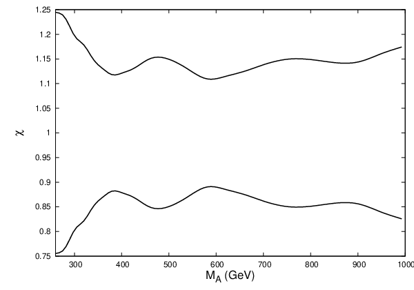
We use Calchep [9] in order to estimate for TeV, and (where is the rapidity of the jet) for values of the axigluon mass in the interval GeV. For , we use the values reported in [3].
The results are summarized in figure 1. The continuous curves represent the limits on obtained using the equality in (11). The allowed region is the one between the curves. For , the axigluon completely decouple from quarks but, we can see, a deviation of from of about is allowed for the whole mass range considered here. But for low masses a deviation as large as is still possible.
5 Conclusion
In this work we have presented a new mechanism to reduce the coupling of the axigluon to quarks in order to evade the limits imposed by dijet production experiments. This mechanism consists in adding new spin-one fields that originally transform like gauge fields under and respectively and construct with them generalized covariant derivatives. We want to emphasize that our method is rather innocuous. Our model preserve the fundamental structure of chiral color models and from equation (7) we can see that the descomposition of the physical states in terms of the original has the same structure for the light fields (the gluon and the axigluon) and the heavy ones. That implies that their interaction to quarks has also the same structure. Thus, we expect that once one has chosen anomaly free representations for quarks in the minimal model, the potentially new anomalous diagrams introduced in our model by the heavy states will also cancel. On the other hand, although we have shown that our proposal works in the important case where we keep the symmetry between the left and right sectors, it is straightforward to generalize it to the case when . In this case, we can reduce independently the axial as well as the vector coupling that the axigluon develops in this generalized models. For doing that, it is enough to keep in equation (8). Finally, the appearance of a heavy gluon and a heavy axigluon is not problematic from a phenomenological point of view since the model allows their mass to be large enough to be invisible at the Tevatron.
Acknowledgement
A. R. Z. is partially supported by Fondecyt grant 1070880. The author wants to thank the hospitality of the Instituto de Física Teórica (Unesp), São Paulo, Brazil, where this work was completed.TGD
References
- [1] P. H. Frampton and S. L. Glashow, “Unifiable Chiral Color With Natural Gim Mechanism,” Phys. Rev. Lett. 58 (1987) 2168.
- [2] P. H. Frampton and S. L. Glashow, “Chiral Color: An Alternative to the Standard Model,” Phys. Lett. B 190 (1987) 157.
- [3] T. Aaltonen et al. [CDF Collaboration], “Search for new particles decaying into dijets in proton-antiproton collisions at sqrt(s) = 1.96 TeV,” Phys. Rev. D 79 (2009) 112002 [arXiv:0812.4036 [hep-ex]].
- [4] P. Ferrario and G. Rodrigo, “Constraining heavy colored resonances from top-antitop quark events,” arXiv:0906.5541 [hep-ph].
- [5] P. H. Frampton, “Gauge Field Theory”, John Wiley & Sons, INC, 2000, second edition.
- [6] M. V. Martynov and A. D. Smirnov, “Chiral color symmetry and possible -boson effects at the Tevatron and LHC,” arXiv:0906.4525 [hep-ph].
- [7] A. R. Zerwekh, “Effective description of a gauge field and a tower of massive vector resonances,” arXiv:hep-ph/0307130.
- [8] A. R. Zerwekh, “Consequences of partial vector meson dominance for the phenomenology of colored technihadrons,” Eur. Phys. J. C 49, 1077 (2007) [arXiv:hep-ph/0603094].
- [9] A. Pukhov, arXiv:hep-ph/0412191.