The LCFIVertex package: vertexing, flavour tagging and vertex charge reconstruction with an ILC vertex detector
Abstract
The precision measurements envisaged at the International Linear Collider (ILC) depend on excellent instrumentation and reconstruction software. The correct identification of heavy flavour jets, placing unprecedented requirements on the quality of the vertex detector, will be central for the ILC programme. This paper describes the LCFIVertex software, which provides tools for vertex finding and for identification of the flavour and charge of the leading hadron in heavy flavour jets. These tools are essential for the ongoing optimisation of the vertex detector design for linear colliders such as the ILC. The paper describes the algorithms implemented in the LCFIVertex package, as well as the scope of the code and its performance for a typical vertex detector design.
Keywords:
Simulation , Reconstruction , Monte Carlo , Software tools , Vertex detectors , Linear colliderPACS
29.85.Fj , 07.05.Tp , 07.05.Fb , 29.40.Gx , 23.70.+j , 07.05.Mh, , , , , , , , , , , , , , , , , , , , , , , , , , , , , , , , , , , , , , , , , , , , , , , , , , , , , , , , , ,
1 Introduction
1.1 Purpose and scope of the LCFIVertex package
The International Linear Collider (ILC), colliding electrons and positrons, is envisaged by the particle physics community to be the next high energy accelerator for particle physics research. Its centre of mass energy is planned to initially range from for physics runs and down to for calibration purposes, with the possibility of a later upgrade to [1]. The ILC with its well-known momentum and spin state of the interacting particles will be complementary to the Large Hadron Collider (LHC), providing capability of precise measurements of new physics phenomena and indirect studies of phenomena at energy scales well beyond the direct energy reach of both the ILC and LHC [2]. Overviews of the physics accessible at the ILC are given in the TESLA Technical Design Report [2] and in the ILC Reference Design Report [1]. The complementarity of the ILC and the LHC has been investigated in detail by the LHC/ILC Study Group [3].
Extraction of new physics accessible at the ILC will rely not only on high quality of the colliding beams, but also on the use of hermetic, high-precision detector systems to record the signals of the products of the collisions, as well as excellent reconstruction software to analyse these events. Since ILC physics is expected to be rich in final states with heavy flavour jets, it will be important to be able to distinguish jets, for which the leading hadron contains a bottom valence quark, from jets containing hadrons with a charm valence quark and jets arising from light (, , ) quark hadronisation. Crucial for this “flavour tag” is the high precision measurement of the tracks of charged particles in the innermost detector system, the vertex detector, permitting reconstruction of the decay vertices of heavy flavour hadrons. As shown at previous experiments, a sufficiently precise and mechanically stable detector permits the reconstruction of both the primary vertex at the point where the particle beams collide, and the full decay chain in heavy flavour jets. For example, in a typical jet containing a hadron decay away from the interaction point (IP), resulting in a hadron that decays, e.g., further away, it is often possible to reconstruct all three vertices from the tracks in the jet. Jet flavour identification is aided by observables derived from these vertices, such as the mass and momentum of the leading hadron that decayed. Further, measurement of the vertex charge permits one to determine if the heavy flavour parton is a quark or an antiquark, opening up a range of measurements that would otherwise be inaccessible.
The LCFIVertex package provides software for vertex finding, flavour tagging and vertex charge reconstruction. In the current phase of ILC detector research and development, the code is intended for the optimisation of the vertex detector design. Furthermore, it is currently being used for optimisation of the overall ILC detector concepts, which requires flavour tagging in order to study the benchmark physics processes chosen to assess the performance of different detector designs.
This paper describes the functionality provided by the LCFIVertex package, as well as the performance achieved for a typical ILC vertex detector design. Emphasis is on the algorithms; further technical information can be found in the software documentation [4]. The paper is structured as follows: the vertex detector design used for the performance examples and the software framework to which the LCFIVertex code is interfaced are described in the remainder of this section. Section 2 describes the track selection used for the different parts of the code; in particular, the algorithms to suppress tracks stemming from photon conversions in the tracking volume and from the decay of short-lived and hadrons are described. Section 3 explains the vertex finding algorithms, Section 4 the flavour tag and neural net software on which the flavour tagging approach relies and Section 5 the algorithm for quark charge reconstruction. Examples of the resulting performance for a typical detector design, using a sample of with at a centre-of-mass energy , unless otherwise stated, are presented in addition to the algorithms. Section 6 gives a summary of the paper. Software versions and parameter settings used to produce the results in this paper are described in Appendices A–C.
1.2 The detector design used for performance evaluation
The results presented in this paper were obtained with the detector
model LDCPrime_02Sc [5].
This detector design evolved from the earlier TESLA detector geometry
[2] and was implemented in a Geant4-based detector
simulation by the LDC (“Large Detector Concept”) study group.
It relies mostly on a pixel-based silicon vertex detector and a time projection
chamber (TPC) to provide charged particle tracking.
These detectors are located inside a solenoid which provides a
magnetic field of .
Also inside the solenoid are fine grained electromagnetic (ECAL) and
hadronic (HCAL) calorimeters.
Additional tracking and calorimetry is foreseen in the forward region,
which is particularly important at ILC energies, given that many of the
relevant physics processes are expected to give rise to multi-jet final
states with at least one jet in the forward direction. The tracking detector layout
of the LDCPrime_02Sc detector model is shown in Figure 1.
The vertex detector geometry in LDCPrime_02Sc consists of five
barrel layers of silicon sensors evenly spaced between the inner
radius of and the outer radius of .
The length of the active area is for the outer four
layers and for the innermost layer. The number of
sensor staves per layer ranges between and . Sensors are
assumed to be mounted onto a carbon fibre support structure, with the
combined material budget of sensor and support structure corresponding
to of a radiation length per layer. As carbon fibre is not
among the materials available in Geant, the support is described as a
thick layer of graphite in the simulation. At
the ends of the barrel staves, the amount of material is larger due to
the electronics and mechanical fixtures needed. In the barrel region,
the silicon intermediate tracker (SIT), consisting of two layers of
silicon sensors located at radii and
, respectively, helps link the track segments
measured in the vertex detector to those provided by the TPC. In the
detector design considered, the TPC drift region has an inner radius
of , an outer radius of and a
half-length of . In the forward direction,
tracking is complemented by a silicon strip detector, the forward
track detector (FTD), comprised of disks located at positions
ranging from to with inner
radii between and and outer
radii between and . The inner
radius of the silicon-tungsten ECAL is and its
outer radius is . The ECAL is surrounded by an
iron-scintillator HCAL with an inner radius of .
Calorimeter cells are squares with sides of length in
the ECAL and in the HCAL. In the forward region, an
ECAL endcap extends from to , followed by an HCAL from .
1.3 LCIO data format and the MarlinReco software framework
The results presented in this paper were obtained with input from
the Pythia event generator [6].
The detector response was simulated using the Geant4-based
[7] program MOKKA [8]
and the detector model LDCPrime_02Sc, described above.
The Linear Collider I/O (LCIO) persistency framework [9]
permits storage of results between the stages of detector simulation,
event reconstruction and physics analysis, and the exchange of these
results between the different software frameworks used for ILC
detector optimisation.
One of the main roles of LCIO is to provide a common data model,
in which an Event entity holds collections of objects relevant
to the different stages of reconstruction, as well as some of the
Monte Carlo (MC) information from the event generator.
Reconstruction was performed using tools from the MarlinReco event reconstruction package [10], based on the particle flow concept and implemented within the modular C++ application framework Marlin [11]. The modules are called “processors” in this framework and can be configured by steering files in xml format.
Specific MarlinReco processors were used to simulate the digitization
in the different detector subsystems.
In the case of the silicon-based detectors, the physical processes
occurring in the silicon sensors, such as the drift of the electrons
and holes that give rise to the signals, are described using simple
parameterisations.
Track finding, including pattern recognition, and track fitting was
then performed using the FullLDCTracking processor
[12, 13].
Calorimeter clusters and tracks are matched using a particle flow
algorithm (PFA).
For this purpose, the PandoraPFA code [14]
was used, resulting in a collection of ReconstructedParticles.
These are the entities in LCIO on which analyses are usually based,
and which are used, for example, as the input to jet finding
algorithms.
The LCFIVertex code is run on jets, and hence for studies in the
context of PFA-oriented detectors, like the one described here,
requires the PFA code to be run before the jet finding step.
Calorimeter clusters are required by the PFA algorithm as part of
the input, and therefore also need to be reconstructed before this
algorithm can be run.
Via the jet energy, calculated in the PFA code, calorimeter clusters
are indirectly used for the flavour tag.
Otherwise, the LCFIVertex code is independent of the calorimeter
information and only accesses the tracks in the input jets.
It was checked that when running a different particle flow
algorithm available in MarlinReco, Wolf [15],
flavour tagging performance did not change.
The Durham -cluster jet finding algorithm, as implemented in
the SatoruJetFinder package in MarlinReco [16],
was then run, forcing each event into a two-jet topology.
Tracks from photon conversions, and decays were
identified by a conversion tagger that forms part of LCFIVertex,
see Section 2.1.
These tracks were excluded from the input passed to the LCFIVertex
processors.
A simple processor to determine the event vertex or interaction point (IP) from an iterative fit to a subset of all tracks in an event was run. This IP-fit processor and the conversion tagger are the only parts of the LCFIVertex package that are not jet-based. The resulting event vertex is used both by the vertex finding algorithms described below and for the flavour tag to determine a track’s point of closest approach to the IP.
2 Track Selection
The default flavour tag procedure implemented in the LCFIVertex package, as described in more detail in Section 4, uses secondary vertex information whenever available. Different neural networks with separate sets of input variables are used depending on whether secondary vertices are found or not. In particular, for distinguishing jets from jets, a useful criterion is that jets do not contain vertices stemming from the decays of heavy flavour hadrons. It must therefore be ensured that the vertex finder creates as few fake vertices from wrong track combinations as possible. This can partly be achieved by appropriate track selection, as discussed in Section 2.1. Other potential sources of unwanted vertices for the purpose of flavour tagging are photon conversions in the detector material and the decay of and particles, which can resemble a heavy flavour decay vertex. As these effects have clear signatures, such tracks can easily be identified and suppressed by the track selection.
2.1 Identification of tracks from photon conversions, and decays
A dedicated Marlin processor is used to identify tracks from and decays and from photon conversions. All two-track combinations are considered as candidates and are required to pass the following criteria to be identified as conversions or / decays:
- •
The constituent tracks must have opposite charge sign.
- •
The distance of closest approach between the two track helices must not exceed .
- •
The distance between the point of closest approach and the IP must be larger than in order to reduce the risk of fake tags consisting of combinations of primary vertex tracks.
- •
The invariant mass of the two track combination has to be compatible with that of the photon, the or the .
To check the mass compatibility, the rest mass of the combination is calculated using three mass hypotheses, choosing the masses of the decay products accordingly: both tracks are assumed to be electrons in the case of conversions, or pions for the hypothesis, and for the hypothesis, the track with larger momentum is assigned the proton mass and the other the pion mass. The resulting rest mass of the combination is considered to be compatible with the hypothesis if it differs from the PDG value by not more than for conversions and Kaons and by not more than for Lambdas. Table 1 lists performance figures for each particle type separately.
| particle | efficiency | purity |
|---|---|---|
| photon | 24.6% | 96.3% |
| 72.2% | 67.4% | |
| 69.8% | 62.3% |
All objects that are not identified as stemming from the above sources are passed on to the track selection processor preceding the subsequent steps such as vertex finding and flavour tagging.
In addition to this core functionality, the conversion tagger can also be run in one of two “cheater” modes, which use MC information to identify conversions and or decays and can be used to assess the performance of the realistic reconstruction. The two cheater modes differ in the way they treat the case that only one of the tracks from a conversion or / decay has been reconstructed, the other track not being within the detector acceptance or being lost due to pattern recognition inefficiencies. The more moderate cheater mode then does not flag the track that could be reconstructed as resulting from a conversion or / decay, since no realistic algorithm could possibly identify such tracks, whereas the more aggressive cheater mode flags all tracks that stem from these sources.
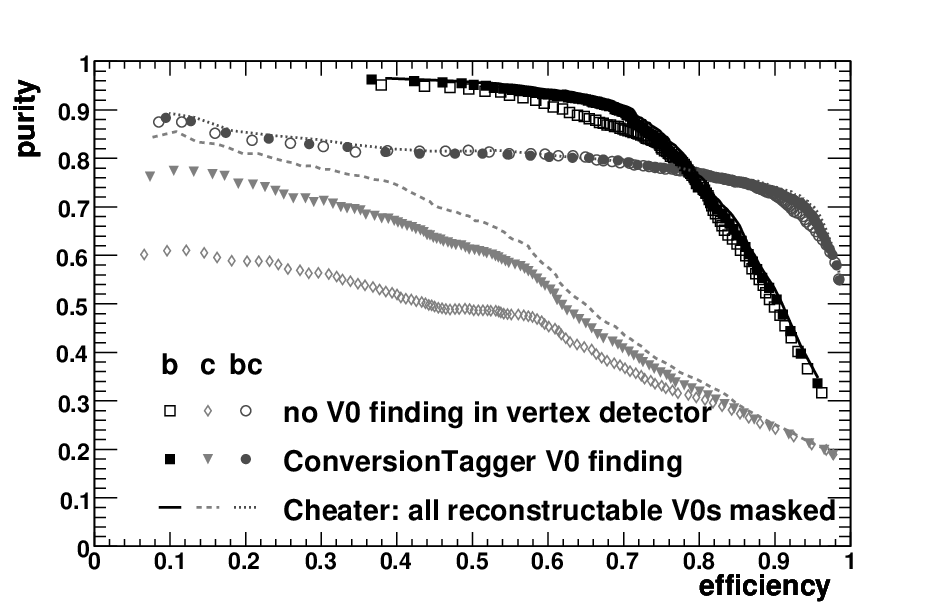
Figure 2 shows the flavour tagging performance in terms of purity vs. efficiency for the three tags provided (see Section 4.3 for details) when the conversion tagger is run as part of the reconstruction chain (full symbols). Performance without any / identification and with only the conversions that PandoraPFA finds removed, i.e. no conversion finding in the vertex detector, is plotted for comparison (open symbols). Also shown is the performance obtained from the moderate cheater mode (lines).
2.2 Track selection for IP fit, ZVTOP and flavour tag
| parameter | IP fit | vertexing (ZVRES) | flavour tag |
| of track fit | 5 | 4 | — |
| - impact parameter (mm) | 20 | 2 | 20 |
| uncertainty (mm) | — | 0.007 | — |
| impact parameter (mm) | 20 | 5 | 20 |
| uncertainty (mm) | — | 0.025 | — |
| track () | 0.1 | 0.2 | 0.1 |
The track selection can be tuned separately for the IP fit, the ZVTOP vertex finder and the calculation of the flavour tag inputs. An overview of the track selection cuts for each of these tasks is given in Table 2. In addition to the cuts listed in the table, requirements are implemented on the number of hits in the tracking subdetectors as follows: if there are at least hits in the TPC or at least three hits in the FTD, no hit is required in the vertex detector. If there are fewer hits in the TPC or FTD, at least three vertex detector hits are needed.
3 The ZVTOP vertex finding algorithms
The LCFIVertex package contains a complete re-implementation of the topological vertex finder ZVTOP originally developed at the SLD experiment [17]. A modified version of the original Fortran code was used in previous Linear Collider studies, see e.g. Refs. [1, 2]. For the most part, the vertex finding algorithm in LCFIVertex, as described below in this section, corresponds to the original SLD version. Minor improvements of the LCFIVertex algorithm with respect to SLD include a Kalman vertex fit and adjustments to allow use of ZVTOP in events at centre-of-mass energies above the resonance.
3.1 The ZVRES algorithm
The ZVTOP vertex finder provides two complementary algorithms which use topological information to identify track combinations that are likely to have their origin at a common vertex. The first of these, the ZVRES algorithm, can be used to find multi-pronged secondary vertices with an arbitrary geometrical distribution and hence is most generally applicable provided the detector system has a sufficiently high spatial resolution. The object-oriented implementation of the code that forms part of the LCFIVertex package is described in detail elsewhere [18]. Compared to the original implementation, the new code provides several improvements and adjustments to a collider environment with a variable centre-of-mass energy. The remainder of this section outlines the vertexing algorithms and describes these modifications.
A central idea of the ZVRES algorithm is to describe each track by a probability density function in three-dimensional space and to use these to define a vertex function that yields higher values in the vicinity of true vertex locations and lower values elsewhere, as well as providing a criterion for when two vertex candidates are resolved from each other.
The track functions have a Gaussian profile in the plane normal to the trajectory. With the point of closest approach of track to space point , the track function is defined as:
where is the position covariance matrix of the track at .
In its most basic form, the vertex function is defined as
with the second term ensuring that approaches zero in spatial regions in which only one track contributes significantly to the first term and where hence no vertex should be found.
Optionally, further knowledge on where vertices are more likely to be found can be used to weight the vertex function, thereby suppressing fake vertices and increasing the purity of the vertices found (i.e. the fraction of correctly assigned tracks). Knowledge of the IP position can be used to suppress fake vertices from tracks passing close by each other in the vicinity of the IP. This is accomplished by representing the IP by a contribution
where is the position of the IP and the covariance matrix describing the accuracy with which this position is known. This new term contributes to the vertex function in the same way as the Gaussian probability functions representing the tracks, hence the vertex function is redefined as
This definition ensures that space points close to the IP are less likely to be resolved from each other and that tracks that could otherwise give rise to fake vertices are more likely to be assigned to the primary vertex. In the default configuration of the code, the IP contribution is given a weight of .

Similarly, it is kinematically favoured for heavy hadrons to decay close to the jet axis rather than at large angle from it, which is taken into account by weighting the vertex function outside a cylinder of radius by the factor . In this expression, the angle is defined as shown in Fig. 3 and with being an LCFIVertex parameter which the user can set and the jet energy. The jet energy dependent definition of implemented in LCFIVertex takes into account that jets of higher energy are more collimated.
In addition to indicating likely vertex positions, the other main use of the vertex function is to provide a key criterion for merging candidate vertices in the process of vertex finding: space points and are defined to be resolved from each other if along the straight line connecting these points the vertex function falls below a given fraction of the lower of the values and . Vertices that are not resolved according to this criterion will be referred to as unresolved from each other.
The main challenge of many vertex finders used prior to ZVTOP is the large number of track combinations that need to be considered to determine whether they form a good vertex. In contrast, the ZVRES algorithm uses a bottom-up approach, starting out from all possible two-track combinations and using the vertex function as well as the fit to decide which candidates to keep and to merge.
In the initial step, all two-track and optionally all track-IP combinations are fitted with a Kalman vertex fit. Of these two-object fits, those with lower than a threshold and vertex function at the fitted vertex position above a threshold are retained. Before beginning the merging, the number of remaining two-object fits to be further considered is reduced as follows: for each track in turn, all the two-object combinations that contain the track are considered. The track is removed from all vertices with below of , the maximum vertex function value obtained from the fits for the track under consideration. The track’s two-object fits are sorted with respect to their vertex function . All vertex candidates for which both objects have been removed at this stage are discarded.
The remaining candidate vertices are then merged making further use of the resolvability criterion: starting out from the candidate vertex with the highest vertex function in the sorted list found in the previous step, a set of unresolved vertices is found by iteratively adding other candidates that are unresolved from any of the vertices in the set. The resulting set of unresolved candidate vertices is then merged to form a new candidate. From the remaining vertices, the next seed in the sorted list is picked and the process continues until all original candidate vertices have either been absorbed or considered as seeds for an unresolved set. Note that for the merging phase, the vertex function is not evaluated at the position of the original two-object candidate vertex, but at the closest local maximum of the vertex function, in order to improve the suppression of fake vertices.
Following the merging phase, tracks with a high contribution are removed from the resulting candidate vertices: iteratively, the track with the highest contribution is removed if its is above a threshold . The vertex is refitted and this step is repeated until the highest track passes the cut. Candidates that, after this procedure, are no longer associated with either at least two tracks or with the combination of the IP object and , or more tracks, are discarded.
Remaining ambiguities in the association of tracks to vertices are resolved by keeping each track only in the vertex candidate with highest and removing it from all others. The resulting track combinations are fitted to yield the final vertices, which are sorted with respect to their distance from the IP.
3.2 The ZVKIN algorithm
The ZVTOP vertex finder also provides an algorithm, ZVKIN, to address a particular category of jets for which the ZVRES algorithm fails, namely jets with two subsequent one-prong decays (i.e. decays in which only one charged track is detected), see e.g. Ref. [19] for a description of the algorithm at SLD, and Ref. [18] for further details of the C++ implementation. For cases with one multi-prong vertex and one single-prong vertex a recovery algorithm can identify the decay track and subsequently add it to the decay chain (see Section 4.2 for details). However, if only one charged track can be detected from both the vertex and the vertex, a different approach is needed. The solution chosen in the ZVKIN algorithm is to use additional kinematic information by approximating the direction of flight of the hadron and forming a “ghost track” from it. This ghost track, described as a straight line with an appropriate circular error ellipse of constant width along the track, is added to the set of tracks from which vertices are found. The algorithm consists of two main stages: first the ghost track direction and width are found using an iterative minimisation approach. In the second stage this ghost track is used to constrain the secondary vertex finding.
The jet axis is chosen to initialise the ghost track direction. Fixed at the position of the IP, the ghost track is swivelled in both and directions, until the value
is minimal, where is the of the vertex fit found using track and and , and runs over all input tracks. The value is the distance from the IP to the projection of the vertex onto , with the sign chosen to be positive if the vertex is in the hemisphere defined by the direction of the jet axis. Minimisation continues until changes in both and by do not yield further improvement. If the initial direction of is relatively far from the true line of flight of the hadron, then some, or possibly all, of the secondary tracks will yield a vertex with that has a negative value of . The first minimisation stage is designed so that the contribution to from tracks with will tend to push the ghost track towards the flight path in the minimisation process. The term ensures that the changes in a continuous manner at .
At this point, the width of the ghost track is calculated such that the largest value of for the vertex fit of any of the tracks with is equal to 1. If it is above the user-settable minimum width required for , it is used in the next step; otherwise the minimum width is used. With the adjusted ghost track width, the ghost track direction is further optimised, using the same algorithm as before, but this time minimising the quantity
The width is then adjusted as before. This choice ensures that the corresponding vertex probability has an approximately flat distribution between and , while fake vertices yield values close to 0. The vertex probability is calculated from the value of the vertex fit following the standard algorithm described in [20].
The resulting optimised ghost track is then used to find vertices as follows: from each track in the jet, a vertex is formed with the ghost track. The IP is added to this initial set of vertices. For all possible pairs of vertices from this set, the vertex probability is calculated, omitting the ghost track from the combinations that contain the IP. The pair that maximises this probability is merged and replaces the original vertices in the list. Combinations with vertex probability below a threshold value are not accepted, while the original vertices which formed the combination are separately retained. The merging process continues until no further combination yields a vertex probability above or until there is only one vertex left. Finally, the ghost track is removed from all vertices without refitting them, with the possibility that secondary vertices contain only one track.
3.3 Performance of vertex finding for a typical ILC vertex detector design
All results presented in this section were obtained with the ZVRES algorithm, described in Section 3.1, which applies to a broader class of jets than ZVKIN.
 |
| (a) |
 |
| (b) |
A pure sample of jets from the process at was used, permitting a direct comparison with earlier studies at that energy. Figure 4 (a) shows the probability of the secondary vertex fit. This variable cross-checks the vertex fitter, a reasonably flat distribution, as seen in the figure, indicating that the fitter performs as expected. For a study of the dependence of vertex finding on the decay length of the hadron, a sub-sample was selected, consisting only of jets in which a hadron decayed to a charged hadron, either directly or via a short-lived resonance (with the lifetime being so short that it does not travel any measurable distance in the detector, but decays essentially at its point of origin). The decay lengths of the and the hadron which were chosen in the MC simulation were determined for each jet and compared to the values reconstructed by the ZVRES algorithm. For this comparison the efficiency of finding a secondary vertex within a given decay length interval was plotted as a function of the true MC hadron decay length, as shown in Fig. 4 (b).
 |
 |
| (a) | (b) |
Using the same sub-sample of jets as in Fig. 4 (b), the reconstructed decay lengths of the and hadron were compared to the corresponding MC decay lengths on a jet-by-jet basis. In Fig. 5 (a), the decay length comparison is shown for jets in which at least two vertices (the primary, or IP vertex, plus at least one secondary vertex) were found. This class of jets includes cases in which the hadron decayed so close to the decay vertex that it could not be resolved from it, and for which therefore the reconstructed decay length is shifted to larger values compared to the MC decay length. Short decay lengths, not permitting the decay vertex to be resolved from the primary vertex, also result in deviation of the reconstructed secondary vertex decay length from the MC truth value. In Fig. 5 (b), the decay length of the hadron decay is compared to the MC value for jets in which exactly three vertices were reconstructed by ZVRES. As expected for this category of jets, the correlation between reconstructed and MC values is better.
| Monte Carlo | Reconstructed track-vertex association | |||||||
| track origin | Two vertex case | Three vertex case | ||||||
| pri | sec | iso | pri | sec | ter | iso | ||
| Primary | 91.5 | 1.4 | 36.2 | 95.2 | 3.1 | 1.9 | 49.9 | |
| decay | 6.7 | 46.7 | 29.6 | 3.1 | 75.3 | 10.6 | 22.8 | |
| decay | 1.8 | 51.9 | 34.2 | 1.7 | 21.6 | 87.5 | 27.2 | |
| Primary | 93.7 | 2.6 | 35.3 | 97.4 | 4.9 | 4.0 | 48.5 | |
| decay | 4.6 | 47.3 | 29.8 | 1.8 | 72.3 | 13.5 | 24.5 | |
| decay | 1.7 | 50.1 | 34.9 | 0.8 | 22.9 | 82.5 | 27.0 | |
| Monte Carlo | Reconstructed track-vertex association | |||||||
| track origin | Two vertex case | Three vertex case | ||||||
| pri | sec | iso | pri | sec | ter | iso | ||
| Primary | 95.9 | 6.3 | 77.0 | 96.8 | 30.5 | 29.1 | 77.7 | |
| decay | 4.1 | 93.7 | 23.0 | 3.2 | 69.5 | 70.9 | 22.3 | |
| Primary | 97.5 | 9.0 | 73.1 | 96.7 | 20.2 | 51 | 73.6 | |
| decay | 2.5 | 91.0 | 26.9 | 3.3 | 79.3 | 48.7 | 26.4 | |
| Monte Carlo | Reconstructed track-vertex association | |||||||
| track origin | Two vertex case | Three vertex case | ||||||
| pri | sec | iso | pri | sec | ter | iso | ||
| jets | 50.2 | 35.8 | 13.9 | 39.6 | 28.9 | 23.6 | 8.0 | |
| jets | 65.1 | 27.3 | 7.6 | 50.6 | 22.0 | 20.5 | 7.0 | |
| jets | 57.6 | 27.3 | 15.1 | 52.5 | 20.6 | 16.3 | 10.6 | |
| jets | 74.3 | 17.5 | 8.3 | 65.4 | 13.7 | 13.0 | 7.9 | |
In addition to the precision with which the decay lengths can be reconstructed, important for many physics studies, it was investigated to which extent the track content of the reconstructed vertices is correct. For each type of reconstructed vertex — the primary, the secondary and, if available, the tertiary vertex — the average percentage of tracks that originated from the corresponding MC decay vertex was determined, yielding the purity of the track content of each type of vertex. These purities are given in Table 3 for jets11 1 Note that the normalisation is chosen differently from the earlier SLD table [17]: percentages are normalised to the total number of tracks in each type of reconstructed vertex, whereas for the former result percentages were given with respect to the total number of tracks in each type of MC vertex.and in Table 4 for jets, separately for the cases that exactly two and exactly three vertices were reconstructed by ZVRES. The percentages of tracks that were found to be contained in each vertex category or left unassigned are given in Table 5. The study was performed at both and at the initial maximum energy of the ILC, . The best assignment of tracks to vertices, corresponding to the highest purities, was obtained for jets with two reconstructed vertices and for jets with three reconstructed vertices. This is understandable given the fact that if both the and the subsequent charm decay result in multi-prong vertices, this corresponds to a cleaner topology that can be more easily reconstructed. If a smaller number of vertices is found in jets, this can indicate either that one of the decay vertices is one-pronged and thus cannot be found by ZVRES, or that the decay length of one of the heavy flavour hadrons is so short that its decay vertex cannot be resolved from the preceding vertex in the decay chain, and that, for example, the secondary vertex found by ZVRES contains some tracks that actually originated from the decay and some from the decay. Both effects can result in a misassignment of tracks by ZVRES and hence to a reduced purity for vertices in this category of jets. Similarly, the sample of jets with three reconstructed vertices will contain a higher rate of fake vertices than the jet sample with two reconstructed vertices, again corresponding to a higher confusion in the track-to-vertex association.
Comparing the results at and at centre-of-mass energy, an increase in the available energy results in an increase in the number of tracks originating from the primary vertex. It is thus expected that the percentage of tracks assigned to the primary vertex by ZVRES increases, as seen in Table 5. This increased multiplicity of IP tracks, in combination with jets becoming more collimated at higher energies, makes vertex finding more challenging, even though these effects are partly compensated by increasing decay lengths. The net effect is an increased confusion in the track-to-vertex assignment, which is most pronounced for the tertiary vertex in three-vertex jets, for which the percentage of IP tracks increases from about at to about at . The relatively large changes of these numbers with centre-of-mass energy indicate that these effects will need to be studied in more detail in the future; in particular it would be worth investigating if performance at higher energy can be improved by adjusting the energy dependence of the ZVRES parameters.
The performance studies of the vertex reconstruction at a centre-of-mass energy of allow a direct comparison with results obtained at the SLD experiment, with vertex detectors VXD2 [17] and VXD3 [21]. The improved angular coverage, point resolution and reduced material budget envisaged for the ILC vertex detector are expected to result in significant improvements in performance over SLD. Indeed, the vertex finding efficiency for the ILC vertex detector model, shown in Figure 4, is clearly improved compared to the earlier SLD results, increasing rapidly at low decay lengths and reaching an average value of in the plateau region above decay lengths of . In comparison, for SLD-VXD3, the plateau was only reached for decay lengths of about , with the efficiency above that value being about [22].
4 A flavour tag procedure based on neural networks
The LCFIVertex software package contains a neural network based jet flavour tag modeled closely after an earlier Fortran-based implementation by R. Hawkings [23]. A distinctive feature of this approach is a separate treatment of jets with and without non-IP vertices. Beyond being a full re-implementation of this algorithm in C++, the LCFIVertex package features a high degree of flexibility concerning neural network architecture, choice of input variables and a tool to determine the relevance of individual neural network inputs. The actual neural network setup and parameters for LCFIVertex are defined by external files loaded at run time. These files can be maintained and distributed independently of the LCFIVertex code, allowing the provision of central repositories of neural network files tuned to specific detector models and/or centre-of-mass energies.
4.1 Determination of true jet flavour, hadron and quark charge from MC
In order to define performance measures for flavour tag and vertex/quark charge, the true jet flavour and the charge of the leading hadron and of the heaviest quark contained in it need to be known for comparison. A dedicated part of the LCFIVertex package implements the following algorithm to extract this information from the event record of the MC generator that is included in the LCIO event: the event is searched for all hadrons containing or quarks. These hadrons are assigned to the reconstructed jet closest in angle, with the possibility of assigning more than one heavy hadron per jet. From the hadrons assigned to a given jet, the one appearing earliest in the MC decay chain is selected and the jet assigned the flavour of the heaviest quark contained in it as true jet flavour.
For two-jet events, the true jet flavour is clearly defined and easily obtained from this procedure. In multi-jet events, where the angular distance between jets is smaller and the assignment of tracks to jets sometimes becomes ambiguous, there may be cases of tracks corresponding to hadrons from the same parton shower being assigned to different jets, with the concept of a “jet flavour” becoming less clearly defined. However, these are exceptions related to the general difficulties of jet finding in such events, and the algorithm described above yields good results also for most jets in multi-jet events.
4.2 Observables sensitive to jet flavour
Many of the variables most sensitive to jet flavour are only defined for jets in which non-IP vertices have been found. Therefore, different sets of observables are used for jets containing one and jets containing more than one vertex.
 |
 |
| (a) | (b) |
 |
 |
| (c) | (d) |
 |
 |
| (e) | (f) |
In the case that only one vertex --- the event vertex --- has been found, the input jet is searched for the two tracks of highest impact parameter significance22 2 The impact parameter of a track is defined as the distance between the track’s point of closest approach to the IP and the IP. The impact parameter significance is the impact parameter divided by its uncertainty. in the - plane. These are referred to as the most significant and the second-most significant track in what follows. For finding these two tracks, separate minimum momentum cuts and are applied for tracks with hits on all vertex detector layers or with hits on only layers, respectively. The momenta and impact parameter significances of these tracks in the - and - planes are used as input for the flavour tag. A single track of high impact parameter significance may indicate that the jet under consideration is a charm jet with the leading having decayed to a single charged track (“one-prong” decay), which is expected for of all decays [24]. The observables obtained from the second-most significant track help distinguish between and jets, for which it is more likely that two tracks of high impact parameter significance are found, typically with one resulting from the decay of the leading hadron and one from the decay of the charmed hadron produced in that decay. Fig. 6 shows distributions of the inputs for the most significant and second-most significant tracks, separately for , and light flavour jets. It is worth noting that a small positive tail of impact parameter significances is observed in uds jets, where the largest positive impact parameter significance is occasionally contributed by a single misreconstructed track in the jet. These tracks lead to an important background for the identification of one-prong charm decays.
Further information is contained in the “joint probability” for all tracks to originate from the primary vertex, as introduced by ALEPH [25]. The first implementation of this variable for an ILC detector is described elsewhere [23]. Two joint probability variables are calculated from the impact parameter significances in - and in - of all the tracks in the jet that pass the specific selection criteria as detailed below. The distribution of unsigned impact parameter significances for IP tracks is assumed to be known; it can be determined from the data, as described in Appendix A. The probability of an IP track having an impact parameter significance of or larger is given by
For a set of tracks the probability that all tracks originate from the IP is
The joint probability is the observable , calculated for the set of tracks that pass the track selection cuts described in Section 2.2 as well as an upper cut on impact parameter of and on impact parameter significance of . It is calculated separately for the - and the - impact parameter significances.
 |
 |
| (a) | (b) |
As can be seen from the resulting distributions shown in Fig. 7, light quark jets tend to have values closer to , while the distributions for and jets peak at zero.
In the case that more than one vertex is found, observables derived from these additional vertices provide a more powerful means to distinguish between , and light quark jets. The following set of eight variables is used in that case:
- •
The decay length and decay length significance of the vertex with the largest decay length significance in three dimensions with respect to the IP;
- •
The momentum of the set of tracks assigned to the decay chain (see below);
- •
The -corrected vertex mass, calculated as described below;
- •
The number of tracks in all non-primary vertices;
- •
The secondary vertex probability of the tracks assigned to the decay chain; a new vertex fit is performed using these tracks and the probability calculated from the fit ;
- •
The joint probability in - and in - as described above.

In addition to the general track selection for the calculation of the flavour tag variables, a special track selection is applied for the variables , and the secondary vertex probability as follows: the “seed vertex”, i.e. the vertex furthest away from the IP, is used to define the distances between this vertex and the IP, and as shown in Fig. 8. The “vertex axis” is the straight line connecting the seed vertex with the IP. For each track, the point of closest approach to the vertex axis is projected onto the vertex axis and defined as the distance of the resulting point on the vertex axis from the IP. Tracks with and a transverse distance of the point of closest approach from the vertex axis below are attached to the decay chain and used in the calculation. Note that in the default configuration all tracks from all vertices except the primary vertex are included automatically. Optionally, the track attachment cuts can be applied also to the tracks in the seed vertex.
The momentum is the modulus of the vector sum of all decay chain track momenta. The secondary vertex probability is found by fitting a common vertex to these tracks and calculating the probability from the value of this fit in the same way as for the ZVKIN vertex finder, see Section 3.2. For the secondary vertex probability the number of tracks in the decay chain is required to exceed the value and the normalised fit- is required to be below a user-settable value: , where is the number of degrees of freedom. For jets that do not meet these requirements, the probability is set to 0, to lower the risk of such jets leaking into the heavy flavour samples.
For the calculation of the -corrected vertex mass , first the vertex mass before correction , is obtained from the decay chain tracks, assigning pion mass to each track. With the angle between the seed vertex axis as given by the vertex position and the vertex momentum with respect to the IP, it is required that , where the factor is a user-defined LCFIVertex parameter of default value 3. This cut ensures that cases in which both and are large are excluded from the correction procedure to reduce the risk of fake vertices being assigned a large correction and subsequently affecting the flavour tag. Jets failing this cut are assigned an value of . A conservative estimate of the transverse momentum corresponding to and taking the error matrices of the seed axis and the IP into account, is obtained by iteratively minimising the correction term and recalculating the seed axis direction. For this minimisation, the parameter determines the permitted extent of the seed axis correction in units of its uncertainty, larger values of permitting larger changes. The -corrected vertex mass is then defined as . Finally, it is required that the correction does not exceed the uncorrected value by a large factor, , where is a code parameter.
 |
 |
| (a) | (b) |
 |
 |
| (c) | (d) |
 |
 |
| (e) | (f) |
Figure 9 shows the flavour tag input variables used for jets for which more than one vertex was found, for , and light quark jets separately. Some of these variables, such as , already provide very good separation of the different jet flavours on their own, with correlations between the observables, exploited by the neural network approach, further improving the tagging performance.
Some of the input variables of the flavour tag depend on the energy of the input jet. In order to be able to use the neural networks that are trained with jets from the events at the resonance for arbitrary energy, the momenta of the most and second-most significant track, the decay length significance and the seed vertex momentum are normalised to the jet energy before being fed into the neural nets.
4.3 Combining flavour-sensitive variables using neural networks
For heavy flavour tagging, that is the identification of bottom and charm jets, neural networks are trained such that the target output provided in the training phase is for signal jets and for background. The output value of a trained network will be the closer to the more signal-like the values of the input observables. The LCFIVertex code is very flexible, permitting the use of different input variables, network architecture, node type, transfer function and training algorithm.
 |
 |
| (a) | (b) |
 |
 |
| (c) | (d) |
By default, each of the networks is a multilayer perceptron with 8 input nodes, one hidden layer of 14 tan-sigmoid nodes and one output node and is trained using the conjugate gradient back propagation algorithm. As explained in Section 4.3, the flavour tag is based on different observables for jets with one and for jets with two or more found vertices. Furthermore, for a given jet flavour, the distributions of sensitive variables are significantly different for jets with two and jets with three or more vertices, so the ability to distinguish between and jets is enhanced by treating these two cases separately. For each of these categories of one, two or at least three vertices, three networks are trained, so a complete set consists of nine networks altogether: for “ nets”, the signal provided in the training phase consists of jets while and light flavour jets form the background. The “ nets” are trained with jets as signal and and light flavour jets as background. As for some physics processes the background for the identification of jets is known to consist of jets only, and charm jets are easier to distinguish from these than from light flavour jets, dedicated networks are provided for this case, which are only presented jets as background in the training run.
 |
 |
| (a) | (b) |
 |
|
| (c) |
Figure 10 shows the distribution of the output variables of neural networks used for tagging charm jets ( nets) separately for the cases of one, two and at least three vertices, and the combined distribution for an arbitrary number of vertices, for the sample of two-jet events at . The most straightforward way of using the charm tag (i.e. net output) in an analysis is to require one or more jets in an event to have a charm tag exceeding a certain cut value, chosen as appropriate for the specific analysis. Resulting performance on a jet-by-jet basis is discussed in Section 4.5. Event selection can be improved by using information from both the charm and the bottom tag. This can, for example, be achieved by plotting charm versus bottom tag, as shown in Fig. 11 for bottom, charm and light flavour jets from the two-jet peak sample, and placing a cut on the resulting two-dimensional distribution. Note that in the two-dimensional distribution for jets, the peak near (-tag , -tag ) stems from jets in which only the primary vertex was reconstructed, while the peak near is due to jets in which secondary vertices were also found.
4.4 Functionality provided by the LCFIVertex neural net code
The flavour tag described in the previous section is based on a neural network approach. Within the LCFIVertex package, neural network code implementing flexible multi-layer perceptrons is provided which was originally developed as a standalone package. In addition to the flavour tag processor already described, a dedicated Marlin processor is provided to train new networks. This can, for example, be used for training dedicated networks for specific analyses or detector geometries (although as a general rule the networks trained with two-jet events provide excellent tagging performance and are very widely usable). Furthermore, this processor provides an example of how a neural network can be set up and trained, for users who wish to change the flavour tagging approach, e.g. by using further input variables, different network architecture and/or training algorithms, or who would like to set up networks for new purposes such as the tagging of leptons, currently not available in the LCFIVertex code. This section gives an overview of the functionality of the generic neural network code provided.
In a multi-layer perceptron, the value that is passed to the transfer function of neuron is obtained from the weighted sum of the outputs from all neurons in the preceding layer, with the option to subtract a bias value : . Four training algorithms to adjust the weights of the network are implemented, with the initial weights set to random values. The four training algorithms are:
- 1.
the back propagation algorithm;
- 2.
the back batch propagation algorithm;
- 3.
the back propagation conjugate gradient (CG) algorithm;
- 4.
the genetic algorithm.
These are described in more detail in the literature on neural nets, for introductions to the subject see e.g. Refs. [26, 27]. Algorithms 1 and 2 only differ in the number of training items processed per iteration; algorithm 3 uses a conjugate gradient approach to minimise the error function by optimal choice of the two parameters (learning rate and momentum constant) that influence the weight changes at each training step. This algorithm converges considerably faster, by a factor of order 10, than the simple back propagation algorithm and is used as the default training algorithm in the LCFIVertex package. Algorithm 4 is not based on error function minimisation, but during the training phase works with a set of neural networks, with the probability of one or more copies of a network being retained from one training step to the next being the larger the better a network performs on the training sample.
4.5 Performance of the flavour tag

As a measure of the flavour-tagging performance, the purity of selecting bottom and charm jets is studied as function of the efficiency. Fig. 12 shows purity vs. efficiency for the three tags provided by the LCFIVertex package, for the two-jet sample at and at . A flavour composition of approximately () of bottom, () of charm and about () of light flavour jets at () is assumed. The plot is obtained by varying a simple cut on the neural net output variable and calculating purity and efficiency at each cut value. At the resonance, for the -tag a very pure sample, containing jets, can be selected at an efficiency of . In comparison, high -tag purities can only be achieved at lower efficiencies, mainly due to contamination from light flavour jets. The -tag with all backgrounds included has been found to be the most sensitive of the tags whenever changing boundary conditions for the study, such as using different tracking algorithms, code parameters and detector geometry. At , the -tag performance is degraded with respect to that at the resonance, while -tag purity is very similar at both energies and the purity of the -tag with only background is slightly improved at the higher energy.
 |
 |
| (a) | (b) |
A way of studying tagging performance that is independent of the sample composition is to look at the efficiency of selecting each of the “wrong” flavours when cutting on one of the tagging variables, i.e. the wrong flavour efficiencies. Figure 13 shows the and light quark jet efficiencies as a function of the -tag efficiency and the and light flavour jet efficiencies vs. the -tag efficiency. It is clearly seen that the main background to the -tag is due to jets. For the -tag the main background at efficiencies above about is due to light flavour jets, while at lower efficiencies it is dominated by misidentified jets, as would be expected from the comparison of the purities for -tag and -tag with background only.
| 1 vertex found by ZVTOP | |||
|---|---|---|---|
| variable | -tag | -tag | -tag ( bgd.) |
| most signif. track, | |||
| -most signif. track, | |||
| most signif. track, | |||
| -most signif. track, | |||
| most signif. track, | |||
| -most signif. track, | |||
| joint probability, - | |||
| joint probability, - | |||
| 2 vertices found by ZVTOP | |||
| variable | -tag | -tag | -tag ( bgd.) |
| decay length | |||
| decay length significance | |||
| secondary vertex probability | |||
| joint probability, - | |||
| joint probability, - | |||
| 3 vertices found by ZVTOP | |||
| variable | -tag | -tag | -tag ( bgd.) |
| decay length | |||
| decay length significance | |||
| secondary vertex probability | |||
| joint probability, - | |||
| joint probability, - | |||
| 1 vertex found by ZVTOP | |||
|---|---|---|---|
| variable | -tag | -tag | -tag ( bgd.) |
| most signif. track, | |||
| -most signif. track, | |||
| most signif. track, | |||
| -most signif. track, | |||
| most signif. track, | |||
| -most signif. track, | |||
| joint probability, - | |||
| joint probability, - | |||
| 2 vertices found by ZVTOP | |||
| variable | -tag | -tag | -tag ( bgd.) |
| decay length | |||
| decay length significance | |||
| secondary vertex probability | |||
| joint probability, - | |||
| joint probability, - | |||
| 3 vertices found by ZVTOP | |||
| variable | -tag | -tag | -tag ( bgd.) |
| decay length | |||
| decay length significance | |||
| secondary vertex probability | |||
| joint probability, - | |||
| joint probability, - | |||
The relative importance of the input variables on the flavour tag results for the different contributing neural nets was determined using an estimator also used in the “Toolkit for Multivariate Data Analysis with ROOT” (TMVA) [28]. Following this approach, the input importance of variable is defined as
where is the average of the values of variable in the input sample and the sum extends over the weights corresponding to the connections of the neural network node of variable with the nodes in the adjacent network layer. The calculation was implemented as part of the neural network code provided with LCFIVertex and this information is provided by the flavour tag processor as part of the run summary. Tables 6 and 7 summarise the results obtained at the resonance and at , respectively, where for each neural network, values are normalised to the maximum value .
At the resonance, in case only the primary vertex is found by ZVTOP, the joint probability variables in - and provide the best handle for distinguishing between different jet flavours. This is to be expected given that these variables combine information from all the tracks in the jet, rather than resulting from only one of them (as is the case for the other six inputs). For the -tag provided for the case that all backgrounds are present, the momentum of the most significant track in the jet also contributes significantly to the flavour tag result. The other variables contribute to a much lesser extent. At , the joint probability variables are still important, but the impact parameter significances of the most and second most significant track in the jet play a similarly important role in jet flavour identification.
If at least two vertices are found in a jet, the -corrected vertex mass provides the clearest indication of the jet flavour. Other important variables are the seed vertex decay length, particularly if exactly two vertices are found, and the number of tracks in the seed vertex, especially if three or more vertices are found, as well as the vertex momentum and the secondary vertex probability. As can be expected, the relative importance of the decay length increases with increasing jet energy, and surpasses that of the variable for the three-vertex case at .
5 Quark charge determination
5.1 Quark charge for and jets
Quark charge determination, i.e. reconstruction of the charge sign of the heaviest quark in the leading hadron of a jet, will be important for a range of measurements at a Linear Collider. An example is the measurement of the left-right asymmetry in and , which is sensitive to new physics phenomena beyond the direct energy reach of the ILC and LHC, such as exchange, leptoquarks, -parity-violating scalar particles and extra spatial dimensions [29, 30]. Quark charge measurement can also help reduce combinatoric backgrounds in multi-jet events.
The algorithm for reconstructing the quark charge differs for and jets. Flavour tagging is therefore a prerequisite for quark charge determination. Reconstruction is more challenging for than for jets, as decay chains tend to be more complex than decays. In a pure jet sample, the hadron is charged in about of the jets. For the cases in which a non-zero vertex charge is found, the quark charge sign is given directly by the vertex charge.
To calculate the vertex charge, all tracks that are thought to belong to the decay chain are identified and the vertex charge is given by the sign of the sum of their charges. The rare cases in which the vertex charge has an absolute value above 2, indicating imperfections in the assignment of tracks to the decay chain, are discarded in the determination of the quark charge sign. To assign tracks to the decay chain, initially the same approach is used as is described in Section 4.2 for . In addition, if more than two vertices are found, the tracks contained in the secondary vertex are included in the calculation, even if they fail the cut, which helps in the case of charm decays with a long decay length, corresponding to a large distance of the charm decay from the IP and hence a comparatively small value for the tracks from the decay vertex.
For jets, the vertex charge is given by the charge sum, , in the same way as for jets, with the same algorithm being used for the assignment of tracks to the decay chain as in the calculation of . The special procedure for the assignment of tracks from a secondary vertex as described above for jets with more than two vertices is not applied, as there is no motivation for it for jets, and it was found to degrade performance.
 |
 |
| (a) | (b) |
| Monte Carlo | Reconstructed vertex charge | ||||
|---|---|---|---|---|---|
| jet type | |||||
| correct | ambiguous | wrong | no tracks | ||
| jets | 32.8 | 33.1 | 12.2 | 21.9 | |
| jets | 14.6 | 27.4 | 3.2 | 54.8 | |
| jets | 27.0 | 23.9 | 13.5 | 35.6 | |
| jets | 13.0 | 24.5 | 4.2 | 58.4 | |
Figure 14 demonstrates the ability to distinguish the parton charge sign in heavy flavour jets. No information about the parton charge is obtained for the case of a reconstructed vertex charge of zero, the dominant contribution to which is from vertices with exactly two tracks attached. Good charge separation can be achieved by selecting jets with non-zero reconstructed vertex charge. Table 8 quantifies the performance of parton charge identification with standard LCFIVertex parameters. The ratio of correct over wrong charge identification is better for jets than for jets, and the reconstruction quality is found to degrade slightly with increasing collision energy as expected.
6 Summary
Precision measurements at the International Linear Collider will rely on excellent vertexing capabilities of the vertex detector and the reconstruction software. The LCFIVertex software provides vertexing, flavour tagging and vertex charge reconstruction algorithms which are being used for optimisation of the ILC detectors in the current R&D phase of the project.
Two vertexing algorithms are provided, which were originally developed at the SLD experiment: the ZVRES algorithm, being more generally applicable, and the ZVKIN algorithm, being specifically tailored to vertex finding for bottom jets. For a typical ILC detector design and using two-jet events at , the ZVRES approach is expected to provide a secondary vertex finding efficiency of for jets. At , the assignment of tracks to vertices is affected by the increased level of final-state radiation and the decreased opening angles of jets. The LCFIVertex implementation of ZVRES takes the energy dependence into account in the definition of the vertex function, the mathematical representation of the jet topology. A dedicated study of how vertexing performance varies with jet energy could result in further improvements.
The flavour tagging algorithm provided by the LCFIVertex package is based on the use of artificial neural networks. Different networks are used for bottom and charm jets and for the cases that one, two or at least three vertices were found in the input jet. For two-jet events at the resonance, jets can be selected with purity for an efficiency of . At , the corresponding -tag purity is . A method for monitoring the relative importance of the flavour tag input variables for each of the neural networks is provided with the code. Important input variables include vertex mass, momentum and decay length as well as the multiplicity of tracks assigned to vertices. Opportunities for future studies in this area include the change of parameters used in the calculation of the current flavour tag inputs, the addition of further variables, change of neural network architecture and exploration of other classification approaches such as boosted decision trees.
Appendix A Joint probability: parameters used in the calculation
It follows from the definition of the joint probability , see Section 4.2, that it depends on the distribution of impact parameter significances of IP tracks. The function that approximates this distribution is determined from the data as follows: for IP tracks, the impact parameter significance distributions are symmetric. The shape of the distribution of positive impact parameters, used to find , can therefore be determined by fitting the distribution of absolute values for tracks with negative impact parameter, corresponding to a very pure IP track sample. The distribution is approximated by fitting the sum of a Gaussian and two exponentials to the distribution, i.e. by finding parameters , , such that
describes the measured distribution. With this approximation, the integral can be written in the form
where the integral over the Gaussian is cut off at and the following parameter transformation is used:
| parameter | joint probability in - | joint probability in |
|---|---|---|
| 0.843 | 0.911 | |
| 0.365 | 0.306 | |
| 0.620 | 0.423 | |
| 0.150 | 0.139 | |
| 0.029 | 0.028 |
In the code, the fit and parameter transformation are performed in the
same processor.
For the detector geometry LDCPrime_02Sc it yields the parameters
listed in Table 9.
Appendix B Values of code parameters
| ZVRES | flavour tag | vertex charge | |||
|---|---|---|---|---|---|
| parameter | value | parameter | value | parameter | value |
| 1 | 5 | () | 1 | ||
| 0.125 | () | 1 | 2.5 | ||
| 0.6 | () | 2 | 0.18 | ||
| 10 | 1 | () | 1 | ||
| 10 | 20 | 2.5 | |||
| () | 1 | 0.5 | |||
| 2.5 | |||||
| 0.18 | |||||
| 2 | |||||
| 3 | |||||
| 2 | |||||
| 200 | |||||
The values of the code parameters that were used to obtain the results presented in this paper are listed in Table 10.
Appendix C Versions of software packages used
| parameter | version number |
|---|---|
| Pythia | 6.4.10 |
| MOKKA | 06-06-p03 |
| Marlin | v00-10-03 |
| MarlinReco | v00-10-04 |
| PandoraPFA | v02-02-02 |
The version numbers of the various software packages used to obtain the results presented in this paper are listed in Table 11.
References
- [1] ILC Global Design Effort and World Wide Study, J. Brau (Ed.) et al., ILC Reference Design Report (RDR), SLAC-R-857 (2007).
- [2] T. Behnke, S. Bertolucci, R. D. Heuer and R. Settles (Eds.), TESLA: The superconducting electron positron linear collider with an integrated X-ray laser laboratory. Technical design report. Pt. 4: A detector for TESLA, ECFA-2001-20.
- [3] The LHC/ILC Study group, G. Weiglein et al., Phys. Rept. 426 (2006) 47.
- [4]
available from LCFIVertex homepage
http://ilcsoft.desy.de/portal/software_packages/lcfivertex/. - [5]
Browser for Detector Models in the MOKKA Geometry Database,
http://www-flc.desy.de/ldcoptimization/tools/mokkamodels.php?model=LDCPrime_02Sc. - [6]
T. Sjöstrand, S. Mrenna and P. Skands,
JHEP 0605 (2006) 026,
(arXiv:hep-ph/0603175). - [7] S. Agostinelli et al., Nucl. Instr. Meth. A 506 (2003) 250; J. Allison et al., IEEE Trans. Nucl. Sci. 53 (2006) 1.
- [8] P. Mora de Freitas, Mokka, Main Guidelines And Future, Prepared for International Conference on Linear Colliders (LCWS 04), Paris, France, 19-24 Apr 2004.
- [9] F. Gaede, T. Behnke, N. Graf and T. Johnson, LCIO: A persistency framework for linear collider simulation studies, In the Proceedings of 2003 Conference for Computing in High-Energy and Nuclear Physics (CHEP 03), La Jolla, California, 24-28 Mar 2003, pp TUKT001, (arXiv:physics/0306114).
- [10] O. Wendt, F. Gaede and T. Krämer, Event reconstruction with MarlinReco at the ILC, arXiv:physics/0702171.
- [11] F. Gaede, Nucl. Instrum. Meth. A 559 (2006) 177.
- [12] A. Raspereza, X. Chen, A. Frey, Proceedings of LCWS07, DESY, June 2007.
- [13]
MarlinReco homepage
http://ilcsoft.desy.de/MarlinReco/v00-10-04/doc/html/index.html. - [14] M. A. Thomson, Particle Flow Calorimetry at the ILC, Proceedings of LCWS06, Bangalore, March 2006, (arXiv:physics/0607261).
- [15] A. Raspereza, Proceedings of 2005 ALCPG and ILC workshops, Snowmass, U.S.A., econf/C0508141, (arXiv:physics/0601069).
- [16] S. Yamashita, Attempt to Develop New Jet-Particle Association Methods for Four-Jet Topology with OPAL Detector, OPAL Technical Note TN579 (1998), unpublished.
- [17] D. J. Jackson, Nucl. Instrum. Meth. A 388 (1997) 247.
- [18] B. Jeffery, Flavour and charge identification using vertex information at the ILC, PhD thesis, Oxford University, UK (in preparation).
- [19] J. Thom, Search for - Oscillations with a Charge Dipole Technique at SLD, PhD thesis, SLAC-R-585 (2002).
- [20] W. H. Press, B. P. Flannery, S. A. Teukolski and W. T. Vetterling, Numerical Recipes in C: The Art of Scientific Computing, edition, Cambridge University Press, 1992.
- [21] K. Abe et al., Nucl. Instrum. Meth. A 400 (1997) 287.
- [22] SLD Collaboration, T. Abe et al., Nucl. Instrum. Meth. A 447 (2000) 90.
- [23] R. Hawkings, Vertex detector and flavour tagging studies for the TESLA linear collider, LC-PHSM-2000-021-TESLA.
- [24]
C. Amsler et al., Particle Data Group,
PL B667, 1 (2008),
(
http://pdg.lbl.gov). - [25] ALEPH Collaboration, D. Buskulic et al., Phys. Lett. B 313 (1993) 535.
- [26] C. M. Bishop, Neural Networks for Pattern Recognition, Oxford University Press, 1995.
- [27] J. Hertz, A. Krogh and R. Palmer, Introduction to the theory of neural computation, Addison Wesley Publishing Company, 1991.
- [28] A. Hoecker, P. Speckmayer, J. Stelzer, F. Tegenfeldt, H. Voss, K. Voss, TMVA Toolkit for Multivariate Data Analysis with ROOT Users Guide, arXiv:physics/0703039.
- [29] J. Hewett, Phys. Rev. Lett. 82 (1999) 4765.
- [30] S. Riemann, Fermion-Pair Production at a Linear Collider - A Sensitive Tool for New Physics Searches, LC-TH-2001-007.