Eigenvalue Statistics of One-Face Maps
Abstract
We examine the adjacency matrices of three-regular graphs representing one-face maps. Numerical studies reveal that the limiting eigenvalue statistics of these matrices are the same as those of much larger, and more widely studied classes from Random Matrix Theory. We present an algorithm for generating matrices corresponding to maps of genus zero, and find the eigenvalue statistics in the genus zero case differ strikingly from those of higher genus. These results lead us to conjecture that the eigenvalue statistics depend on the rigidity of the underlying map, and the distribution of scaled eigenvalue spacings shifts from that of the Gaussian Orthogonal Ensemble to the exponential distribution as the map size increases relative to the genus.
1 Background
In this paper we examine a special class of three-regular graphs. A graph consists of a set of vertices and a set of edges , with each edge connecting two vertices. A graph is -regular if the number of edges incident to each vertex is exactly . The structure of a graph is encoded in the associated adjacency matrix , where is the number of edges between vertex and vertex . When we refer to the spectrum of a graph, we are referring to the eigenvalues of its adjacency matrix.
Our special class of three-regular graphs have vertices and can be decomposed into a cycle graph and a totally disjoint, one-regular ”toothpick” graph. The cycle graph on vertices is the two-regular graph in which vertex is adjacent to vertices and . In the standard toothpick graph, vertex is adjacent to vertex , vertex is adjacent to vertex , and so on. The adjacency matrices of our graphs can be expressed as , where is the adjacency matrix of the cycle graph, is the adjacency matrix of the standard toothpick graph, and is a permutation matrix. Three-regular graphs of this form can be used to represent one-face maps.
Definition 1.1.
A map (or dessin d’enfant) is an embedding of a connected, labeled graph , into a compact oriented surface , with the following properties:
- 1.
The edges of the graph do not intersect (except at vertex points).
- 2.
The complement of in is a disjoint union of open cells which are all homeomorphic to the disk. These cells are called the faces of the map.
The genus of a map is the genus of the underlying surface, not the graph-theoretic genus of the embedded graph .
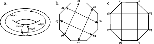
Our three-regular graphs describe a glueing of the -gon’s edges. If the toothpick portion of the three-regular graph contains an edge connecting vertex and vertex , then edge and edge are glued together in the corresponding -gon. This glueing maps the -gon to a graph embedded in a Riemann surface of genus . Since the complement of this graph is homeomorphic to the unit disc, we say the map has “one face”. Figure 1 shows a one-face map, its representation by a -gon with edge identifications, and the associated three-regular graph. All one-face maps can be represented by a three-regular graph of the form .
2 Numerical studies of one-face maps


We generated large samples of random matrices having the form , using Matlab’s random permutation generator. The limiting eigenvalue statistics of our random matrices are the same as those of much larger, and more widely studied classes. In particular, the limiting eigenvalue density is described by the McKay density [1], and the distribution of scaled eigenvalue spacings11 1 Spacings are found by ordering the eigenvalues in ascending order and finding the distance between consecutive eigenvalues. These distances are then scaled to have mean one and integrated density one. from the bulk of the spectrum appears to be that of the Gaussian Orthogonal Ensemble (GOE). Figure 2 shows the empirical eigenvalue density for a random sample of matrices. Figure 3 shows the scaled eigenvalue spacing distribution over the bulk of the spectrum for the same sample.
The McKay density formula,
| (1) |
describes the limiting eigenvalue density for sequences of of -regular graphs which look like trees at most vertices.
Theorem 2.1 (McKay).
Given a sequence of -regular graphs for some , let denote the number of vertices in graph , and the number of closed walks of length . If as , and
| (2) |
then the limiting probability density function describing the eigenvalues of is .
McKay proved that for a deterministic sequence of -regular graphs, if the limiting eigenvalue density is not described by McKay’s density formula, then the ratio of the number of closed walks of length to the number of vertices must not approach zero, for some value of .
The Gaussian Orthogonal Ensemble is the set of matrices whose components are independent (up to the symmetry requirement) random variables of mean zero and standard deviation one. Numerical studies have revealed that the distributions describing the eigenvalue statistics of the Gaussian Orthogonal Ensemble (GOE), describe the eigenvalue statistics of most real symmetric random matrices having independent entries. However, the entries of our random matrices are highly dependent. Since these matrices represent three-regular graphs, the entries of each row and each column must sum to three. Furthermore, the cycle subgraph ensures that two of the non-zero entries of each row and each column come from the first sub/super-diagonals of the matrix.
Given our random matrices describe one-face maps, a natural question is whether the eigenvalue statistics depend on the genus of the underlying map. To investigate this question we must generate matrices corresponding to random one-face maps having edges and genus .
3 Constructing genus zero maps
The number of genus one-face maps having edges in the embedded graph is given by [2, Theorem 2]
| (3) |
The vast majority of one-face maps having edges are of genus slightly less than . For a given , random selections of one-face maps will only sample genera near this upper bound. For large , the distribution of genera makes it infeasible to generate a random sample of low genus (relative to ) by generating random one-face maps and sorting out the maps with desired genus. We need an algorithm which will generate random one-face maps of a specified genus. In the genus zero case, the bijection between one-face maps and pair partitions provides such an algorithm.
As previously described, the important feature in the representation of one-face maps by three-regular graphs of the form is the toothpick subgraph, . This portion of the graph defines the edge glueings of the polygonal representation. This information can be encoded in a pair partition diagram. If vertex and vertex are adjacent in the toothpick subgraph, then node and node are paired in the associated pair partition. There is a bijection between the set of non-crossing pair partitions and genus zero one-face maps. Using this bijection, we have developed an algorithm to generate the adjacency matrices of three-regular graphs representing random genus zero one-face maps. The generation of one-face maps having specified genus and edges remains an open problem.

Our algorithm generates a random non-crossing pair partition and then uses the node identifications of this pair partition to assign adjacencies in the toothpick subgraph of the associated three-regular graph. Non-crossing pair partitions are formed recursively. The node paired with node one is randomly chosen according to the probability mass function described below. This pairing partitions the remaining nodes into two sets, one within the pairing and one external to it. The first node of each of these sets is then paired using the same algorithm. This process is repeated until all nodes have been paired.
The number of non-crossing pair partition on nodes is given by the Catalan number,
which can be defined recursively as
| (4) |
Let be the random variable representing the node paired with node one in a non-crossing pair partition. Since the pair partition is non-crossing, odd nodes must be paired with even nodes. The number of non-crossing pair partitions on nodes in which the first node is paired with node is equal to the number of non-crossing pair partitions on elements times the number of non-crossing pair partitions on elements, . Thus, the probability mass function () of is a function of both and , and is given by
| (5) |
To avoid computer arithmetic errors, the for greater than five and less than is calculated using the recursive formula derived from equation (4).
| (6) |
Our algorithm was implemented using Matlab. With each recursive call to our program, we assign a pairing to the first element of some subset of the entire pair partition. These subsets are determined by the previously assigned pairs. For the example shown in Figure 5, after the first pairing is assigned, the partition is divided into two subsets of lengths and . The first element of each of these subsets is paired during the next round of calls. Since the used to assign these pairings is based on the subset lengths, it is different for each recursive call.

3.1 Proof that genus zero one-face maps are chosen with equal probability
As previously discussed, randomly choosing a genus zero one-face map having edges is equivalent to randomly choosing a non-crossing pair partition on nodes. The number of non-crossing pair partitions on nodes is . Thus, we want our algorithm to construct non-crossing pair partitions on nodes in such a way that every partition has a chance of being created.
Induction Case: There is only one way to partition 2 nodes. Node 1 is paired with node 2 with probability 1, and the resulting non-crossing pair partition is chosen with probability .
Suppose that for all less than , the algorithm randomly constructs non-crossing pair partitions on nodes in such a way that each possible partition has the equal probability of being created, . Let be an arbitrary non-crossing pair partition of elements, and let node be the element paired with node one in . The probability our algorithm constructs partition is equal to the probability of node 1 being paired to node , times the probability of the particular non-crossing pair partition on the nodes internal to the pairing 1:, times the probability of the particular non-crossing pair partition on the nodes external to the pairing 1:. By our supposition, our algorithm creates the internal pair partition with probability , and the external pair partition with probability . Thus, the probability of an arbitrary non-crossing pair partition being created is equal to
| (7) | |||||
By induction, our algorithm randomly constructs non-crossing pair partitions on nodes with equal probability .
4 Results
We can examine the eigenvalue statistics of one-face maps having specified genus near by forming large samples of random one-face maps having edges and sorting by genus. Figures 6 and 7 show the eigenvalue density and spacing distribution for a random sample of genus 147 one-face maps generated in this way. Examining the eigenvalue statistics of one-face maps having genus near , we find that for large the eigenvalue density appears to be McKay, and the scaled spacing density appears to be that of the Gaussian Orthogonal Ensemble. These results are unsurprising given that samples of random one-face maps for large exhibit the same properties and are comprised primarily of maps having genera near .


Using the previously described algorithm, we generated samples of random genus zero one-face maps for large , and examined the eigenvalue statistics. The results are strikingly different from those found for one-face maps having genus near . The distribution of eigenvalues for a random sample of genus zero one-face maps is plotted in Figure 6. In Figure 8 the eigenvalue density curves for various samples of genus zero one-face maps are plotted on the same axis. Although the number of embedded edges is different for each sample, the eigenvalue densities are nearly identical. While this distribution is the same for all large values of , it does not appear to be described by any established density formula. Examining the eigenvalues themselves, we find that the peaks observed in the density curve near and are not the result of repeated eigenvalues, but rather a decrease in spacing between consecutive eigenvalues. The non-crossing structure of the toothpick portion of the three-regular graphical representation of genus zero one-face maps ensures that the graphs are bipartite. The symmetry in the distribution of eigenvalues about is due to this bipartite structure.

The difference in the distribution of eigenvalues for the genus zero and genus cases is also seen in the corresponding mean spacing curves. Figure 9 shows the mean eigenvalue spacing as a function of for a sample of three-regular graphs representing genus zero one-face maps, and a sample of three-regular graphs representing one-face maps of genera near .

It is clear from these results that, in the genus zero case, the distribution of eigenvalues is not described by the McKay density formula. In fact, three-regular graphs representing genus zero one face maps violate the criteria of McKay’s theorem (2.1). These graphs are always planar, i.e. they can be drawn in the plane in such a way that the edges of the graph do not intersect except at vertex points. A planar drawing of a graph divides the set of points of the plane not lying on the graph into regions called faces. Figure 10 shows the three-regular graph representing a genus zero one-face map with its faces labeled. One of the faces will be unbounded. This face is called the infinite face. All other faces are bounded by the edges of the graph, and are called internal faces.

For genus zero one-face maps, the embedded graph is a planar tree, and each internal face of the associated three-regular graph corresponds to a vertex of this embedded tree. The degree of this embedded vertex is equal to the face boundary length. Thus, the distribution of vertex degrees in the genus zero embedded trees determines the distribution of face boundary lengths in the associated three-regular graph. Furthermore, since each face boundary forms a cycle in the graph, the number of vertices of degree in the tree provides a lower bound for the number of cycles in the three-regular graph.
Let denote the set of three-regular graphs having vertices which represent genus zero one-face maps. Drmota and Gittenberger [3] proved that the number of degree vertices in a random planar tree having edges is asymptotically . Thus, the expected number of -cycles in a random element of as is
Since the number of closed walks of length is greater than or equal to the number of cycles of length , the set of three-regular graphs representing genus zero one-face maps contains a subset of nonzero measure for which
This violates the criteria of McKay’s Theorem.
The distribution of scaled eigenvalue spacings for a sample of random genus zero one-face maps having edges is plotted in Figure 7. The scaled spacings in the genus zero case are not described by the GOE density formula which was shown numerically to describe the bulk scaling limit for genera near , but rather appear to be described by the exponential probability density function.
5 Conclusion and conjecture
The numerical results suggest that the eigenvalue statistics depend on the rigidity of the associated three-regular graph. For one-face maps having small genus relative to , a great deal of structure is imposed on the corresponding three-regular graph. We believe the striking difference between the eigenvalue statistics of genus zero maps and genus is a result of this imposed structure. For any fixed genus, as the size of the map increases (i.e. the number of vertices in the associated three-regular graph grows), more structure will be imposed on the associated three-regular graph. This leads to the conjecture that for fixed genus , in the limit as , the scaled spacing distribution will be exponential. As we have seen, for , the scaled spacing distribution appears to be GOE. Thus the distribution must undergo a shift from GOE to exponential as increases. Similar shifts in probability density functions have been observed in biological networks and quantum chaotic systems [4, 5].
References
- [1] B. McKay, The expected eigenvalue distribution of a large regular graph, Linear Algebra and its Applications, 40(1981), 203-216.
- [2] J. Harer and D. Zagier, The Euler characteristic of the moduli space of curves, Inventiones Mathematicae, 85(3)(1986), 457-485.
- [3] M. Drmota and B. Gittenberger, The distribution of nodes of given degree in random trees, Journal of Graph Theory, 31(3)(1999), 227-253
- [4] E. B. Bogomolny, B. Georgeot, M. Giannoni, and C. Schmit, Arithmetical chaos. Physics Reports, 291(1997), 219-324
- [5] F. Luo, J. Zhong, Y. Yang, R. Scheuermann, and J. Zhou, Application of random matrix theory to biological networks, arXiv:q-bio/0503035v1