Classical phases and quantum angles in the description of interfering Bose-Einstein condensates

W. J. Mullin^a and F. Laloë^b Affiliation: ^aDepartment of Physics, University of Massachusetts, Amherst, Massachusetts 01003 USA
^bLaboratoire Kastler Brossel, ENS, UPMC, CNRS; 24 rue Lhomond, 75005 Paris, France Email: mullin@physics.umass.edu;laloe@lkb.ens.fr

Abstract

The interference of two Bose-Einstein condensates, initially in Fock states, can be described in terms of their relative phase, treated as a random unknown variable. This phase can be understood, either as emerging from the measurements, or preexisting to them; in the latter case, the originating states could be phase states with unknown phases, so that an average over all their possible values is taken. Both points of view lead to a description of probabilities of results of experiments in terms of a phase angle, which plays the role of a classical variable. Nevertheless, in some situations, this description is not sufficient: another variable, which we call the “quantum angle”, emerges from the theory. This article studies various manifestations of the quantum angle. We first introduce the quantum angle by expressing two Fock states crossing a beam splitter in terms of phase states, and relate the quantum angle to off-diagonal matrix elements in the phase representation. Then we consider an experiment with two beam splitters, where two experimenters make dichotomic measurements with two interferometers and detectors that are far apart; the results lead to violations of the Bell-Clauser-Horne-Shimony-Holt inequality (valid for local-realistic theories, including classical descriptions of the phase). Finally, we discuss an experiment where particles from each of two sources are either deviated via a beam splitter to a side collector or proceed to the point of interference. For a given interference result, we find “population oscillations” in the distributions of the deviated particles, which are entirely controlled by the quantum angle. Various versions of population oscillation experiments are discussed, with two or three independent condensates.

I Introduction

If two or more Bose-Einstein condensates (BEC) merge, they produce a density interference pattern, as shown by spectacular experiments with alkali atoms [1]. The usual explanation is that, when spontaneous symmetry breaking (SSB) takes place at the Bose-Einstein transition, each condensate acquires a random but well-defined phase. The interference pattern then exhibits the relative phase. The simplest form of this view involves the use of a classical complex variable for each condensate given by

\left\langle\psi_{\alpha,\beta}(\mathbf{r})\right\rangle=\sqrt{n_{\alpha,\beta}(\mathbf{r})}e^{i\phi_{\alpha,\beta}(\mathbf{r)}}

(1)

where $n_{\alpha,\beta}(\mathbf{r)}$ are the condensate densities and $\phi_{\alpha,\beta}(\mathbf{r)}$ their phases. Another quantum treatment of the problem can be carried out by the use of “phase states,” which describe a state of two condensates having a known relative phase and a fixed total number of particles [2] - we will discuss the use of phase states in the next section. For systems containing many particles the phase then appears as a macroscopic quantity that has classical properties, but takes completely independent random values from one realization of the experiment to the next.

However, Bose-Einstein condensates are naturally described by Fock states, states of definite particle number, for which the phase is completely undetermined. Various authors [3, 4, 5, 6, 7, 8, 9, 10] have shown that repeated quantum measurements of the relative phase of two Fock states cause a well-defined value to emerge spontaneously, but with a random value. The probability of finding $M$ particles, out of a total of $N$ , at positions $\mathbf{r}_{1},\cdots\mathbf{r}_{M}$ ( $M\ll N$ ) is shown to be given by

P(\mathbf{r}_{1},\cdots\mathbf{r}_{M})\sim\int_{-\pi}^{\pi}\frac{d\lambda}{2\pi}\prod_{i=1}^{M}\left[1+\cos(\mathbf{k}\cdot\mathbf{r}_{i}+\lambda)\right]

(2)

where $\mathbf{k}$ is the wave number difference between the two condensates. The product in the integrand can be interpreted as describing the independent individual measurements of position with the interference of two waves of relative phase $\lambda$ , resulting in probability $\left[(1+\cos(\mathbf{k}\cdot\mathbf{r}_{i}+\lambda)\right]/2$ ; the $\lambda$ integration expresses that this phase is initially completely unknown. Nevertheless, after a series of measurements has been performed (still for $M\ll N$ ), the product of these probabilities in Eq. (2) is found to peak sharply at some particular value $\lambda_{0},$ which becomes better and better defined while the experiments accumulate, but takes a completely uncorrelated random value from experiment to experiment. Fig. 1 illustrates the peaking effect in the integrand in Eq. (2) after 200 measurements (the method by which we choose the position values is given in Ref. [11]).

Refer to caption — Figure 1: The integrand $\prod_{i=1}^{M}\left(1+\cos(\mathbf{k}\cdot\mathbf{r}_{i}+\lambda)\right)$ of Eq. (2) as a function $\lambda$ after 200 measurements at positions $\mathbf{r_{\mathit{\mathit{i}}}}.$ These first 200 measurements essentially convert a double Fock state into a state resembling a phase state, peaked sharply at some particular value $\lambda_{0},$ , which is completely random from experiment to experiment.

Eq. (2) is quite capable of describing the interference pattern seen in the MIT experiment [11]. Note however that the average over all possible phases makes the phase very similar to the integrated variable $\lambda$ in Bell’s theorem [12], or to an “element of reality” as defined by Einstein, Podolsky and Rosen [13] - and we know that this notion combined with locality leads to contradictions with quantum mechanics. Eq. (2) can thus be seen as a “classical” equation, which is unlikely to be able to describe some truly quantum experiments (for instance, it cannot violate Bell’s theorem).

In some conditions, quantum interference effects arise so that the description in terms of a classical phase is no longer sufficient; a second angle (or its equivalent) becomes necessary: the “quantum angle,” which controls the amount of “quantumness” in the results of an interference experiment. This article discusses the role of the quantum angle in general. While it is possible to carry out such a discussion for the position measurements in free space, as in Eq. (2), it turns out that interferometers with dichotomic outputs provide especially interesting results, for instance in terms of quantum non-locality; this is why interferometers will be the central subject of this paper.

In Sec. II we show how this quantum angle already appears in a very simple situation, with one single beam splitter on which two Fock states interfere; we relate the quantum angle to phase off-diagonal terms. In Sec. III we study the effects of the quantum angle in an experiment with an interferometer providing dicthotomic results in two different regions of space, and leading to violations of the Bell inequalities. But other experiments involving directly the quantum angle are also possible. One was suggested to us by the recent article of Dunningham et al [16], who considered the interference pattern of three merging condensates and the resulting “phase Schrödinger cat state” formed by the remaining (non-measured) particles. In Sec. IV we consider a simplified version of this experiment with two condensates only, which interfere on a beam splitter; among the total of $N$ particles, only $M$ interfere and are detected at locations 1 and 2; the remaining are deflected near their sources and separately counted in detectors 3 and 4 ( $m_{\alpha}$ particles from condensate $\alpha$ , and $m_{\beta}$ particles from condensate $\beta$ ). For fixed numbers of such particles in detectors 1 and 2, the numbers found in detectors 3 and 4, as a function of $m_{\alpha}$ , are found to have an oscillating distribution - a “fringe” pattern when plotted over an ensemble of such experiments. We will see that this effect, which we call “population oscillations” (PO), involves the interference of two peaks in the quantum angle distribution; thus such an experiment would also directly reveal the existence of the quantum angle. One can show [17] how these oscillations represent an example of quantum interference of macroscopically distinct states (QiMDS), a property of quantum mechanics that can verify its validity in large scale systems [18].

II A simple interferometer

In the derivation of [10, 14, 15], both the classical phase $\lambda$ and the quantum angle $\Lambda$ had similar origins: conservation rules, which take the form of integrals over these angles. Here we show that phase states can also be used to obtain the same results, following a reasoning that is similar to that found, for instance, in Ref. [2]. Mathematically, of course, the two derivations are equivalent; but, physically, it is interesting to obtain the same results from two different points of view.

We consider the experiment schematized in Fig. 2, where two Fock states with populations $N_{\alpha}$ , and $N_{\beta}$ are emitted by two sources, cross a beam splitter, and interfere in the regions of detection 1 and 2. Despite the apparent simplicity of this device we have shown in a recent paper that remarkably complex detector distributions can result [19]. The double Fock state describing the sources is

\left|N_{\alpha},N_{\beta}\right\rangle=\frac{1}{\sqrt{N_{\alpha}!N_{\beta}!}}a_{\alpha}^{\dagger N_{\alpha}}a_{\beta}^{\dagger N_{\beta}}\left|\text{0}\right\rangle

(3)

where $\left|\text{0}\right\rangle$ is the vacuum state and $a_{\alpha}^{\dagger}$ creates particle in state $\alpha$ corresponding to one source and $a_{\beta}^{\dagger}$ creates a $\beta$ -state particle corresponding to the other source. The total number of particles is $N=N_{\alpha}+N_{\beta}$ .

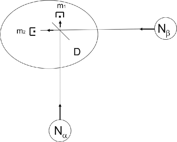
The destruction operators $a_{1}$ and $a_{2}$ associated with the output modes can be written in terms of the mode operators at the sources $a_{\alpha},$ $a_{\beta}$ by tracing back from the detectors to the sources, with a phase shift of $\pi/2$ at each reflection:

a_{1}=\frac{1}{\sqrt{2}}\left[a+ia_{\beta}\right]\;;\;a_{2}=\frac{1}{\sqrt{2}}\left[ia_{\alpha}+a_{\beta}\right]

(4)

The probability amplitude describing the system after crossing the beam splitter with $m_{1},m_{2}$ particles in the detector regions is

C_{m_{1},m_{2}}=\left\langle 0\left|\frac{a_{1}^{m_{1}}a_{2}^{m_{2}}}{\sqrt{m_{1}!m_{2}!}}\right|N_{\alpha},N_{\beta}\right\rangle

(5)

with $m_{1}+m_{2}=N$ . To compute the state $a_{1}^{m_{1}}a_{2}^{m_{2}}\left|N_{\alpha},N_{\beta}\right\rangle$ , we expand the double Fock state in normalized (relative) phase states, defined for two condensates (with constant total particle number $N$ ) as

	$\displaystyle\left\|\phi,N\right\rangle$	$\displaystyle=$	$\displaystyle\frac{1}{\sqrt{2^{N}N!}}(a_{\alpha}^{\dagger}+e^{i\phi}a_{\beta}^{\dagger})^{N}\left\|0\right\rangle=$		(6)
		$\displaystyle=$	$\displaystyle\frac{1}{\sqrt{2^{N}N!}}\sum_{n=0}^{N}\frac{N!}{\sqrt{n!(N-n)!}}\;e^{i\phi(N-n)}\left\|n,N-n\right\rangle$		(6)

where $N=N_{\alpha}+N_{\beta}$ . The expansion in terms of the phase states is

\left|N_{\alpha}N_{\beta}\right\rangle=\sqrt{\frac{2^{N}N_{\alpha}!N_{\beta}!}{N!}}\int_{-\pi}^{\pi}\frac{d\phi}{2\pi}e^{-iN_{\beta}\phi}\left|\phi,N\right\rangle

(7)

The action on phase states of the operators $a_{i}$ given in (4) is particularly simple; if we write them as

a_{i}=v_{i\alpha}a_{i\alpha}+v_{i\beta}a_{\beta},

(8)

(with $v_{i\alpha}$ and $v_{i\beta}$ identified by Eqs. (4)) we merely obtain¹¹ 1 The phase state is obtained by repeated actions of the creation operator $a_{\phi}^{\dagger}=(a_{\alpha}^{\dagger}+e^{i\phi}a_{\beta}^{\dagger})$ over vacuum, but no action of the “orthogonal” creation operator $a_{\phi+\pi/2}^{\dagger}$ ; the action of the annihilation operator associated to the former operator is therefore simple, while that of the latter gives zero. Expanding the $a_{i}$ ’s over the $a_{\alpha,\beta}$ , and then over $a_{\phi}$ and $a_{\phi+\pi/2}$ , and keeping only the component on the first annihilation operator, then directly leads to (9). [11]:

a_{i}\left|\phi,N\right\rangle=\sqrt{\frac{N}{2}}(v_{i\alpha}+v_{i\beta}e^{i\phi})\left|\phi,N-1\right\rangle

(9)

Applying this result several times to (7) then gives

a_{1}^{m_{1}}a_{2}^{m_{2}}\left|N_{\alpha}N_{\beta}\right\rangle=\sqrt{\frac{N_{\alpha}!N_{\beta}!}{2^{N}}}\int_{-\pi}^{\pi}\frac{d\phi}{2\pi}R(\phi)\left|\,0\right\rangle

(10)

where $m_{1}+m_{2}=N$ and

R(\phi)=2^{N/2}e^{-iN_{\beta}\phi}(v_{1\alpha}+v_{1\beta}e^{i\phi})^{m_{1}}(v_{2\alpha}+v_{2\beta}e^{i\phi})^{m_{2}}=e^{-iN_{\beta}\phi}(1+ie^{i\phi})^{m_{1}}(i+e^{i\phi})^{m_{2}}

(11)

When we insert this result into Eq. (5) and take the square modulus, we obtain the probability in the form:

P_{m_{1}m_{2}}=\frac{N_{\alpha}!N_{\beta}!}{m_{1}!m_{2}!}\int_{-\pi}^{\pi}\frac{d\phi^{\prime}}{2\pi}\int_{-\pi}^{\pi}\frac{d\phi}{2\pi}R^{*}(\phi^{\prime})R(\phi)

(12)

and find upon multiplying all these factors out:

	$\displaystyle P_{m_{1}m_{2}}$	$\displaystyle=$	$\displaystyle\frac{N_{\alpha}!N_{\beta}!}{m_{1}!m_{2}!}\int_{-\pi}^{\pi}\frac{d\phi^{\prime}}{2\pi}\int_{-\pi}^{\pi}\frac{d\phi}{2\pi}\cos[(N_{\alpha}-N_{\beta})\left(\phi-\phi^{\prime}\right)/2]$		(13)
			$\displaystyle\times\left[\cos\left(\frac{\phi-\phi^{\prime}}{2}\right)+\cos\left(\frac{\phi+\phi^{\prime}-\pi}{2}\right)\right]^{m_{1}}\left[\cos\left(\frac{\phi-\phi^{\prime}}{2}\right)-\cos\left(\frac{\phi+\phi^{\prime}-\pi}{2}\right)\right]^{m_{2}}$		(13)

It is then natural to make a variable change by introducing the average of the two phases

\lambda=(\phi+\phi^{\prime}-\pi)/2

(14)

now identified as “the phase angle”, as well as the difference

\Lambda=(\phi-\phi^{\prime})/2

(15)

which we call the “quantum angle.” Eq. (13) then becomes

	$\displaystyle P_{m_{1}m_{2}}$	$\displaystyle=$	$\displaystyle\frac{N_{\alpha}!N_{\beta}!}{N!}\frac{1}{m_{1}!m_{2}!}\int_{-\pi}^{\pi}\frac{d\Lambda}{2\pi}\int_{-\pi}^{\pi}\frac{d\lambda}{2\pi}\cos[(N_{\alpha}-N_{\beta})\Lambda]$		(16)
			$\displaystyle\times\left[\cos\left(\Lambda\right)+\cos\left(\lambda\right)\right]^{m_{1}}\left[\cos\left(\Lambda\right)-\cos\left(\lambda\right)\right]^{m_{2}}$		(16)

This probability is a double sum over the variables $\lambda$ and $\Lambda$ of a function of these variables as well as of the results $m_{1}$ and $m_{2}$ . According to (15), if one sets $\Lambda=0$ or $\Lambda=\pm\pi$ in this function, one obtains the contributions of the terms that are diagonal in the phase representation. The relevant values of the phase in the initial state then appear directly. For instance, if the function has a single narrow peak around some particular value, the phase is well-defined; if it has several peaks at various values of the phase, for a pure state the system is in a coherent superposition of different values of the phase (a “Schrödinger cat” if these values are very different and if the system contains many particles). The role of the quantum angle $\Lambda$ is precisely to signal the coherent character of the different values of the phase (off-diagonal terms in the phase representation). Each time non-zero values of this quantum angle play a role, the classical description of Eq. (2) is not sufficient; the non-classical behavior occurs because the factors $\left[\cos\left(\Lambda\right)\pm\cos\left(\lambda\right)\right]/2$ in the integrand of (16) can become negative, so that they can no longer be interpreted as probabilities. In the ( $\lambda$ , $\Lambda$ ) plane, we will call the “classical region” the region that lies around the $\lambda$ axis at $\Lambda=0$ , and the ‘‘quantum region’’ the rest of the plane.²² 2 The regions at $\Lambda=\pm\pi$ are also classical (i.e., equivalent to $\Lambda=0$ ), as can be seen by showing that the integration segments $-\pi\leq\Lambda\leq-\pi/2$ and $\pi/2\leq\Lambda\leq\pi$ (or equivalently $\pi/2\leq\Lambda\leq 3\pi/2$ ) give an identical contribution as the region $-\pi/2\leq\Lambda\leq\pi/2$ . To do so make the substitution $\Lambda^{\prime}=\Lambda-\pi$ and $\lambda^{\prime}=\lambda-\pi$ .

In Fig. 3(a), we see the absolute square of the coefficient $R$ of Eq. (11), showing two peaks for a particular choice of $m_{1}$ and $m_{2}$ and with $N_{\alpha}=N_{\beta}$ and $M=N$ . This is not surprising since, classically, an ambiguity in the sign of the phase angle difference also occurs in this interferometer: two different values of this difference lead to the same intensities in the two output arms. Fig. 3(b) shows a plot of the corresponding integrand of Eq. (16). The diagonal phase contributions arise from the peaks on the lines $\Lambda=0,\pm\pi$ . Here the system is in a pure state, so that these peaks are necessarily coherent; peaks in the quantum regions (away from $\Lambda=0,\pm\pi.$ ) are also visible, which have a negative sign and therefore signal destructive interference (for these particular results of measurement; for other values, it is constructive).

In Fig. 4 we show a particular example of the probability distribution for finding the set of $\{m_{1},m_{2}\}$ particles in the detectors. The structure has a surprisingly complex dependence on the numbers of particles in the Fock state inputs. The simple interferometer is discussed more completely in a separate publication [19].

In this section we have recovered by the use of phase states the basic results obtained from conservation rules in [10, 14]. The present method illustrates the relation between the two angles and the diagonal or off-diagonal phase terms, and therefore the role of the classical and non-classical region in the $\lambda$ , $\Lambda$ plane. We now examine how the quantum angle changes the description of some other processes for Bose-Einstein condensates involving several interferometers.

III Double interferometer

We now discuss the role of the quantum angle in an interferometer experiment designed to observe violations of the Bell-Clauser-Horne-Shimony-Holt (BCHSH) inequality [20], already discussed in [14]. The device is shown in Fig. 5 and involves a twin Fock state entering a double interferometer, which can be used to measure the relative phase of the two condensates in two remote regions of space. The relevance of twin Fock states for phase measurements in simple interferometers was already discussed in Ref. [21] in 1993. The measurement of the phase of an arbitrary quantum state at different locations of space was discussed in Ref. [22] in 1994. A general discussion of the properties of the quantum operator associated with the phase difference between two modes can be found in Ref. [23]. A more recent Ref. [24] gives a discussion of the interference of two Fock states and of the details of the statistics of the position measurements, in the context of interferences in free space.

III.1 Quantum calculation

For completeness, we briefly recall the quantum calculation in this subsection. The destruction operators $a_{1}\cdots a_{4}$ associated with the output modes can be written in terms of the mode operators at the sources $a_{\alpha},a_{\beta},a_{\alpha^{\prime}}$ and $a_{\beta^{\prime}}$ by tracing back from the detectors to the sources, with a phase shift of $\pi/2$ at each reflection, $\zeta$ or $\theta$ at the shifters, and a $1/\sqrt{2}$ at each beam splitter. This gives the projections of the two different source modes onto each detector mode

	$\displaystyle a_{1}$	$\displaystyle=$	$\displaystyle\frac{1}{2}\left[ie^{i\zeta}a_{\alpha}+ia_{\beta}\right];\qquad a_{2}=\frac{1}{2}\left[-e^{i\zeta}a_{\alpha}+a_{\beta}\right]$
	$\displaystyle a_{3}$	$\displaystyle=$	$\displaystyle\frac{1}{2}\left[ia_{\alpha}+ie^{i\theta}a_{\beta}\right];\qquad a_{4}=\frac{1}{2}\left[a_{\alpha}-e^{i\theta}a_{\beta}\right]$		(17)

where we have eliminated $a_{\alpha^{\prime}}$ and $a_{\beta^{\prime}}$ , which contribute only vacuum. The source state, having $N_{\alpha}$ and $N_{\beta}$ particles in the two condensates is again given by Eq. (3). The amplitude describing the system crossing all beam splitters with $m_{1}\cdots m_{4}$ particles in the detectors is

C_{m_{1},..,m_{4}}=\left\langle m_{1},m_{2},m_{3},m_{4}\right|\Phi\rangle~=\left\langle 0\right|\frac{a_{1}^{m_{1}}\cdots a_{4}^{m_{4}}}{\sqrt{m_{1}!\cdots m_{4}!}}\frac{a_{\alpha}^{\dagger N_{\alpha}}a_{\beta}^{\dagger N_{\beta}}}{\sqrt{N_{\alpha}!N_{\beta}!}}\left|0\right\rangle

(18)

The calculation is similar to that of Sec. II and can be found in Refs. [14, 15]. We substitute (17) into this expression, make binomial expansions of the sums, evaluate the expectation value of the operators, replace Kronecker $\delta$ ’s by integrals in the form $\delta_{N_{\gamma},p}=\int_{-\pi}^{\pi}\frac{d\lambda_{\gamma}}{2\pi}~e^{i(p-N_{\gamma})\lambda_{\gamma}}$ with $\gamma=\alpha,\beta$ , and make an appropriate variable change. We then obtain

\mathcal{P}(m_{1},m_{2},m_{3},m_{4})=\frac{2^{-N}\,N_{\alpha}!N_{\beta}!}{m_{1}!\cdots m_{4}!}\int_{-\pi}^{\pi}\frac{d\lambda}{2\pi}\int_{-\pi}^{\pi}\frac{d\Lambda}{2\pi}\cos[(N_{\alpha}-N_{\beta})\Lambda]\prod_{i=1}^{4}\left[\cos\Lambda+\eta_{i}\cos\left(\lambda-\varphi_{i}\right)\right]^{m_{i}}

(19)

where $\eta_{1}=\eta_{3}=1$ ; $\eta_{2}=\eta_{4}=-1$ ; $\varphi_{1}=\varphi_{2}=-\zeta$ ; $\varphi_{3}=\varphi_{4}=\theta$ . In [15] we also consider the case where only $M$ particles are measured among a total number of $N$ , by assuming losses of particles either near the sources or near the detectors. The sum of the probabilities associated with the orthogonal states corresponding to the result of measurement is then

\mathcal{P}(m_{1},m_{2},m_{3},m_{4})=\frac{2^{N-2M}M!(N/2!)^{2}}{N!\,m_{1}!\cdots m_{4}!}\int_{-\pi}^{\pi}\frac{d\lambda}{2\pi}\int_{-\pi}^{\pi}\frac{d\Lambda}{2\pi}[\cos\Lambda]^{N-M}\prod_{i=1}^{4}\left[\cos\Lambda+\eta_{i}\cos\left(\lambda-\varphi_{i}\right)\right]^{m_{i}}

(20)

(for simplicity, from now on we assume that $N_{\alpha}=N_{\beta}$ ; the probabilities have now been normalized to a total probability of $1$ for all events associated with the detection of $M$ particles).

We have associated values of $\eta$ that are +1 for channels of detection 1 and 3, $-1$ for channels detectors 2 and 4. Assume now that Alice, in the first detection region 1, calculates the product of all $\eta$ values that she obtains, that is the local parity $(-1)^{m_{2}}$ , which is called $\mathcal{A}=\pm 1$ ; similarly Bob, in the second detection region 2, calculates $\mathcal{B}=(-1)^{m_{4}}=\pm 1$ . We then have two functions to which the BCHSH theorem can be applied. The quantum average of their product is:

\left\langle\mathcal{AB}\right\rangle=\sum_{m_{1}\cdots m_{4}}(-1)^{m_{2}+m_{4}}\mathcal{P}(m_{1},m_{2},m_{3},m_{4})

(21)

The result for the case where all particles are measured ( $M=N)$ is found to be [14]:

\left\langle\mathcal{AB}\right\rangle=\left[\cos\left(\frac{\zeta+\theta}{2}\right)\right]^{N}

(22)

III.2 Classical phase situations

We consider the case where $M\ll N$ particles are detected; in (20), the factor $\left[\cos\Lambda\right]^{N-M}$ is peaked sharply at $\Lambda=0$ . Setting $\cos\Lambda$ to unity in the product and doing the integral over $\Lambda$ gives

\mathcal{P}(m_{1},m_{2},m_{3},m_{4})=\frac{M!}{4^{M}m_{1}!\cdots m_{4}!}\int_{-\pi}^{\pi}\frac{d\lambda}{2\pi}\prod_{i=1}^{4}\left[1+\eta_{i}\cos\left(\lambda-\varphi_{i}\right)\right]^{m_{i}}

(23)

where we have taken the $N\rightarrow\infty$ limit of the normalization factor. The quantum angle $\Lambda$ has now disappeared from the result, so that in the integrand all the terms in the product are positive and can be interpreted as probabilities. The BCHSH inequality [20] then provides

\left\langle\mathcal{AB}\right\rangle+\left\langle\mathcal{AB}^{\prime}\right\rangle+\left\langle\mathcal{A}^{\prime}\mathcal{B}\right\rangle-\left\langle\mathcal{A}^{\prime}\mathcal{B}^{\prime}\right\rangle\leq 2

(24)

where letters with and without primes imply measurements at differing angles. No violation of this inequality is possible as long as (23) applies.

This inequality can also be checked explicitly by computing the value of the average $\left\langle\mathcal{AB}\right\rangle$ from (23); we find

\left\langle\mathcal{AB}\right\rangle=\frac{M!}{(\frac{M}{2}!)^{2}2^{M}}\left[\cos\left(\frac{\zeta+\theta}{2}\right)\right]^{M}

(25)

III.3 Fully quantum situations

We now assume that all particles are measured. For convenience, Alice’s measurement angle is taken as $\phi_{a}=\zeta/2$ and Bob’s as $\phi_{b}=-\theta/2$ . We define $E(\phi_{a}-\phi_{b})=\cos^{N}\left(\phi_{a}-\phi_{b}\right)$ , set $\phi_{a}-\phi_{b}=\phi_{b}-\phi_{a^{\prime}}=\phi_{b^{\prime}}-\phi_{a}=\xi$ and $\phi_{b^{\prime}}-\phi_{a^{\prime}}=3\xi$ . We now maximize $Q=3E(\xi)-E(3\xi)$ in order to find the greatest violation of the inequality for each $N$ . For $N=2$ we find $Q_{\max}=2.41$ at $\xi=0.39$ ; for $N=4,$ $Q_{\max}=2.36$ at $\xi=0.26$ ; and for $N\rightarrow\infty,$ $Q_{\max}\rightarrow 2.32$ with $\xi\cong 0.52/\sqrt{N}$ . The system continues to violate local realism for arbitrarily large condensates.

Despite the identical dependence in the cosine factor in (25) and (22), the effect of the prefactor, always equal to or less than 1/2 in the classical case, is to prevent the violations of the inequalities to occur. Actually, quantum violations disappear even when only one particle is missed in the measurement process ( $M=N-1$ ) as discussed in Ref. [14].

III.4 Discussion

It is interesting to see in more detail how the quantum angle is involved in the BCHSH violation. For instance, Fig. 6 shows the variations as a function of $\lambda$ and $\Lambda$ of the function that appears in the integral of Eq. (20), for $N_{\alpha}=N_{\beta}=M=40$ , and $\theta=\zeta=0$ . The left part of the figure assumes that $m_{1}=6$ , $m_{2}=14$ , $m_{3}=14$ and $m_{4}=6$ , the right part that $m_{1}=6$ , $m_{2}=14$ , $m_{3}=15$ and $m_{4}=5$ ; one immediately notices that, depending on the parity of the sum $m_{2}+m_{4}$ , the peaks in the “quantum region” $\Lambda\neq 0$ have the opposite sign. This explains why the quantum effects will be enhanced if Alice and Bob decide to choose the parities (product of all their results $\eta$ ’s) as their local observables $\mathcal{A}$ and $\mathcal{B}$ . It is then natural that strong violations of the BCHSH inequalities should be obtained for this particular choice, while of course Alice and Bob could combine their local results in many other ways to obtain functions $\mathcal{A}$ and $\mathcal{B}$ .

Suppose now we delete the leading normalization factors in each of Eqs. (20) and (23) and then evaluate the unnormalized values of $\left\langle\mathcal{AB}\right\rangle$ for $M=2.$ The result in each case is $4$ $\left[\cos\left(\frac{\zeta+\theta}{2}\right)\right]^{2}$ . Thus the entire difference between quantum and classical averages is in the normalization given, respectively, by the integrals over $\Lambda$ and $\lambda$ of

	$\displaystyle L_{qu}(\xi,\Lambda,\lambda)$	$\displaystyle=$	$\displaystyle\sum_{m_{1}\cdots m_{4}}^{\prime}\left[\cos\Lambda+\eta_{i}\cos\left(\lambda+\zeta\right)\right]^{m_{1}}\left[\cos\Lambda+\eta_{i}\cos\left(\lambda+\zeta\right)\right]^{m_{2}}$		(26)
			$\displaystyle\times\left[\cos\Lambda+\eta_{i}\cos\left(\lambda-\theta\right)\right]^{m_{3}}\left[\cos\Lambda+\eta_{i}\cos\left(\lambda-\theta\right)\right]^{m_{4}}$		(26)

where the sum is on all $m_{i}$ totaling 2; and

	$\displaystyle L_{cl}(\xi,\lambda)$	$\displaystyle=$	$\displaystyle\sum_{m_{1}\cdots m_{4}}^{\prime}\left[1+\eta_{i}\cos\left(\lambda+\zeta\right)\right]^{m_{1}}\left[1+\eta_{i}\cos\left(\lambda+\zeta\right)\right]^{m_{2}}$		(27)
			$\displaystyle\times\left[1+\eta_{i}\cos\left(\lambda-\theta\right)\right]^{m_{3}}\left[1+\eta_{i}\cos\left(\lambda-\theta\right)\right]^{m_{4}}$		(27)

For $M=2$ we explicitly get

	$\displaystyle L_{qu}(\xi,\Lambda,\lambda)$	$\displaystyle=$	$\displaystyle 8\cos^{2}\Lambda$		(28)
	$\displaystyle L_{cl}(\xi,\lambda)$	$\displaystyle=$	$\displaystyle 8$		(29)

The quantum normalization integrand clearly yields a smaller normalization integral enhancing the $\left\langle\mathcal{AB}\right\rangle$ average and allowing the violation of the BCHSH inequality. It is this variation with quantum angle that allows the violation.

IV Population oscillations

Dunningham et al [16] have considered a situation in which three condensates, a, b, and c, each contain initially $N/3$ particles. A number of them, $M<N$ , form an interference pattern on a screen, while the remaining particles $m_{a},m_{b,}$ and $m_{c}$ are counted elsewhere (perhaps having been deflected by beam splitters while traveling from the sources), or in a second step of the experiment. The numbers of such particles, as a function of $m_{a}$ and $m_{b}$ , are found to have an oscillating distribution when plotted over an ensemble of experiments corresponding to the same interference pattern for the first $M$ particles. This phenomenon was explained as arising from the interference of the two coherent components of a phase “Schrödinger cat state” of the system.

IV.1 Population oscillations by two-source interferometer

Here we present a simpler version of this experiment based on the interferometer shown in Fig. 7, which nevertheless retains the essential features of the three condensate device. The general idea is that condensates provide, in a sense, many realizations of the same single particle quantum state, since they contain many particles in the same individual state. One can then perform experiments where some particles are used to measure one quantum observable, some others another “incompatible” observable, which would be impossible with one single realization of the quantum state. In this case, the incompatible (non-commuting) observables will be the phase and the number of particles.

IV.1.1 Experimental setup

In our version of the experiment, $M$ particles from the two sources interfere in the detector D made up of a beam splitter and subdetectors 1 and 2; the other particles are detected before they reach the interferometer, with the help of additional beam splitters followed by detectors 3 and 4. For the sake of simplicity, we assume that all beam splitters have 1/2 reflectivity and transmissivity; we write $m_{1}$ and $m_{2}$ as the number of particles seen at subdetectors 1 and 2, respectively (with $M=m_{1}+m_{2}$ ), $m_{\alpha}$ and $m_{\beta}$ the number of particles seen in detectors 3 and 4. In this scheme, some of the particles are used to measure the relative phase of the two sources $N_{\alpha}$ and $N_{\beta}$ , the others to obtain information about their initial populations.

Assume for a moment that the central beam splitter is removed, so that no interference effect between the sources takes place at detectors 1 and 2. Then the experiment separates into two independent parts: the detectors 1 and 3 measure the population of one source, and the sum $m_{1}+m_{\alpha}$ gives an exact measurement of the initial population $N_{\alpha}$ ; of course $m_{1}$ and $m_{\alpha}$ may fluctuate separately, with a constant sum, but their most likely value is $N_{\alpha}/2$ . Similarly, detectors 2 and 4 give information on the population of the other source, and the most likely number of their counts is $N_{\beta}/2$ .

Now, when the central beam splitter is inserted, the counts of detectors 1 and 2 can no longer be ascribed to any of the sources, which are indistinguishable for the detectors; what they actually measure is their relative phase. In classical optics for instance, if the sources are lasers with the same intensity and a phase difference $\phi_{\alpha\beta}$ , the numbers of counts $m_{1}$ and $m_{2}$ are respectively proportional to $\sin^{2}(\lambda/2)$ and $\cos^{2}(\lambda/2)$ , with ³³ 3 A phase shift $\pi/2$ is introduced by each reflection on a beam splitters $\lambda=\phi_{\alpha\beta}-\pi/2$ ; the counting rates therefore provide information about the absolute value $\lambda$ , but not its sign. In quantum mechanics, this sign uncertainty becomes an essential ingredient for the creation of a superposition of two states with different phases (a “Schrödinger cat”): the measurement process at the interferometer projects the initial state of the system onto two categories of phase states with opposite phase difference, between which no selection is made. Therefore, after the interference measurement, the system reaches a coherent superposition of states with opposite values of the phase.

How can this superposition be observed? The conjugate variable of the relative phase is the population difference between the sources; therefore, as the authors of Ref. [16] have remarked, if one measures the absolute value of this difference, one expects to see interference effects between the two components of the coherent state with opposite signs for the phase. Fortunately, even with the central beam splitter inserted, detectors 3 and 4 can still be used to obtain information about the populations of the sources. So, for one given value of the ratio $m_{1}/m_{2}$ , one expects oscillations of the probabilities associated with given values of $m_{3}$ and $m_{4}$ , that is “population oscillations”. This is the general physical idea, based on the fact that Fock states provide many realizations of one single particle quantum state, as mentioned in the introduction of this section. We will see that, in our analysis, the interference that produces the oscillations occurs between peaks in the quantum-angle distribution.

Leggett [18] has considered how one might observe coherent superpositions of large numbers of particles by observing their interferenece (“quantum interference of macroscopically distinct states” or QIMDS). One can tell the difference between such a pure state and a statistical mixture only by observing the off-diagonal matrix elements between the different wave function elements. Our population oscillations are the result of such an interference as we will discuss below.

The experimental setup of Fig. 7 is completely defined, as required in the Copenhagen view of quantum mechanics; in particular, the setup does not have to be changed from an interference setup to a population measurement setup in the middle of the experiment. We now calculate the probabilities associated with the various possible results of measurements.

IV.1.2 Qualitative analysis

We assume that all particles are detected; the total number then is $N=N_{\alpha}+N_{\beta}=m_{1}+m_{2}+m_{\alpha}+m_{\beta}$ . We will vary the number of particles in detectors 3 and 4 at constant $N,M,m_{1},m_{2}$ to examine the behavior of the probability on the set $\{m_{\alpha,}m_{\beta}\}$ . The destruction operators for particles at the detectors in terms of the source destruction operators are

	$\displaystyle a_{1}$	$\displaystyle=$	$\displaystyle\frac{1}{2}\left(a_{\alpha}+ia_{\beta}\right);\qquad a_{2}=\frac{1}{2}\left(ia_{\alpha}+a_{\beta}\right)$
	$\displaystyle a_{3}$	$\displaystyle=$	$\displaystyle\frac{1}{\sqrt{2}}a_{\alpha};\qquad a_{4}=\frac{1}{\sqrt{2}}a_{\beta}$		(30)

The probability amplitude for detecting the set $\{m_{1},m_{2},m_{\alpha}m_{\beta}\}$ is given by

C_{m_{1}m_{2},m_{\alpha},m_{\beta}}=\frac{1}{\sqrt{m_{1}!m_{2}m_{\alpha}!m_{\beta}!}}\left\langle 0\right|a_{1}^{m_{1}}a_{2}^{m_{2}}a_{3}^{m_{\alpha}}a_{4}^{m_{\beta}}\left|N_{\alpha}N_{\beta}\right\rangle

(31)

Expand the double Fock state in phase states (Eq. (7)) and operate with $a_{1}^{m_{1}}a_{2}^{m_{2}}$ so the state created by the interferometer detectors 1 and 2 is

\left|\Gamma\right\rangle\equiv a_{1}^{m_{1}}a_{2}^{m_{2}}\left|N_{\alpha}N_{\beta}\right\rangle=\sqrt{\frac{N_{\alpha}!N_{\beta}!}{2^{N}}}\int_{-\pi}^{\pi}\frac{d\phi}{2\pi}e^{-iN_{\beta}\phi}R(\phi)\left|\phi,N-M\right\rangle

(32)

where $m_{1}+m_{2}=M$ and

R(\phi)=(e^{i\theta}+ie^{i\phi})^{m_{1}}(ie^{i\theta}+e^{i\phi})^{m_{2}}

(33)

If we take $\theta=\pi/2$ then $R(\phi)$ takes the simple form

R(\phi)=(2ie^{i\phi/2})^{M}\left(\cos\frac{\phi}{2}\right)^{m_{1}}\left(\sin\frac{\phi}{2}\right)^{m_{2}}

(34)

Figure 8 shows ${T(\phi)}=R(\phi)(2ie^{i\phi/2})^{-M}$ , which has two peaks at $\pm\phi_{0}=\pm\arctan\sqrt{m_{2}/m_{1}}$ . This is not surprising since, classically, the ratios of the intensities in the output arms of the interferometer determines the absolute value of the phase difference between the two input arms but not its sign.

Separating negative and positive contributions of $\phi$ provides

\left|\Gamma\right\rangle=\left|\psi_{+}\right\rangle+(-1)^{m_{2}}\left|\psi_{-}\right\rangle

(35)

where

\left|\psi_{\pm}\right\rangle\sim e^{\mp i(N_{\beta}-M/2)\phi_{0}}\left|\pm\phi_{0},N-M\right\rangle

(36)

We assume that $M$ is large, so that the peaks are sharp and these two branches are orthogonal for any $\phi_{0}$ not too near zero; and they are macroscopic as long as $N-M$ is large. The interference between these two states (QIMDS) is provided by the side detectors in Fig. 7. Because we have

a_{1}^{m_{1}}a_{2}^{m_{2}}\left|\pm\phi_{0},N-M\right\rangle\sim e^{\pm im_{\beta}\phi_{0}}\left|0\right\rangle

(37)

then the probability of gettting the set $\{m_{1},m_{2},m_{\alpha},m_{\beta}\}$ is

P(m_{1},m_{2},m_{\alpha},m_{\beta})\sim 1+(-1)^{m_{2}}\cos[(m_{\alpha}-m_{\beta})\phi_{0}]

(38)

where we have taken $N_{\alpha}=N_{\beta}.$ The cosine terms in this come from the two cross terms $\left\langle\psi_{\pm}\left|a_{3}^{\dagger m_{\alpha}}a_{4}^{\dagger m_{\beta}}a_{3}^{m_{\alpha}}a_{4}^{m_{\beta}}\right|\psi_{\mp}\right\rangle.$ If one does the interferometer experiment for fixed source numbers, say, $N_{\alpha}=N_{\beta}$ , and considers only those experiments having the same $m_{1},m_{2}$ then the interference between the two elements will show up in a cosine variation of probability with $m_{\alpha}$ . We call this effect “population oscillations.” These oscillations are beyond SSB since they disappear if one starts from either of Eqs. (1) or (6). With a phase state of phase $\chi$ for instance, the action of the destruction operators $a_{1,2}$ on this state introduces $\chi$ instead of an integration variable $\phi$ into Eq. (32) without the $\phi$ integral. No interference effect between two phase peaks occurs and the probability is proportional to $|R(\chi)|^{2}$ . One gets a $m_{\alpha},m_{\beta}$ dependence of the probability that is proportional to a simple binomial distribution $(N-M)!/m_{\alpha}!m_{\beta}!$ , without any oscillation. Actually the angle $\chi$ plays no role at all in this dependence, which is natural since detectors 3 and 4 do not see an interference effect between two beams; they just measure the intensities of two independent sources after a beam splitter at their output.

IV.1.3 Exact Quantum calculation

The probability amplitude for detecting the set $\{m_{1},m_{2},m_{\alpha}m_{\beta}\}$ can be manipulated differently:

$\displaystyle C_{m_{1}m_{2},m_{\alpha},m_{\beta}}$	$\displaystyle=$	$\displaystyle\frac{1}{\sqrt{m_{1}!m_{2}m_{\alpha}!m_{\beta}!N_{\alpha}!N_{\beta}!}}\left\langle 0\right\|a_{1}^{m_{1}}a_{2}^{m_{2}}a_{3}^{m_{\alpha}}a_{4}^{m_{\beta}}a_{\alpha}^{\dagger N_{\alpha}}a_{\beta}^{\dagger N_{\beta}}\left\|0\right\rangle$	(39)
	$\displaystyle=$	$\displaystyle\frac{\sqrt{N_{\alpha}!N_{\beta}!}}{\sqrt{m_{1}!m_{2}!m_{\alpha}!m_{\beta}!}}\frac{1}{\left(\sqrt{2}\right)^{m_{\alpha}+m_{\beta}}2^{m_{1}+m_{2}}}\sum_{p,q}\frac{m_{1}!}{p!(m_{1}-p)!}\frac{m_{2}!}{q!(m_{2}-q)!}$
		$\displaystyle\times i^{m_{1}-p}i^{q}\delta_{p+q+m_{\alpha},N_{\alpha}}\delta_{m_{1}+m_{2}-p-q+m_{\beta}.N_{\beta}}$
	$\displaystyle=$	$\displaystyle\sqrt{\frac{m_{1}!m_{2}!N_{\alpha}!N_{\beta}!}{m_{\alpha}!m_{\beta}!}}\frac{i^{N_{\alpha}+m_{1}-m_{\alpha}}}{\left(\sqrt{2}\right)^{m_{\alpha}+m_{\beta}}2^{m_{1}+m_{2}}}$
		$\displaystyle\times\sum_{p=0}^{m_{1}}\frac{(-1)^{p}}{p!(m_{1}-p)!(N_{\alpha}-m_{\alpha}-p)!(p+m_{\alpha}+m_{2}-N_{\alpha})!}$

The probability of getting the set $\{m_{1,}m_{2},m_{\alpha},m_{\beta}\}$ for the sources numbers $N_{\alpha},N_{\beta}$ is then

	$\displaystyle P(m_{1},m_{2},m_{\alpha},m_{\beta})$	$\displaystyle=$	$\displaystyle\frac{m_{1}!m_{2}!N_{\alpha}!N_{\beta}!}{m_{\alpha}!m_{\beta}!2^{m_{1}+m_{2}}2^{N}}$		(40)
			$\displaystyle\times\left[\sum_{p=0}^{m_{1}}\frac{(-1)^{p}}{p!(m_{1}-p)!(N_{\alpha}-m_{\alpha}-p)!(p+m_{\alpha}+m_{2}-N_{\alpha})!}\right]^{2}$		(40)

a result that allows simple numerical computations.

An alternative form suitable for illustrating the phase relations is obtained if we choose to replace one of the $\delta$ -functions in Eq. (39) by an integral, that is

\delta_{p+q+m_{\alpha},N_{\alpha}}=\int_{-\pi}^{\pi}\frac{d\phi}{2\pi}e^{i(p+q+m_{\alpha}-N_{\alpha})\phi}.

The other $\delta$ -function simply requires $N=m_{1}+m_{2}+m_{\alpha}+m_{\beta}.$ For the amplitude we then get

C_{m_{1}m_{2},m_{\alpha},m_{\beta}}=\frac{\sqrt{N_{\alpha}!N_{\beta}!}}{\sqrt{m_{1}!m_{2}!m_{\alpha}!m_{\beta}!}}\frac{1}{\left(\sqrt{2}\right)^{m_{\alpha}+m_{\beta}}2^{m_{1}+m_{2}}}\int_{-\pi}^{\pi}\frac{d\phi}{2\pi}e^{-i(N_{\alpha}-m_{\alpha})\phi}(e^{i\phi}+i)^{m_{1}}(ie^{i\phi}+1)^{m_{2}}

(41)

Squaring $C$ introduces another angle $\phi^{\prime}.$ A change of variables to the relative phase angle

\lambda=(\phi+\phi^{\prime}-\pi)/2

(42)

and the quantum angle

\Lambda=(\phi-\phi^{\prime})/2

(43)

gives the form

$\displaystyle P(m_{1},m_{2},m_{\alpha},m_{\beta})$	$\displaystyle=$	$\displaystyle\frac{N_{\alpha}!N_{\beta}!}{m_{1}!m_{2}!m_{\alpha}!m_{\beta}!2^{N}}\int_{-\pi}^{\pi}\frac{d\lambda}{2\pi}\int_{-\pi}^{\pi}\frac{d\Lambda}{2\pi}e^{-i\left(N_{\alpha}-m_{\alpha}-N_{\beta}+m_{\beta}\right)\Lambda}$	(44)
		$\displaystyle\times\left[\cos\Lambda+\cos\lambda\right]^{m_{1}}\left[\cos\Lambda-\cos\lambda\right]^{m_{2}}$
	$\displaystyle=$	$\displaystyle\frac{N_{\alpha}!N_{\beta}!}{m_{1}!m_{2}!m_{\alpha}!m_{\beta}!2^{N}}\int_{-\pi}^{\pi}\frac{d\lambda}{2\pi}\int_{-\pi}^{\pi}\frac{d\Lambda}{2\pi}\cos\left[\left(N_{\alpha}-m_{\alpha}-N_{\beta}+m_{\beta}\right)\Lambda\right]$
		$\displaystyle\times\left[\cos\Lambda+\cos\lambda\right]^{m_{1}}\left[\cos\Lambda-\cos\lambda\right]^{m_{2}}$

Again we see the appearance of the quantum angle $\Lambda.$ We can limit the integration over $\Lambda$ to non-redundant regions by noting that a segment from $\pi/2$ to $3\pi/2$ is identical to that from just $-\pi/2$ to $\pi/2$ , as seen by making the substitutions $\Lambda^{\prime}=\Lambda-\pi$ and $\lambda^{\prime}=\lambda-\pi$ . (Cf. footnote 2 in Sec. II.)

A typical example of a population oscillation plot computed from Eq. (40) is shown in Fig. 9. We use $N_{\alpha}=N_{\beta}$ , but from Eqs (40) and (44) we see that the result would not change if we took $N_{\alpha}\neq N_{\beta}$ .

IV.1.4 Classical and quantum regions for the distribution

In Eq. (44) the $m_{\alpha}$ and $m_{\beta}$ dependencies appear as a cosine Fourier transform with respect to the quantum angle $\Lambda$ variable; this cosine Fourier transform is therefore the origin of the population oscillations. If $\Lambda$ is set to zero, all $m_{\alpha}$ and $m_{\beta}$ dependence, and therefore the population oscillations, completely disappear.

We will therefore now concentrate on the distribution $F(\Lambda,\lambda)$ that appears in Eq. (44):

F(\Lambda,\lambda)=\left[\cos\Lambda+\cos\lambda\right]^{m_{1}}\left[\cos\Lambda-\cos\lambda\right]^{M-m_{1}}

(45)

and study its variations as a function of the two variables, $\lambda$ and $\Lambda$ . As in section II, the band near $\Lambda=0$ will be called the “classical region”, the rest of the $\lambda$ , $\Lambda$ plane the “quantum region”.

By taking the derivatives of the function $F(\Lambda,\lambda)$ , we find ⁴⁴ 4 $\Lambda=\pi$ does not occur because we have eliminated the redundant regions beyond $\pi/2\leq\Lambda\leq 3\pi/2$ from the integral of Eq. (44). that the peaks occur at

\displaystyle\Lambda_{m}

\displaystyle=

\displaystyle 0\quad\mathrm{and}\quad\lambda_{m}=\pm 2\arctan\left(\sqrt{\frac{m_{2}}{m_{1}}}\right)

(46)

\displaystyle\Lambda_{m}

\displaystyle=

\displaystyle\pm 2\arctan\left(\sqrt{\frac{m_{1}}{m_{2}}}\right)\quad\mathrm{and}\quad\lambda_{m}=0

(47)

\Lambda_{m}=\pm 2\arctan\left(\sqrt{\frac{m_{2}}{m_{1}}}\right)\quad\mathrm{and}\quad\lambda_{m}=\pi

(48)

The peaks given by (46) fall in the classical region, and their position depends on the observed ratio between $m_{1}$ and $m_{2}$ ; this is expected classically since the ratio of the two intensities at the interferometer depends on the relative phase of the two inputs. The other peaks fall in the quantum region, and will be studied graphically in the next subsection.

IV.1.5 Graphical discussion; population oscillations

We make plots of the quantity $F(\Lambda,\lambda)$ by assuming that $N_{\alpha}=N_{\beta}=M=40$ . The multiple peaks are visible in Fig. 10 for $m_{1}=17$ and $m_{2}=23$ , as well as $m_{1}=18$ and $m_{2}=22$ . The peaks in the figures occur, for $m_{1}=17$ , at $(\Lambda,\lambda)=(0,\pm 1.72),(\pm 1.72,0),(\pm 1.42,\pm\pi)$ and, for $m_{1}=18$ , at $(\Lambda,\lambda)=(0,\pm 1.67),(\pm 1.67,0),(\pm 1.47,\pm\pi)$ . The two first peaks in the “classical region” correspond to Eq. (46), while all the other fall in the “quantum region”. Because peaks corresponding to Eqs. (47) and (48) add up at the border of the diagram, for these values of the variables the four quantum peaks at the corners have positions near $\pi/2$ ; they are therefore almost independent of the ratio $m_{1}/m_{2}$ (if we had chosen smaller $m_{1}$ values, these peaks would nevertheless have moved inside $\pi/2$ ), in contrast with the classical peaks. Moreover, they have a sign that depends on the parity of $m_{1}$ and $m_{2}$ , so that it is clear that the two kinds of peaks behave rather differently.

From Eq. (44) we can obtain a quantum angle $\Lambda$ distribution given by integrating $F$ :

D(\Lambda)=\int_{-\pi}^{\pi}\frac{d\lambda}{2\pi}\left[\cos\Lambda+\cos\lambda\right]^{m_{1}}\left[\cos\Lambda-\cos\lambda\right]^{M-m_{1}}

(49)

Here the distribution $D(\Lambda)$ has two peaks, as shown in Fig. 11; these peaks are, via the Fourier cosine transform, the source of the “population oscillations” as a function of $m_{\alpha}$ .

Suppose for the moment that the peaks in $D(\Lambda)$ were $\delta$ -functions at $\Lambda=0$ and $\pi/2;$ then the cosine transform would be

	$\displaystyle P(m_{\alpha},m_{\beta})$	$\displaystyle=$	$\displaystyle\int_{-\pi/2}^{\pi/2}d\Lambda\cos[(m_{\alpha}-m_{\beta})\Lambda]\left[\delta(\Lambda)\pm\delta(\Lambda+\pi/2)\pm\delta(\Lambda-\pi/2)\right]$		(50)
		$\displaystyle=$	$\displaystyle 1\pm\cos[(m_{\alpha}-m_{\beta})\pi/2]$		(50)

which oscillates with $m_{\alpha}$ as we have claimed in the form of Eq. (38). Whether the pattern has a maximum or a zero at $m_{\alpha}=m_{\beta}$ depends on whether $m_{\alpha}$ is odd or even.

The actual plots of $P(17,23,m_{\alpha},40-m_{\alpha})$ and $P(18,22,m_{\alpha},40-m_{\alpha})$ are shown in Fig. 12; the probability distribution in each case has a finite width, in contrast to the distribution shown in Eq. (50), because of the finite width of the peaks in shown in $D(\lambda)$ . The shift in phase of the two plots (one vanishing in the middle and the other having a maximum) shows that the two components of the interference have changed sign from one case to the other. This is precisely the case of the peaks in the quantum region in Fig. 10. Moreover, the period of oscillation is constant (maximal for one value of the population and minimal for the next), independent of the ratio $m_{1}/m_{2}$ , and therefore of the position of the peaks in the classical regions. These curves show the results corresponding to the measurements of all four quantities $m_{1},m_{2},\cdots$ , in other words to correlations between various measurements at the detectors. If the results are summed over $m_{1}$ at constant sum $m_{1}+m_{2}$ , clearly, the oscillations wash out. In practice, this means that a post-selection procedure is necessary in the experiments.

When $m_{1}\leq 16$ the outer peaks in $D(\Lambda)$ are no longer positioned close to $\pi/2$ but move in to lower $\Lambda$ values, and a minimum appears at $\pi/2$ . Nevertheless, oscillations continue to occur for values as small as $m_{1}=1$ . Only at $m_{1}=0$ does the population oscillation curve show just a single central peak. As an example we show the case of $m_{1}=4$ in Fig. 13.

We finally discuss the $\lambda$ distribution. For this purpose, we sum over variables $m_{\alpha},m_{\beta}$ to get a probability of getting the distribution $\{m_{1},m_{2}\}$ independent of the source distribution. To do the sum we must take into account the relation $m_{\alpha}+m_{\beta}=N-M$ where $M=m_{1}+m_{2}$ , with $M$ and $N$ fixed. We obtain (see Appendix A)

$\displaystyle P(m_{1},m_{2})$	$\displaystyle=$	$\displaystyle\frac{N_{\alpha}!N_{\beta}!}{m_{1}!m_{2}!2^{N-1}}\int_{-\pi}^{\pi}\frac{d\lambda}{2\pi}\int_{-\pi/2}^{\pi/2}\frac{d\Lambda}{2\pi}e^{-i\left(N_{\alpha}-N_{\beta}\right)\Lambda}\sum_{m_{\alpha}}\frac{\left(e^{i\Lambda}\right)^{m_{\alpha}}\left(e^{-i\Lambda}\right)^{N-M-m_{\alpha}}}{m_{\alpha}!(N-M-m_{\alpha})!}$	(51)
		$\displaystyle\times\left[\cos\Lambda+\cos\lambda\right]^{m_{1}}\left[\cos\Lambda-\cos\lambda\right]^{m_{2}}$
	$\displaystyle=$	$\displaystyle\frac{N_{\alpha}!N_{\beta}!}{m_{1}!m_{2}!2^{M-1}}\int_{-\pi}^{\pi}\frac{d\lambda}{2\pi}\int_{-\pi/2}^{\pi/2}\frac{d\Lambda}{2\pi}\cos\left[\left(N_{\alpha}-N_{\beta}\right)\Lambda\right]\left(\cos\Lambda\right)^{N-M}$
		$\displaystyle\times\left[\cos\Lambda+\cos\lambda\right]^{m_{1}}\left[\cos\Lambda-\cos\lambda\right]^{m_{2}}$

The distribution $F(\lambda,\Lambda)$ is now multiplied by $(\cos\Lambda)^{N-M}$ , which, for large $N-M$ , peaks up sharply at $\Lambda=0$ and damps out all peaks away from $\Lambda=0$ , as shown in Fig. 14; the formula then reduces to the classical case.

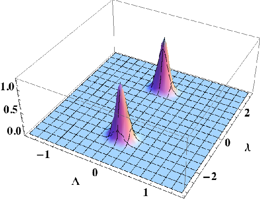
The classical phase quasi-distribution is then

p_{\mathrm{class}}(\lambda)=\int_{-\pi/2}^{\pi/2}\frac{d\Lambda}{2\pi}(\cos\Lambda)^{N-M}\left[\cos\Lambda+\cos\lambda\right]^{m_{1}}\left[\cos\Lambda-\cos\lambda\right]^{M-m_{1}}

(52)

A plot of this function for the same variable values is shown in Fig. 15. Only the two classical peaks survive here.

An interesting feature of the PO is that, while within the reduced probability of Eq. (51) one can replace $\Lambda$ by zero and get the classical limit, it is not correct in Eq. (44), which contains no factor $(\cos\Lambda)^{N-M}$ . The result is that one can still get strong populations oscillations and marked even-odd changes, even in the limit $M\ll N.$ The quantum angle $\Lambda$ therefore remains necessary even in this case.

Population oscillations can continue to exist under certain circumstances even if some particles are missed in the measurements; they are more robust in this respect than violations of locality. This point is discussed in Appendix A.

IV.2 Population oscillations with interference fringes in free space

We now attempt to reproduce the analysis of Dunningham et al. (DBRP) in Ref. [16] in which three Fock sources form an interference pattern in free space on a screen, while some of the particles are deflected near the sources by beam splitters, where they are counted. Fig. 16 shows the experimental arrangement considered. We will designate $M$ as the number of particles involved in the interference measurements made on the screen where interference takes place. Then the number of particles measured near the sources having initial particle numbers $N_{\alpha}=N_{\beta}=N_{\gamma}=N$ (as in the work of DBRP) will be $m_{\alpha}$ , $m_{\beta},$ and $m_{\gamma}$ ; these are the particles that did not take part in the interference pattern. All together then we will have measured

3N=M+m_{\alpha}+m_{\beta}+m_{\gamma}

(53)

particles. We can then write the probability as

P(m_{\alpha},m_{\beta},m_{\gamma},r_{1},\cdots,r_{M})\sim\left\langle\Gamma_{m_{\alpha}m_{\beta}m_{\gamma}M}\left|\Gamma_{m_{\alpha}m_{\beta}m_{\gamma}M}\right.\right\rangle

(54)

where

\left|\Gamma_{m_{\alpha}m_{\beta}m_{{}^{\gamma}}M}\right\rangle=\frac{a_{\alpha}^{m_{\alpha}}a_{\beta}^{m_{\beta}}a_{\gamma}^{m_{\gamma}}}{\sqrt{m_{\alpha}!m_{\beta}!m_{\gamma}!}}\prod_{i=1}^{M}(a_{\alpha}e^{ik_{\alpha}\cdot r_{i}}+e^{ik_{\beta}\cdot r_{i}}a_{\beta}+a_{\alpha}e^{ik_{\gamma}\cdot r_{i}})\left|N,N,N\right\rangle

(55)

To correspond with Ref. [16] we take $k_{\alpha}=k,$ $k_{\beta}=-k$ and with $k_{\gamma}=0$ .

We can introduce a vacuum state in between the $\left|\Gamma\right\rangle$ ’s and compute the matrix element by multiplying out the interference operators:

\displaystyle\left\langle 0\left|\right.\Gamma\right\rangle

\displaystyle=

\displaystyle\frac{1}{\sqrt{m_{\alpha}!m_{\beta}!m_{\gamma}!}\sqrt{N!^{3}}}\sum_{p}K_{p_{a}p_{\beta}p_{\gamma}}(r)\left\langle 0\left|a_{\alpha}^{m_{\alpha}+p_{\alpha}}a_{\beta}^{m_{\beta}+p_{\beta}}a_{\gamma}^{m_{\gamma}+p_{\gamma}}a_{\alpha}^{\dagger N}a_{\beta}^{\dagger N}a_{\gamma}^{\dagger N}\right|0\right\rangle

(56)

where $K_{p}$ is a coefficient that depends on the $r_{i}$ . The matrix element produces delta functions that can be replaced by integrals in our standard way. The results is

	$\displaystyle\left\langle 0\left\|\right.\Gamma\right\rangle$	$\displaystyle=$	$\displaystyle\frac{\sqrt{N!^{3}}}{\sqrt{m_{\alpha}!m_{\beta}!m_{\gamma}!}}\int\frac{d\lambda_{\alpha}}{2\pi}\int\frac{d\lambda_{\beta}}{2\pi}e^{-i(N_{\alpha}-m_{\alpha})\lambda_{\alpha}}e^{-i(N_{\beta}-m_{\beta})\lambda_{\alpha}}$		(57)
			$\displaystyle\prod_{i=1}^{M}(e^{ik\cdot r_{i}}e^{i\lambda_{\alpha}}+e^{-ik\cdot r_{i}}e^{i\lambda_{\beta}}+1)$		(57)

If we take the absolute square of this we introduce two new variables $\lambda_{\alpha}^{\prime}$ and $\lambda_{\beta}^{\prime}$ . We then make the following variable changes:

	$\displaystyle\lambda_{\alpha}$	$\displaystyle=$	$\displaystyle-\lambda+\frac{\Lambda}{2},\quad\lambda_{\alpha}^{\prime}=-\lambda-\frac{\Lambda}{2},$
	$\displaystyle\lambda_{\alpha}$	$\displaystyle=$	$\displaystyle\lambda^{\prime}+\frac{\Lambda^{\prime}}{2},\quad\lambda_{\beta}=\lambda+\frac{\Lambda^{\prime}}{2},$		(58)

The probability then becomes

$\displaystyle P(m_{\alpha},m_{\beta},m_{\gamma},r_{1},\cdots,r_{M})$	$\displaystyle=$	$\displaystyle\frac{N!^{3}}{m_{\alpha}!m_{\beta}!m_{\gamma}!}\int_{-\pi}^{\pi}\frac{d\lambda}{2\pi}\int_{-\pi}^{\pi}\frac{d\lambda^{\prime}}{2\pi}\int_{-\pi}^{\pi}\frac{d\Lambda}{2\pi}\int_{-\pi}^{\pi}\frac{d\Lambda^{\prime}}{2\pi}e^{-i(N-m_{\alpha})\Lambda}$	(59)
		$\displaystyle\times e^{-i(N-m_{\beta})\Lambda^{\prime}}\prod_{i=1}^{M}\left[1+e^{i\Lambda}+e^{i\Lambda^{\prime}}\right.$
		$\displaystyle+2\cos(2k\cdot r_{i}-\lambda-\lambda^{\prime})e^{i(\Lambda+\Lambda^{\prime})/2}$
		$\displaystyle+\left.2\cos(k\cdot r_{i}-\lambda)e^{i\Lambda/2}+2\cos(k\cdot r_{i}-\lambda^{\prime})e^{i\Lambda^{\prime}/2}\right]$

If we sum out the $m_{i}$ we find the probability for the $r-$ set under arbitrary source number detections:

$\displaystyle P(r_{1},\cdots,r_{M})$	$\displaystyle=$	$\displaystyle\frac{N!^{3}}{(3N-M)!}\int_{-\pi}^{\pi}\frac{d\lambda}{2\pi}\int_{-\pi}^{\pi}\frac{d\lambda^{\prime}}{2\pi}\int_{-\pi}^{\pi}\frac{d\Lambda}{2\pi}\int_{-\pi}^{\pi}\frac{d\Lambda^{\prime}}{2\pi}e^{-iN(\Lambda+\Lambda)}$	(60)
		$\displaystyle\times\left(1+e^{i\Lambda}+e^{i\Lambda^{\prime}}\right)^{3N-M}$
		$\displaystyle\times\prod_{i=1}^{M}\left[1+e^{i\Lambda}+e^{i\Lambda^{\prime}}+2\cos(2k\cdot r_{i}-\lambda-\lambda^{\prime})e^{i(\Lambda+\Lambda^{\prime})/2}\right.$
		$\displaystyle+\left.2\cos(k\cdot r_{i}-\lambda)e^{i\Lambda/2}+2\cos(k\cdot r_{i}-\lambda^{\prime})e^{i\Lambda^{\prime}/2}\right]$

The integral method above is not very useful for simulations. We have developed a recurrence method in which the wave function for $R$ measurements is written in terms of that for $R-1$ measurements. We do not give details here to save space. All the probabilities $p(m_{\alpha},m_{\beta})$ for finding particles in the source detectors for a given set of positions $r_{1},\cdots,r_{M}$ (with $m_{\gamma}$ given by Eq. (53)) are computed in a single recurrence run. We show a plot in Fig. 17 of the resulting population oscillation ridges. DBRP found that the ridges were parallel to one axis shown in their Fig. 5. Indeed our ridges are parallel to $m_{\gamma}=$ constant, which would have been more obvious had we plotted using, say, the $m_{\alpha},m_{\gamma}$ axes. The parallel axis in our case is the one having the intermediate vector $(k_{\gamma}=0)$ so that we are in agreement with the results of DBRP.

V Conclusion

In many cases, such as for instance the description of the MIT experiment [1] with initial Fock states, introducing a classical relative phase angle $\lambda$ is sufficient. Cases exist, nevertheless, where the classical phase is not able to explain all quantum predictions, and where introduction of the quantum angle $\Lambda$ (or its equivalent) becomes necessary. We have discussed two examples, in Secs. III and IV, where interesting physical effects can not be understood only in terms of the classical phase. In both cases, quantum effects are related to peaks of the function $F(\lambda,\Lambda)$ in the “quantum region” (i. e., away from $\Lambda=0$ ), and disappear completely if $\Lambda$ is set to zero.

In the first double interferometer experiment, we find violations of the BCHSH inequalities and therefore violations of locality. Setting the quantum angle to zero reduces the equations to purely classical equations, which could be interpreted as being integrated over a hidden variable as in Bells theorem. Only the quantum angle leads to the violations.

In the population oscillation experiment, we find that simultaneous measurements of “non-commuting variables” phase and particle number within the same apparatus yield oscillations in measurements of the number variable that are a direct result of the off-diagonal phase (i. e., quantum) peaks and provide an example of QIMDS. However, as discussed in Appendix B, one can replace the measurement of the phase by that of the parity, which does not fix the relative phase of the two condensates at all; but this does not completely cancel the population oscillations since the central dark fringe remains present with a 100% contrast, while the characteristics of the superposition are completely changed (the “phase cat” becomes completely “blurred”). The fact that some population oscillations remain visible, at least for the first fringe, illustrates that the PO can exist more generally than with just the coherent superpositions of different macroscopic phases.

The two experiments we have discussed are of somewhat different nature. The former exhibits strong quantum non-locality effects, while for the latter we have not found violations of the Bell inequalities. Nevertheless, while for the former the violations of the inequalities require that all particles are measured (they disappear as soon as a single particle is missed), the population oscillations are a manifestation of the quantum angle that is more robust as we show in Appendix A; they can still exist, although in a more limited way, when a few particles are missed.

Acknowledgements.

We wish to thank the authors of Ref. [16], J. A. Dunningham, K. Burnett, R. Roth and W. D. Phillips, as well as A. Smerzi and A. Piazza, for interesting and helpful comments and discussions.

APPENDICES

V.1 Incomplete measurements in the PO experiment

V.1.1 No phase measurements

We study the experiment of Fig. 7 again, but now assume that no measurement is performed in the interference region D, and that only the population measurements are performed; then, whether or not a beam splitter is used in this regions does not matter anymore). We then have to sum the probabilities (44) over $m_{1}$ and $m_{2}$ , with a constant sum $m_{1}+m_{2}=M$ . The summation introduces the $M$ -th power of a binomial $[e^{i\Lambda}+e^{-i\Lambda}]$ , but only one term of this power survives the $\Lambda$ integration; we then obtain

\sum_{m_{1}+m_{2}=M}P(m_{1},m_{2},m_{\alpha},m_{\beta})=\frac{N_{\alpha}!N_{\beta}!}{m_{\alpha}!m_{\beta}!\,2^{N-M}}\frac{M!}{p!(N-p)!}

(61)

with $p$ defined by

2p=N_{\alpha}-m_{\alpha}-N_{\beta}+m_{\beta}

(62)

(one can easily check that the right hand side of this equation is an even number). The $\lambda$ integral has now disappeared, as expected since no measurement of the relative phase is made. Moreoever, the probability factorizes as expected since, in the absence of interference measurements, two completely independent experiments are performed in different regions of space: in each region, the transmission or reflection of the particles on the beam splitter are independent random processes.

V.1.2 No population measurements

Conversely, assume that all population measurements are ignored and that only the interference measurements are considered. The corresponding probability is then

	$\displaystyle\sum_{m_{\alpha}+m_{\beta}=N-M}P(m_{1},m_{2},m_{\alpha},m_{\beta})$	$\displaystyle=$	$\displaystyle\frac{N_{\alpha}!N_{\beta}!}{(N-M)!m_{1}!m_{2}!2^{M}}\int_{-\pi}^{\pi}\frac{d\lambda}{2\pi}\int_{-\pi}^{\pi}\frac{d\Lambda}{2\pi}\,[\cos\Lambda]^{N-M}$		(63)
			$\displaystyle\times\left[\cos\Lambda+\cos\lambda\right]^{m_{1}}\left[\cos\Lambda-\cos\lambda\right]^{m_{2}}$		(63)

Now the phase $\lambda$ no longer disappears, but combines its effects with the quantum angle $\Lambda$ ; the $[\cos\Lambda]^{N-M}$ introduces a peaking function around the origin, which may behave similarly to a delta function if $N-M$ is sufficiently large. We now discuss the interplay between the classical phase and the quantum angle $\Lambda$ .

V.1.3 Missed particles

Next suppose some of the particles are lost and not measured in either interferomenter nor side detectors of Fig. 7. We have seen in the case of the double interferometer Bell-violation experiment that a single missed particle can remove any locality violations. We simulate these lost particles in the PO experiment by putting additional side detectors as shown in Fig. 18. Assume that the beam splitters at detectors 5 and 6 each have a transmission coefficient $T.$

We assume that particle losses $m_{5}$ and $m_{6}$ are known to total $M_{L}$ , but the individual numbers are not actually recorded. Thus to get the probability we are interested in we must sum over all $m_{5}$ and $m_{6}$ adding to the total $M_{L}$ . Proceeding as in Sec. IV we find

	$\displaystyle P(m_{1},m_{2},m_{\alpha},m_{\beta})$	$\displaystyle=$	$\displaystyle\frac{N_{\alpha}!N_{\beta}!T^{N-M_{L}}(R)^{M_{L}}}{m_{1}!m_{2}!m_{\alpha}!m_{\beta}!2^{N-2M_{L}}M_{L}!}\int_{-\pi}^{\pi}\frac{d\lambda}{2\pi}\int_{-\pi}^{\pi}\frac{d\Lambda}{2\pi}\cos\left[\left(N_{\alpha}-m_{\alpha}-N_{\beta}+m_{\beta}\right)\Lambda\right]$		(64)
			$\displaystyle\times\cos(\Lambda)^{M_{L}}\left[\cos\Lambda+\cos\lambda\right]^{m_{1}}\left[\cos\Lambda-\cos\lambda\right]^{m_{2}}$		(64)

with $R=1-T.$ The result of the lost particles is the factor $\cos(\Lambda)^{M_{L}},$ which, if $M_{L}$ is large enough, diminishes the quantum peaks, as we have seen before as in, say, Eq. (63). The result maintains the same form if we also allow particles to be missed elsewhere in the device, say, after the beam splitter at detectors 1 and 2.

If we count $N_{D}=m_{1}+m_{2}+m_{\alpha}+m_{\beta}$ particles in the real detectors but $M_{L}$ were missed in one place or another in the device, then we must have had $N=N_{D}+M_{L}$ particles in the sources originally. The missed particles could have come from source $\alpha$ or source $\beta$ . We assume that the sources originally have $N_{\alpha}=\bar{N_{\alpha}}+\Delta_{\alpha}$ and $N_{\beta}=\bar{N_{\beta}}+\Delta_{\beta}$ where $\bar{N_{\alpha}}+\bar{N_{\beta}}=N_{D}$ and $M_{L}=\Delta_{\alpha}+\Delta_{\beta}$ . We first fix $M_{L}$ and sum over all possible $\Delta_{\alpha}$ and then sum over all $M_{L}$ in principle from 0 to $\infty$ . If $R$ is small, then the sum over $M_{L}$ should converge after a reasonably small number of missed particles. That is, the probability of missing $X_{L}$ particles, where $X_{L}$ is very large is negligible. One would hope that if $R$ is small enough, then the PO will converge to a situation in which the fringes are not lost. We find this to be the case under certain conditions. We can also find the average number of particles lost by multiplying the probability by $M_{L}$ and summing over all $\Delta_{\alpha}$ , $M_{L},$ and $m_{\alpha.}$

Consider the situation with $m_{1}=17$ and $m_{2}=83.$ The PO for the cases with $T=0.98$ and $T=0.99$ are shown in Fig. 19. For $T=0.98$ the oscillations are completely removed and for 0.99 only a remnant is left. In the later case we have lost 3.8 particles on average.

The smaller the value of $m_{1}$ , the closer in to $\Lambda=0$ are the off-diagonal peaks in $F(\Lambda,\lambda)$ so that they get less blotted out by the $\cos\Lambda^{M_{L}}$ factor. If we lower $m_{1}$ to 3 we find the results in Fig. 20. We still lose the central dip in the PO diagram for $T=0.98,$ but for $T=0.99,$ we get a much deeper remnant.

To what degree must we restrict losses to guarantee that we would have more than a single dip? Fig. 21 shows the case of $N=200,$ $m_{1}=17$ with the transmission coefficient up to $T=0.997.$ Only 1.4 particles have been lost here. For smaller $m_{1}$ values one gets deeper central dips, but not the dips on the side for the same $T$ values.

V.2 Measuring the parity

Fig. 10 shows that the $\Lambda$ peaks in the quantum region have a sign that depends on the parity of $m_{1}$ or $m_{2}$ , which suggests that a possible method to observe the population oscillations is to associate them with a measurement of the parity at the interferometer, instead of the relative phase of the two condensates.

Fig. 22 illustrates what is obtained if, for instance, one adds the probabilities associated with all odd values of $m_{1}$ . The left part of the figure shows the variations of $F(\Lambda,\lambda)$ , the right part the associated population oscillation as a function of $m_{1}$ , with $m_{2}=40-m_{1}$ . One notices the disappearance of the two peaks that characterized the coherent superposition of two values of the relative phase; they are now replaced by a more delocalized structure, similar to a ridge. In other words, the “Schrödinger cat” is now spread over many values of the phase. But one also sees in the right part that the populations oscillations still exist, with a central dark fringe that has 100% contrast when $m_{\alpha}$ varies only by one unit; the variation is actually not very different from the right part of Fig. 13, except of course the change of sign due to the change of parity of $m_{1}$ . This shows that the central fringe of the population oscillations is not specifically related to a measurement of the phase, or to the existence of any “Schrödinger cat”; it continues to exist if a very different physical quantity is measured, such as the parity, which does not give any particular information on the relative phase of the two condensates.

V.3 Two phase measurements

In the population oscillation experiment, we have considered the use of a single interferometer; we can generalize this experiment to two interferometers each of which have different settings, $\zeta$ and $\theta$ . We begin with the device in Fig. 5 and add to that the side detectors shown in Fig. 7, to allow phase-type measurements in two different regions of space as well as population measurements near the two sources. The resulting apparatus is shown in Fig. 23.

The calculations proceed as in previous sections and lead to a result for the probability of finding the series of results $\{m_{1},m_{2},m_{3},m_{4},m_{\alpha},m_{\beta}\}$ equal to

$\displaystyle\mathcal{P}(m_{1},m_{2},m_{3},m_{4},m_{\alpha},m_{\beta})$	$\displaystyle=$	$\displaystyle\frac{N_{\alpha}!N_{\beta}!}{2^{M}N!m_{1}!\cdots m_{4}!m_{\alpha}!m_{\beta}!}\int_{-\pi}^{\pi}\frac{d\lambda}{2\pi}\int_{-\pi}^{\pi}\frac{d\Lambda}{2\pi}$	(65)
		$\displaystyle\times\cos\left[(N_{\alpha}-N_{\beta}-m_{\alpha}+m_{\beta})\Lambda\right]$
		$\displaystyle\times\prod_{i=1}^{4}\left[\cos\Lambda+\eta_{i}\cos\left(\lambda+\varphi_{i}\right)\right]^{m_{i}}$

where $M=m_{1}+\cdots+m_{4},$ $\eta_{1}=\eta_{3}=1$ ; $\eta_{2}=\eta_{4}=-1$ ; $\varphi_{1}=\varphi_{2}=-\zeta$ ; $\varphi_{3}=\varphi_{4}=\theta$ . This result is essentially the same as Eq. (20) with the addition now of the cosine transform in $\Lambda.$ This factor allows population oscillations as in Sec. IV. However now we have the option of adjusting relative phases between the two interferometer sets.

A summation version of the probability is much more convenient for computing population oscillations. A result analogous to Eq. (40) of Sec. IV is

$\displaystyle\mathcal{P}(m_{1},m_{2},m_{3},m_{4},m_{\alpha},m_{\beta})$	$\displaystyle=$	$\displaystyle\frac{m_{1}!\cdots m_{4}!}{m_{\alpha}!m_{\beta}!2^{N+2M}}\sum_{p_{2}p_{3}p_{4}}\frac{(-1)^{p_{2}+p_{4}}e^{-i(\zeta+\theta)(p_{3}+p_{4})}}{p_{2}!p_{3}!p_{4}!(m_{2}-p_{2})!(m_{3}-p_{3})!(m_{4}-p_{4})!}$	(66)
		$\displaystyle\times\frac{1}{(N_{\alpha}-m_{\alpha}-p_{2}-p_{3}-p_{4})!}$
		$\displaystyle\times\frac{1}{(m_{1}-N_{\alpha}+m_{\alpha}+p_{2}+p_{3}+p_{4})!}$

Because two independent settings $\theta$ and $\zeta$ are now available, the phase sign ambiguity can be removed. As a consequence, by adjusting the phase angles on the interferometers, we can now control the relative sizes of the two classical peaks, i. e., those along $\Lambda=0$ . Consider the following plots where we show the last line of the integrand of Eq. (65) and the population oscillations given by Eq. (66) associated with the same parameters. With the phase shifters set at zero the two classical peaks have equal sizes and there is a definite population oscillation structure (Fig. 24). However, with a different phase shift, one of the classical peaks can be made much smaller as seen in Fig. 25 and the quantum peaks become smaller as well. Moreover, the population oscillation central zero no longer vanishes. For other phase shift angles (for instance $\zeta=0$ and $\theta=2.5$ radian), the integrand can be reduced to a single classical peak with no peak in the quantum region at all; the corresponding population oscillation central dip then becomes a simple peak.

If the state vector is the sum of two components centered around two different values of the phase, and if the norm of one component is larger than that of the other, one obtains two peaks in the classical region, one large and one small. The small classical peak corresponds to a population in the phase representation, so that it is second order with respect to the second component of the state vector. By contrast, the peaks in the quantum region are first order, since they correspond to off-diagonal matrix elements. As a consequence, when one reduces the small phase component, the small classical peak disappears more rapidly than the quantum peaks. This explains why the left of Fig. 25 has a classical peak that is barely visible, but still clearly shows the (negative) quantum peaks.

References

[1] M. R. Andrews, C. G. Townsend, H.-J. Miesner, D.§. Durfee, D. M. Kurn, W. Ketterle, Science, 275, 637 (1997).
[2] C. Pethick and H. Smith, Bose-Einstein Condensation in Dilute Gases, Cambridge University Press (2001).
[3] J. Javanainen and Sun Mi Yoo, Phys. Rev. Lett. 76, 161-164 (1996).
[4] T. Wong, M. J. Collett and D. F. Walls, Phys. Rev. A $\mathbf{55}$ , 1288 (1997).
[5] J. I. Cirac, C. W. Gardiner, M. Naraschewski and P. Zoller, Phys. Rev. A $\mathbf{54}$ , R3714 (1996).
[6] Y. Castin and J. Dalibard, Phys. Rev. A $\mathbf{55}$ , 4330 (1997).
[7] K. Mølmer, Phys. Rev. A $\mathrm{\mathbf{55}}$ , 3195 (1997).
[8] K. Mølmer, J. Mod. Opt. $\mathbf{44}$ , 1937 (1997)
[9] F. Laloë, Europ. Phys. J. D 33, 87 (2005); see also arXiv:cond-mat/0611043v1.
[10] F. Laloë and W.J. Mullin, Phys. Rev. Lett. 99, 150401 (2007); Phys. Rev. A 77, 022108 (2008).
[11] W.J. Mullin, R. Krotkov, and F. Laloë, Amer. J. Phys. 74, 880 (2006).
[12] J.S. Bell, Physics 1, 195 (1964), reprinted in J.S. Bell, Speakable and Unspeakable in Quantum Mechanics, (Cambridge University Press, Cambridge, 1987).
[13] A. Einstein, B. Podolsky and N. Rosen, Phys. Rev. 47, 777-780 (1935).
[14] W.J. Mullin and F. Laloë , Phys. Rev. A, 78, 061605(R) (2008).
[15] F. Laloë and W.J. Mullin, Europ. Phys. J. B $\mathbf{70}$ , 377 (2009); arXiv:0812.1592.
[16] J. A. Dunningham, K. Burnett, R. Roth, and W. D. Phillips, New J. of Phys. 8, 182 (2006).
[17] W. J. Mullin and F. Laloë, Phys. Rev. Lett. XXXXX
[18] A. J. Leggett, Supple. Prog. Theor. Phys. 69, 80-100 (1980); J. Phys: Condens. Matter $\mathbf{14}$ , R415-R451 (2002); Physica Scripta, $\mathbf{T102}$ , 69 (2002).
[19] F. Laloë and W.J. Mullin, arXiv:1004.1731v1
[20] J. F. Clauser, M. A. Horne, A. Shimony, and R. A. Holt, Phys. Rev. Lett. 23, 880 (1969).
[21] M. J. Holland and K. Burnett, Phys. Rev. Lett. 71, 1355 (1993)
[22] J. Franson, Phys. Rev. A 49, 3221 (1994).
[23] S.M. Barnett and D.T. Pegg, Phys. Rev. A 42, 6713 (1994).
[24] A. Dragan and P. Zin , Phys. Rev. A $\mathbf{76}$ , 042124 (2007).