Dissipation in a rotating frame: master equation,
effective temperature and Lamb-shift

In the microscopic model for quantum dissipation a quantum mechanical system is coupled to a thermal bath so that the total Hamiltonian takes the form $H=H_{S}+H_{B}+H_{I}$ with $H_{S}$ being the Hamiltonian of the bare system, $H_{B}$ the Hamiltonian of the heat bath, and $H_{I}$ the interaction, i.e.,

The time evolution of the density matrix of the full compound $W(t)$ obeys the Liouville-von Neumann equation $i\hbar d{W}(t)/dt=[H,W(t)]$ with an initial state $W(0)$. The relevant operator is the reduced density $\rho(t)={\rm tr}_{B}\{W(t)\}$ for which a simple equation of motion does in general not exist. In case of weak friction and sufficiently fast bath modes, however, progress is made within a Born-Markov approximation. One then obtains the usual master equation which we cast in the form

where

contains the position operator $q(s)$ in the interaction representation and $\{,\}$ denotes the anti-commutator. The effective impact of the bath appears as a force-force correlator $K(t)=1/\hbar\langle\xi(t)\xi(0)\rangle_{\beta}=K^{\prime}+iK^{\prime\prime}$ with $\xi=\sum c_{n}x_{n}$,

including the spectral density $I(\omega)=\frac{\pi}{2}\sum_{n}\frac{c^{2}_{n}}{m_{n}\omega_{n}}\delta(\omega-\omega_{n})$ of the bath modes. Processes mediated by these modes are revealed most clearly in the representation of the master equation using the eigenstates of the bare system $H_{S}|n\rangle=E_{n}|n\rangle$. An additional rotating wave (or secular) approximation (RWA), where off-resonant (fast oscillating) terms in (2) are neglected, gives

First, the reservoir induces transitions between eigenstates with rates $\gamma_{nm}=|\langle n|q|m\rangle|^{2}\,D(\omega_{nm})$ at frequencies $\omega_{nm}=(E_{n}-E_{m})/\hbar$ where

with $n_{\beta}(\omega)=1/[\exp(\beta\hbar\omega)-1]$. The decay rates for the off-diagonal elements of the density matrix

contain the collective rates $\Gamma_{mm}=\sum_{k\neq m}\gamma_{km}$. Second, oscillation frequencies are renormalized $\tilde{\omega}_{nm}=\omega_{nm}+\Delta\omega_{nm}$ by the so-called Lamb-shift

The bath appears in form of

determined by

Moreover, $M$ denotes the mass of the system particle and $\eta_{\rm sin}$ is the $\sin$-transform of the classical friction kernel $\eta(t)=\int d\omega I(\omega)\cos(\omega t)/M\pi\omega$.

Since the environment rests in thermal equilibrium its probabilities $D(\omega)$ to emit and $D(-\omega)$ to absorb photons are related by detailed balance, i.e.,

This latter condition can also be used to define the temperature $\beta=1/k_{\rm B}T$ imposed asymptotically (for long times) by the bath onto the thermal state of the system: the stationary populations $P_{n}=\rho_{nn}$ of the system obey $P_{n}/P_{k}=D(-\omega_{nk})/D(\omega_{nk})$, thus leading to the known Boltzmann distribution.

We now consider a system with a standard Hamiltonian $H_{S}=p^{2}/2M+V(q)$ where in

a harmonic term is splitted off from anharmonic contributions. This system is subject to external periodic driving with frequency $\omega_{D}$. Then, asymptotically the reduced density does not reach thermal equilibrium, but rather approaches a time dependent state with periodicity $T_{F}\equiv 2\pi/\omega_{F}$. For instance, the standard dipole coupling between system and driving force $\propto q\cos(\omega_{D}t)$[7] leads to $\omega_{F}=\omega_{D}$, while a parametric driving of the form $\propto\cos(\omega_{D}t)q^{2}$ [10] gives rise to period doubling $\omega_{F}=\omega_{D}/2$. As already noted above, particularly the former situation is relevant for mesoscopic detectors built with microwave-driven JJ. The domain where the detector is most sensitive, is located around the first bifurcation threshold, where the anharmonicity $V_{1}$ is still weak and $(\omega_{0}-\omega_{D})/\omega_{0}\ll 1$. When amplitude and/or frequency of the external drive are tuned into this regime, after a transient period of time the density takes the form $\rho(t)\sim{\bar{\rho}}(t)\cos(\omega_{F}t)$ with $\bar{\rho}$ changing only slowly in time, i.e., on time scales $t\gg 1/\omega_{F}$. In principle, to derive the master equation for $\bar{\rho}$, one may follow the strategy outlined above, however, only after switching to a moving frame. We mention in passing that this mapping is closely related to a representation within Floquet theory [7] combined with a projection onto the subspace of the leading harmonics $\sim\exp(\pm i\omega_{F}t)$.

For this purpose, we introduce a unitary operator of the composite system

where $\hat{a}$ and $\hat{b}_{n}$ are annihilation operators for harmonic oscillators in the system and in the bath, respectively. The total Hamiltonian in the rotating frame

follows upon discarding fast oscillating terms $\exp(\pm ik\omega_{F}t)\,,|k|\geq 1$ as a time-independent Hamiltonian of the form $\tilde{H}_{S}(Q,P)=U_{S}^{{\dagger}}{\cal H}_{S}\,U_{S}$ and

The operator ${\cal H}_{S}=H_{S}-i\hbar\partial_{t}$ coincides with the extended Hamiltonian in the Floquet description so that the spectrum of $\tilde{H}_{S}$ reproduces the corresponding Floquet quasi-energies. Its eigenstates $|\tilde{\psi}_{n}\rangle$ are related to the Floquet states $|{\psi}_{n}\rangle$ via $|\tilde{\psi}_{n}\rangle=P_{F}U_{S}|{\psi}_{n}\rangle$ with $P_{F}$ being the projector onto the $(k\cdot\omega_{F})$-subspace with $k=\pm 1$. We emphasize that the original Hamiltonian (1) cannot be regained from (14) in the limit $\omega_{F}\to 0$ since then fast oscillating terms neglected in the derivation of (14) contribute.

For the derivation of the master equation the specific form of $\tilde{H}_{S}$ is not relevant. Important are the new bath parameters

Further, in the rotating frame the system-bath coupling is not just a position-position interaction but includes also the momenta, a point which we will discuss in more detail below. Starting now with $i\hbar d\tilde{W}/dt=[\tilde{H},\tilde{W}]$ and following the standard procedure, one obtains the master equation in the rotating frame

Here operators ${{\cal L}}_{QQ}$ and ${{\cal L}}_{PP}$ are defined according to (3) with $q$ replaced by ${Q},{P}/(\omega_{F}M)$ with the force-force correlator defined by

where

Whereas the mixed operators are

and ${\cal L}_{PQ}$ is defined according to (18) with $Q\leftrightarrow P$. The force-force correlators can be expressed as

and

with the spectral density in the rotating frame

Note that the unitary transformation (13) does not affect the equilibrium density of the bath since $[U_{B},H_{B}]=0$, but just the dynamics of the correlator. Accordingly, equilibrium properties in (19) appear through a frequency shift $\omega\to\omega-\omega_{F}$ meaning that in the rotating frame the bath carries modes with ”negative” frequencies. The above analysis shows that in the rotating frame a typical friction strength is given by $\tilde{\eta}={I}(\omega_{F})/4M\omega_{F}$ which is smaller than that in the lab frame $\eta=\lim_{\omega\to 0}I(\omega)/M\omega$. The frequency shift in the bath correlation function $\tilde{K}(t)$ effectively produces a decay in time which qualitatively is similar to that of $K(t)$. The condition for the validity of the master equation (15) can thus be estimated to read $\tilde{\eta}\hbar\beta\ll 1$ provided a typical bath cut-off frequency $\omega_{c}$ sufficiently exceeds $\eta>\tilde{\eta}$.

It is instructing to express the above master equation in terms of annihilation and creation operators. This is most conveniently done in the interaction picture representation where the reduced density is given by $\bar{\rho}_{I}(t)=e^{i\tilde{H}_{S}t/\hbar}\bar{\rho}(t)e^{-i\tilde{H}_{S}t/\hbar}$. This way, (15) translates into

We now introduce operators

where the sum runs over all energy eigenstates $|E\rangle$, $|E^{\prime}\rangle$ of $\tilde{H}_{S}$ with fixed energy difference $\hbar\omega$. $a$ and $a^{\dagger}$ are annihilation and creation operators of a harmonic oscillator with frequency $\Omega$, i.e.,

The above frequency dependent operators satisfy $[\tilde{H}_{S},a^{\dagger}(\omega)]=\hbar\omega a^{\dagger}(\omega)$ and $[\tilde{H}_{S},a(\omega)]=-\hbar\omega a(\omega)$ and are thus creation and annihiliation operators at frequency $\omega$. Note that these relations hold independent of the frequency $\Omega$ in the definition (24). For a purely harmonic system with frequency $\tilde{\omega}_{0}$, however, the $a^{\dagger}(\omega),a(\omega)$ reduce to $a,a^{\dagger}$ only if $\Omega=\tilde{\omega}_{0}$. It is thus convenient to chose $\Omega$ as the frequency of small oscillations around one of the stable extrema of $\tilde{H}_{S}$, for instance that one where the dynamics starts initially.

The sum of dissipative operators in (21) can now be expressed as

with

Here, the Laplace transforms of the damping kernel (19) follow from

and the impact of the momentum dependent coupling terms between system and bath are taken into account by coefficients

As for the standard case, a further simplification arises within the RWA, where all terms in the sum (26) with $\omega\neq\omega^{\prime}$ are assumed to oscillate so rapidly on the time scale for relaxation that they may be discarded. Accordingly, (26) reduces to

We recall that the anharmonicity of the system potential gives rise to the frequency sum. In contrast, for a purely harmonic system with frequency $\Omega=\tilde{\omega}_{0}$ it collapses to contributions for $\omega=\pm\Omega$. Moreover, $a(-|\omega|)=a^{\dagger}(-|\omega|)=0$ so that terms carrying in (26) the coefficient $\lambda^{+}$ vanish. One should emphasize that this is not the case if in (24) a frequency $\Omega\neq\tilde{\omega}_{0}$ is chosen. A conventional master equation then emerges with renormalized friction functions $\hat{K}^{\prime}\to(\lambda^{-}\hat{K}_{QQ}^{\prime}-\mu\hat{K}_{QP}^{\prime\prime})$ and $\hat{K}^{\prime\prime}\to(\lambda^{-}\hat{K}_{QQ}^{\prime\prime}+\,\mu\hat{K}_{QP}^{\prime})$. In the Wigner representation the momentum coupling terms ensure that in the laboratory frame the known Fokker-Planck equation for driven systems is reproduced. To neglect them in the rotating frame leads in turn to spurious diffusion terms in the lab frame [17].

In the anharmonic case and for elevated temperatures it may be more convenient not to work explicitly with annihilation/creation operators, but rather use a representation as in (5), where matrix elements of those system operators appear which couple to the bath. In particular, these matrix elements can then directly be evaluated for the full anharmonic problem by means of semiclassical techniques in certain ranges of parameter space [10, 18]. The standard result can easily be generalized to the rotating frame situation: in addition to matrix elements $\langle m|Q|n\rangle$ also $\langle m|P/M\omega_{F}|n\rangle$ must be taken into account; these matrix elements are multiplied by the bath correlation functions $\tilde{D}_{xy}$ and $\tilde{D}_{xy}^{L}$ derived from $\tilde{K}_{xy}$. The diagonal part of the density $\bar{\rho}$ thus obeys a Pauli-master equation with properly modified transition rates,

If typical transition frequencies in $\tilde{H}_{S}$ are small compared to the driving frequency $\omega_{F}$ the dominant process in the transition rates is given by the position matrix element. For instance, close to a harmonic minimum with frequency $\tilde{\omega}_{0}$ and near the bifurcation threshold the momentum dependent terms provide contributions which are suppressed by factors on the order of $\tilde{\omega}_{0}/\omega_{F}\ll 1$.

As already mentioned above, the RWA does not always apply. For instance, for higher lying states the energy spectrum of $\tilde{H}_{S}$ may have accumulation points with a dense distribution of transition frequencies. This issue becomes particular relevant for the situation described above, namely, a driven system close to its first bifurcation threshold. Then typically $\tilde{H}_{S}$ exhibits two stable domains in phase space which are separated by an unstable one, as e.g. for parametric driving where one has a double well structure with the two minima corresponding to the stable extrema and the barrier top to an unstable saddle point of the dynamics. Accordingly, for sufficiently deep wells the RWA applies for low lying states. By tuning the system close to a bifurcation point, however, extrema tend to coalesce so that the spectrum of $\tilde{H}_{S}$ becomes narrowly spaced and the RWA is no longer applicable.

The model described by (14) can be considered as a system subject to relaxation as in the standard situation. Effectively for long times the bath dictates its temperature to the system such that the populations of the quasi-energy levels become stationary and are distributed according to a balance between emission and absorption processes. In case of a purely harmonic system the corresponding stationary populations can be calculated explicitly [17]. For the anharmonic case they follow within the RWA from the extended Pauli-master equation. It is thus convenient to introduce the concept of an effective temperature, which is defined according to (12) by $\exp(-\beta_{xy}\hbar\omega)=\tilde{D}_{xy}(-\omega)/\tilde{D}_{yx}(\omega)$, with $x,y=Q,P$. Now, a quantum of energy $\hbar\omega\geq 0$ emitted from the system reaches the bath in the lab frame either with energy $\hbar\omega_{+}=\hbar(\omega_{F}+\omega)$ or $\hbar\omega_{-}=\hbar(\omega_{F}-\omega)$, thus determining two distinct regimes. In the range $\omega>\omega_{F}$ only $\omega_{+}>0$ so that only one channel of bath modes is accessible and one unique effective temperature follows from the standard expression with a shifted frequency

The situation is different in the second range $\omega<\omega_{F}$ where both frequencies $\omega_{\pm}>0$ and two channels in the bath are open to give different effective temperatures for different diffusion processes, namely,

and from (19) and (20) also $\beta_{QQ}^{<}=\beta_{PP}^{<}$ and $\beta_{QP}^{<}=\beta_{PQ}^{<}$.

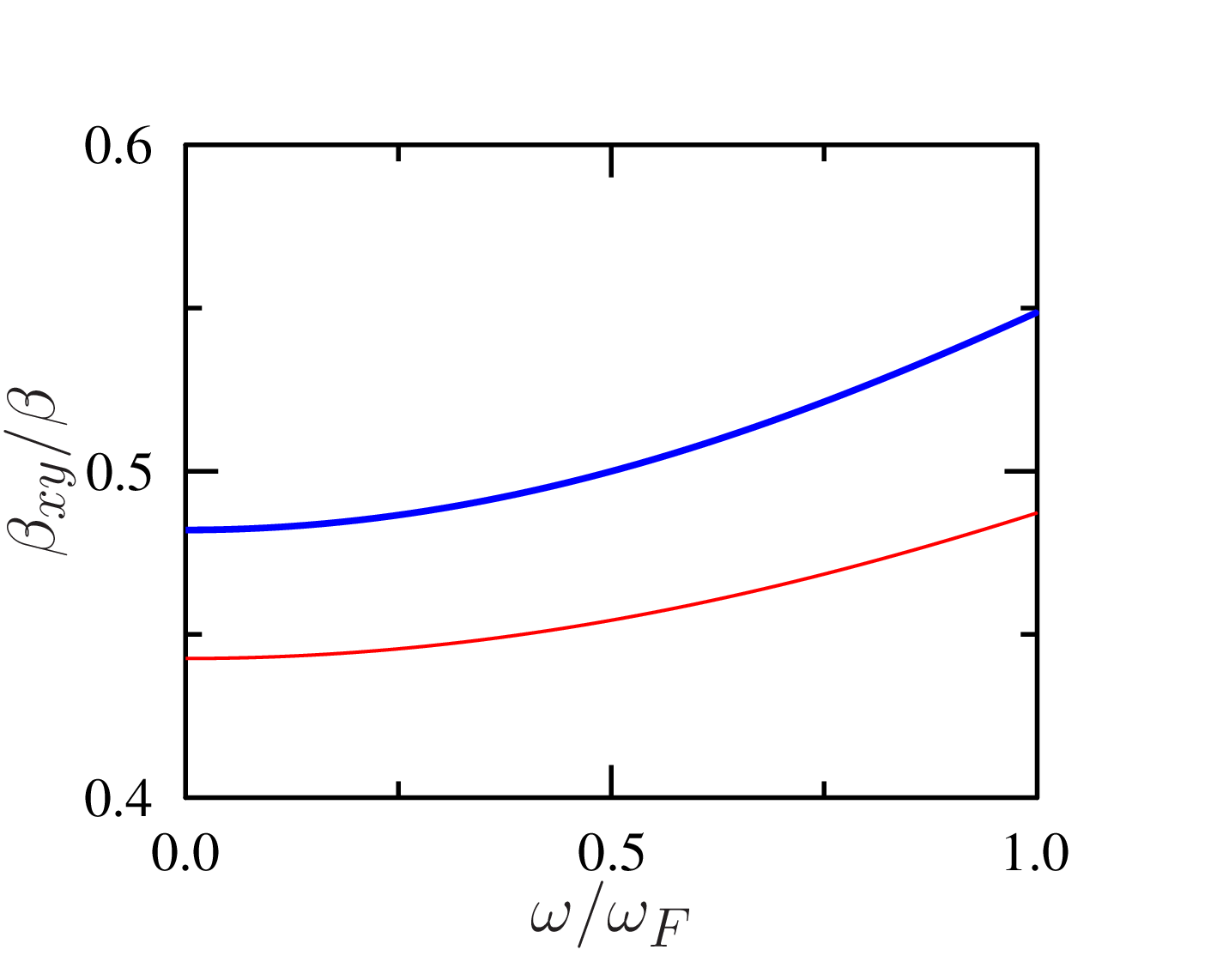
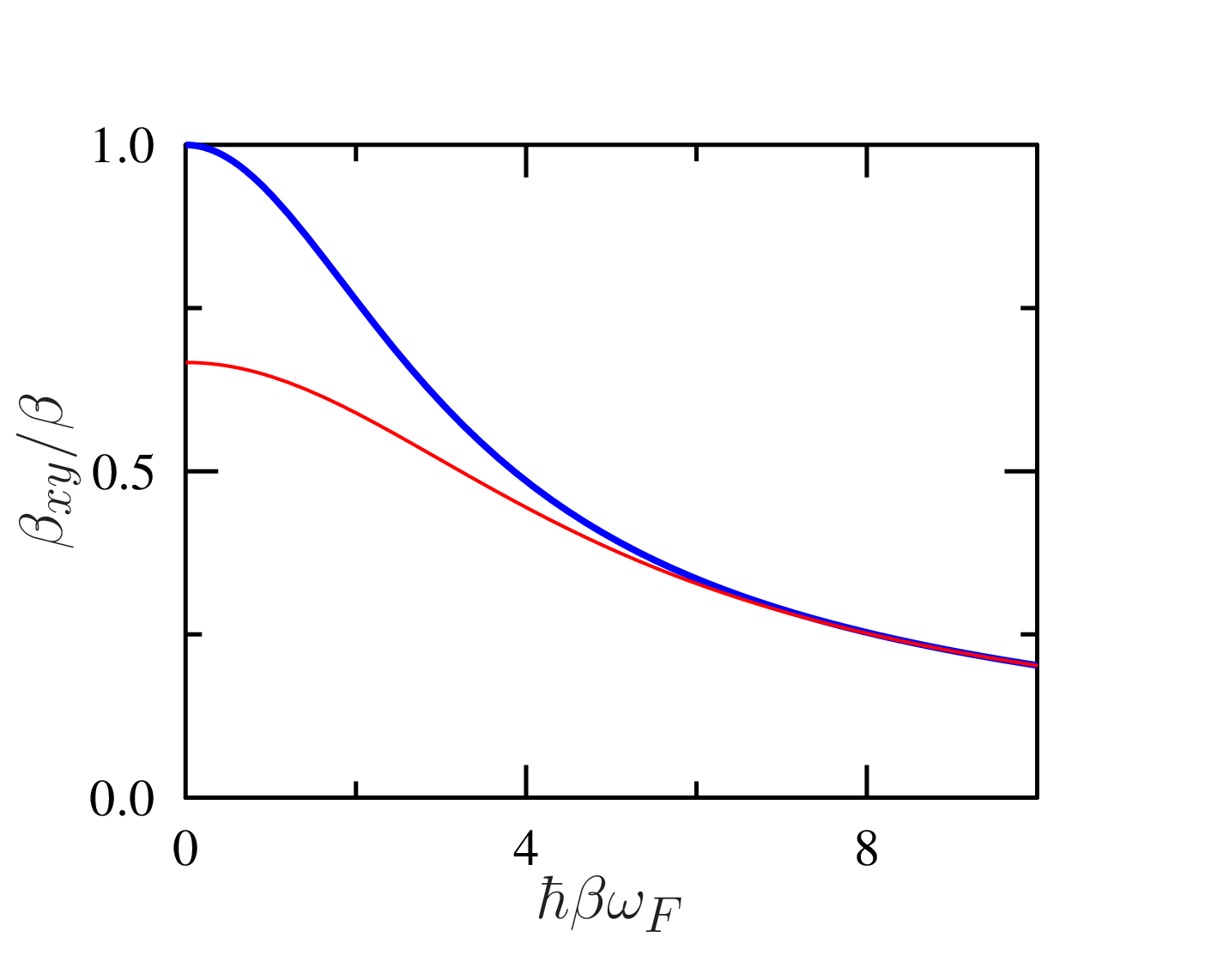
These results are illustrated in (fig.2-2). Apparently, the different combinations of the two channels lead to $\beta_{QQ}^{<}\neq\beta_{QP}^{<}$ so that a unique effective temperature cannot be specified, which in turn means that a detailed balance relation does in general not exist in the rotating frame. Only if the temperature tends to zero, i.e. $\omega_{F}\hbar\beta\gg 1$, do the individual effective temperatures merge (see fig.2) so the detailed balance is reestablished.

Let us now discuss the situation in more detail. First, while one recovers for vanishing rotating frame frequency $T_{xy}^{>}=T_{xy}^{<}=T$, for finite $\omega_{F}$ a discontinuity occurs $T_{xy}^{<}(\omega_{F})>T_{xy}^{>}(\omega_{F})\equiv T/2$. Second, for $T=0$ one has $T_{xy}^{>}=0$, while the expressions (32) and (33) predict that the common effective temperature $T_{QQ}^{<}=T_{QP}^{<}=(\hbar\omega/k_{\rm B})/\ln[{I}(\omega_{+})/{I}(\omega_{-})]$ can be finite. Third, for small frequencies $\omega\ll\omega_{F}$ more transparent expressions can be derived, i.e.,

with ${I}^{\prime}=d{I}/d\omega$. For an ohmic spectral density ${I}=M\gamma\omega$ with $I(\omega_{F})/I^{\prime}(\omega_{F})=\omega_{F}$ this is in agreement with experimental observations [19], where one always has $T_{\rm eff}^{<}>T$ and for $T=0$ arrives at $T_{QQ}^{<}=T_{QP}^{<}=\hbar\omega_{F}/2k_{B}$ [11]. Accordingly, the rotating frame system behaves quantum mechanically only if $\hbar\omega\geq k_{\rm B}T_{xy}^{<}$, i.e. $\omega_{F}\gg\omega\geq\omega_{F}/2$. In contrast, in the high frequency domain the temperature is always reduced.

For a structured environment the two-channel-processes in (32) can lead to counter-intuitive phenomena as seen in figs. 4, 4. There, we consider the coupling to a damped harmonic oscillator (frequency $\omega_{p}$, damping strength $\gamma$), i.e.,

for which $I^{\prime}(\omega_{F})<0$ if $\omega_{F}>\omega_{p}$.

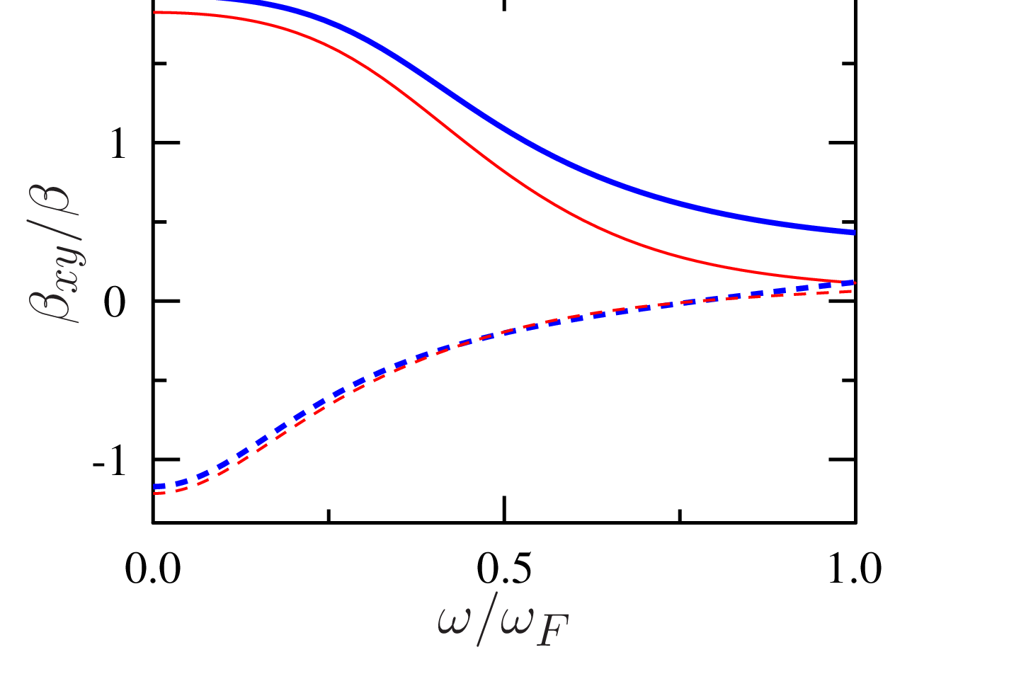
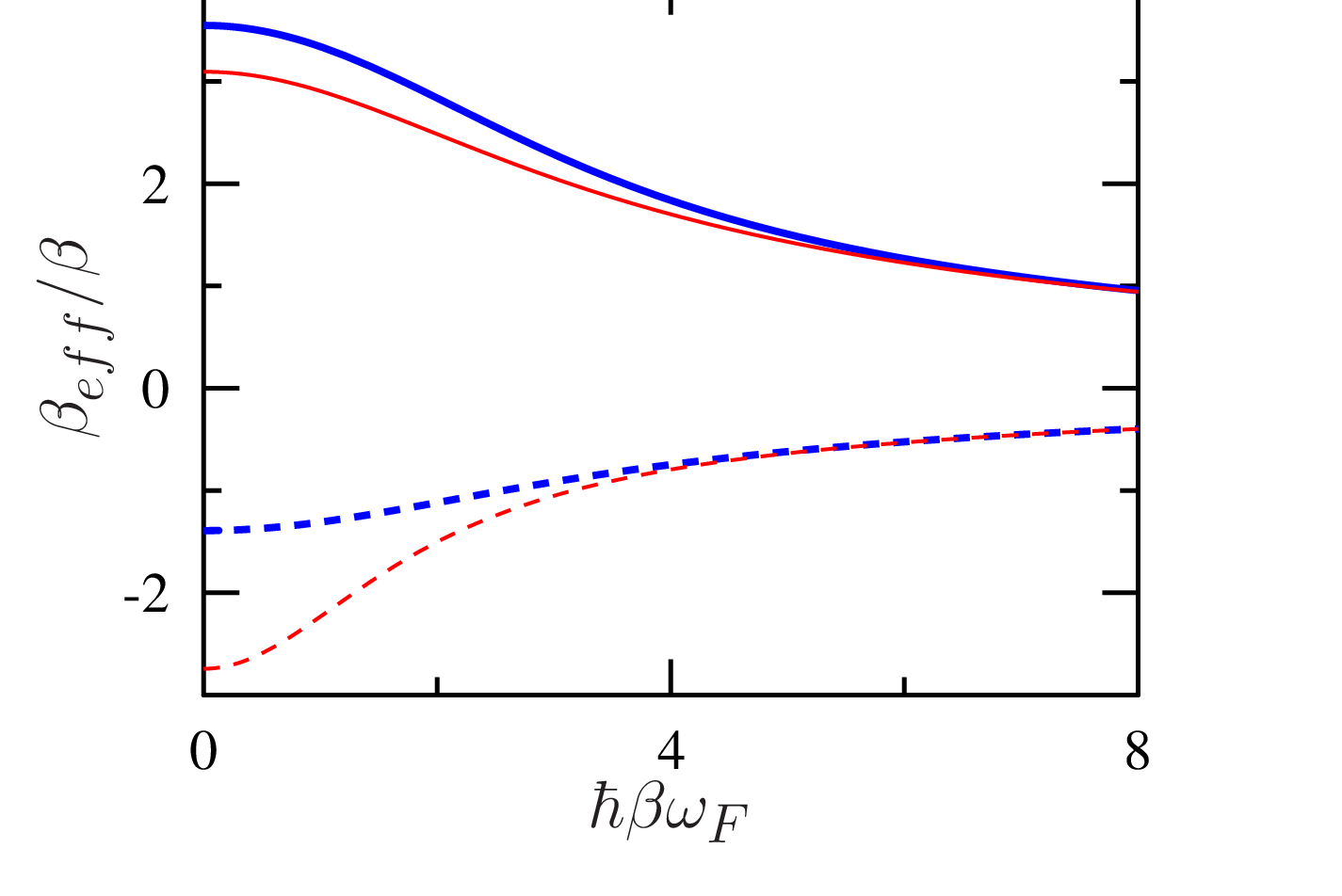
Hence, (34-35) predicts a negative effective temperature physically corresponding to the fact that absorption becomes more probable than emission and a population inversion is induced. Recent experimental observations of enhanced relaxation in a quantronium circuit coupled to a cavity bifurcation amplifier [20] may be explained qualitatively by this phenomenon. We mention in passing that the Markov approximation employed in the derivation of (15) remains valid as long as the frequency $\omega_{p}$ exceeds the typical frequency for the bare system dynamics $\Omega$.

As discussed above, the reservoir also affects the frequencies of the off-diagonal elements of the density matrix. This Lamb shift can now easily be obtained from (8) as

with the friction function

and

with

and

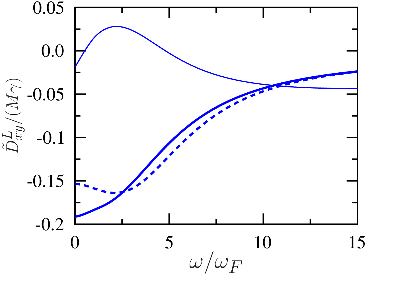
and the Matsubara frequencies $\nu_{n}=2\pi n/\hbar\beta$. Since for a purely ohmic spectral density the above expression diverges in the low as well as in the high frequency range, we take $I(\omega)=M\gamma\omega_{c}^{2}\omega^{2}/(\omega^{3}+\omega_{c}^{3})$ (see fig.5). Deviations are small in the high frequency domain, but pronounced effects occur for $\omega\approx\omega_{F}$ such that even the sign of the respective bath factors changes.

To summarize we have provided a consistent derivation of a master equation needed to capture the dissipative dynamics of periodically driven nonlinear resonators near the first bifurcation. Various expressions for the corresponding master equation have been derived and discussed. It turns out that a position-position interaction between system and bath in the laboratory frame translates into additional momentum-momentum and momentum-position couplings in the rotating frame. In case that typical transition frequencies in the rotating frame are sufficiently small compared to the external driving frequency, these latter terms are small compared to the dominant position-position coupling. The concept of an effective temperature has been introduced to analyze to what extent a detailed balance relation exists in the rotating frame. In the strict sense, one recovers detailed balance only at very low temperatures. For a structured environment phenomena such as negative effective temperatures are predicted. Explicit expressions have also been given for the Lamb-shift, which allow to better understand recent and future experimental findings.